On Partial Defaults in Portfolio Credit Risk : A Poisson Mixture Model Approach

econstor

www.econstor.eu

Der Open-Access-Publikationsserver der ZBW – Leibniz-Informationszentrum Wirtschaft

The Open Access Publication Server of the ZBW – Leibniz Information Centre for Economics

Nutzungsbedingungen:

Die ZBW räumt Ihnen als Nutzerin/Nutzer das unentgeltliche, räumlich unbeschränkte und zeitlich auf die Dauer des Schutzrechts beschränkte einfache Recht ein, das ausgewählte Werk im Rahmen der unter

→ http://www.econstor.eu/dspace/Nutzungsbedingungen nachzulesenden vollständigen Nutzungsbedingungen zu vervielfältigen, mit denen die Nutzerin/der Nutzer sich durch die erste Nutzung einverstanden erklärt.

Terms of use:

The ZBW grants you, the user, the non-exclusive right to use the selected work free of charge, territorially unrestricted and within the time limit of the term of the property rights according to the terms specified at

→ http://www.econstor.eu/dspace/Nutzungsbedingungen By the first use of the selected work the user agrees and declares to comply with these terms of use.

Weißbach, Rafael; von Lieres und Wilkau, Carsten

Working Paper

On Partial Defaults in Portfolio Credit

Risk : A Poisson Mixture Model

Approach

Technical Report / Universität Dortmund, SFB 475 Komplexitätsreduktion in Multivariaten Datenstrukturen, No. 2005,06

Provided in cooperation with:

Technische Universität Dortmund

Suggested citation: Weißbach, Rafael; von Lieres und Wilkau, Carsten (2005) : On Partial Defaults in Portfolio Credit Risk : A Poisson Mixture Model Approach, Technical Report / Universität Dortmund, SFB 475 Komplexitätsreduktion in Multivariaten Datenstrukturen, No. 2005,06, http://hdl.handle.net/10419/22597

On Partial Defaults in Portfolio Credit Risk

A Poisson Mixture Model Approach

‡

Institute of Business and Social Statistics, University of Dortmund, Dortmund, Germany

†

Central Credit Management, WestLB AG, D¨usseldorf, Germany

January 28, 2005

Abstract

Most credit portfolio models exclusively calculate the loss distribution for a portfolio of performing counterparts. Conservative default definitions cause considerable insecurity about the loss for a long time after the default. We present three approaches to account for defaulted counterparts in the cal-culation of the economic capital. Two of the approaches are based on the Poisson mixture model CreditRisk+and derive a loss distribution for an in-tegrated portfolio. The third method treats the portfolio of non-performing exposure separately. All three calculations are supplemented by formulae for contributions of the counterpart to the economic capital.

∗_{address for correspondence: Rafael Weißbach, Institute of Business and Social}

Statis-tics, Faculty of StatisStatis-tics, University of Dortmund, 44221 Dortmund, Germany, email: [email protected], Fon: +49/231/7555419, Fax: +49/231/7555284. JEL subject classifications. C51, G11, G18, G33.

1

Introduction and notation

In finance, mixture models are a common tool for modeling dependent events (see McNeil et al. (2004)). For the valuation of (single) financial products subject to credit risk, Duffie and Singleton (1999) and Lando (1998) use Bernoulli mixture models. The Bernoulli mixture model is closely related to the Poisson mixture model in the case of rare events as is the case of credit risk in commercial banking. The commercial portfolio credit risk model CreditRisk+(Credit Suisse First Boston (CSFB) (1997)) assumes a Poisson Mixture model to derive the credit loss distribution for a loan portfolio. To this end, the Poisson distribution is mixed with a Gamma distribution for the probabilities of default (PD). The methodology dates back to Green-wood and Yule (1920). For a comparison with other (commercial) models see Crouhy et al. (2000); Gordy (2000). With the help of B¨urgisser et al. (2001) we consider the latter model and mix additionally with a (Beta) dis-tribution to account for random exposures. The model allows for already defaulted exposures with still unknown losses to be incorporated into the calculation. The effect is positioned into the context of capital requirements as under discussion in Basel Commitee on Banking Supervision (2004). The calculation of the loss distribution and its variance are considered. Special emphasis is put on the fair decomposition of the economic capital (EC) into contributions for the participating engagements.

When analyzing credit portfolio risk, the loss distribution is of central interest. Theexpected loss (EL) and the economic capital(EC) are derived from it. The lossL1is the sum of all individual losses. The bank incurs a loss

of νA for the counterpartA belonging to the portfolio A when it defaults.

thus

L1=

X

A∈A

νAIA. (1)

The calculation of the distribution of L1 has been under investigation for

a long time in insurance mathematics (see e.g. Klugman et al. (1998)). In order to account for (stochastic) dependencies between defaults of different counterparts, the approach in CreditRisk+is to assume randomprobabilities of default(PD). We use the established model

µA=pA

K

X

k=1

θA,kXk, (2)

whereθA,k denotes the weight of counterpart A with respect to the factors Xk, k = 1, . . . , K. The latter are often taken to be industry branches or

countries. We assume as usual that the defaultsIA are independent,

condi-tional on X = (X1, . . . , XK). An obvious assumption is that PKk=1θA,k =

1 ∀ A ∈ A. The Xk’s are assumed to be Γ(σk−2, σ2k) distributed, and thus E(Xk) = 1, E(IA) = pA and V ar(Xk) = σ_k2. In the version of Credit

Suisse First Boston (CSFB) (1997) the Xk’s are assumed to be

indepen-dent. However, B¨urgisser et al. (1999) allows for dependent sector vari-ables to be used which we will make use of in the end with covariances

ckl=Cov(Xk, Xl), k, l= 1, . . . , K.

From a banking perspective, the assumption of the randomness in the individual loss νA is even more realistic. The loss given default (LGD)

identifies the portion of the exposure at default (EAD) of a counterpartA, which can not be regained in case of a default. The CreditRisk+ _model

assumes that the net exposureνA=eAlA, where eAdenotes the EAD and

lA the LGD of a counterpart A, is known. However, one observation in

the diversification would suggest that the overall effect is negligible. In fact, to assume the independence of LGD’s across counterparts is implausible. Empirical evidence from time series exists proving the converse. This is also intuitive. Often, the LGD depends on collateral, which may be any asset. The value of an asset is surely related to the general economic activity leading to dependent values of collateral and dependent magnitudes of the LGD. For a similar approach see Grundke (2004). We need to account for a stochastic LGD in the calculation of the portfolio loss distribution. Recently, B¨urgisser et al. (2001) proposed a means to integrate a stochastic LGD under certain distributional assumptions into the loss distribution. We will briefly review the method in Section 2.

In the case of the stochastic PD the notion is that the economic activ-ity (at the beginning of a year) takes shape, and the counterparts default consecutively (within the year) according to their PD’s. For the defaulted exposure, the cascade goes even further down. If the counterpart defaults, the LGD is still random. Only after the settlement of the claims (e.g. to the default agent) will the realized loss be known. The definition of bankruptcy in banking is conservative in order to put an early incentive towards inten-sive treatment of endangered engagement. A bank might well be exposed to a counterpart years after default occurs. The creditor needs to integrate the insecurity about the unknown risk into his loss forecast. Allowing for mul-tiple defaults is not feasible because the PD is usually only available for the first default. However, for the calculation of the portfolio loss distribution, we may account for insecurity in terms of the LGD parameter. B¨urgisser et al. (2001) allows for the treatment of the latter case.

Let in the followingλAdenote the stochastic LGD with the expectation E(λA) =lA. Clearly, the expected loss of the portfolio is not changed if the

PD’s are independent of the LGD’sλA. EL1(λA, A∈ A) = X A pAeAE(λA) = X A pAeAlA=EL(lA, A∈ A), pA denotes the expected PD of counterpartA.

The paper is organized as follows. In Section 2 the one-factor model of B¨urgisser et al. (2001) is applied to incorporate defaulted exposure. Section 3 uses more factors to allow for imperfect correlation between the LGD’s of segmented counterparts. Both approaches make use of the CreditRisk+

algorithm and allow for risk to be diversified across the entire portfolio. Per-forming and non-perPer-forming portfolios are treated simultaneously. Section 4 is devoted to the necessity of calibrating the two models. Section 5 separates the portfolios and enables a calculation of risk contributions for defaulted counterparts without affecting the performing portfolio. A latent one-factor model is fitted to historical data.

2

One-factor model

Consider the following simple model for the loss given default (LGD) (cf. B¨urgisser et al. (2001)):

λA=lAΛ, (3)

where Λ is a random variable with expectation 1 and variance δ2, which is independent of the defaults IA, A ∈ A. The portfolio loss can now be

written as ˜ L1:= X A eAlAΛIA= Λ X A eAlAIA= ΛL1. (4)

Clearly, the expected lossE( ˜L1) is again equal toE(L1).

The loss distribution can be calculated as ˜ F1(k) := P( ˜L1 ≤k) =P(Λ≤k/L1), k/0 :=∞ = X n≥0 P(Λ≤k/L1 |L1 =n)P(L1 =n) = P(L1 = 0) + X n≥1 P(Λ≤k/n)P(L1 =n) = f_LCR+ 1 (0) + X n≥1 f_LCR+ 1 (n)FΛ(k/n), (5) withf_LCR₁ +(n) :=P(L1 =n) andFΛ(n) :=P(Λ≤n), n= 0,1, . . ..

The notation for the distribution ofL1 stresses that it can be calculated

using the algorithms CreditRisk+ (see Credit Suisse First Boston (CSFB) (1997)). Sometimes, we will use f_LCR₁ +(eAlA, pA, σ_k2, θA,k A ∈ A, k =

1, . . . , K), i.e. attach all parameters.

Based on the work of B¨urgisser et al. (2001) we would like to devote ourselves to the following issue of practical importance. The default of a counterpart is economically fixed to the date of the first default on an allying payment. At that point in time, we can model the default as a Bernoulli experiment with parameter 1. It is common in financial institutions to make provisions on the event of default. In the model with deterministic LGD’s no further insecurity is left, and thus the counterpart must be excluded from the calculation of the loss distribution. However, the definition of default implies that the magnitude of final loss is not yet known. The case of a stochastic LGD applies. The risk is that the final overall loss will be greater than the provision.

The definition (4) of the portfolio loss needs a generalization which we provide in the following

Definition 2.1 ˜ L:= X A /∈E eAλAIA+ X A∈E eAλA= ˜L1+ ˜L2

where L˜1 := PA /∈EeAλA IA is the loss from the so-called performing

port-folio and L˜2 := PA∈EeAλA is the loss from the non-performing portfolio.

The set E denotes the defaulted counterparts. We will sometimes refer to the performing portfolio with the notation Ec_.

Owing to the model (3) (λA = lAΛ) we can decompose L˜1 and L˜2 into

˜

L1= ΛL1 and L˜2 = ΛL2 with L1 :=PA /∈EeAlAIA and L2 :=PA∈EeAlA,

respectively.

For the ease of notation let L˜ := ΛL with L:=L1+L2.

Note that the definitions ˜L1 and L1 fit the definitions in the model

without defaulted counterparts (see (4)). ˜L2 constitutes the (random) loss

arising from the sub portfolio of defaulted counterparts. To stress that L2

is deterministic we will denote it byη in the sequel.

The calculation of the loss distribution is analogous to the distribution of ˜L above

˜

F(k) =P( ˜L≤k) =fL(0) +X

n≥1

fL(n)FΛ(k/n), (6)

where nowfL(·) is only dependent on fL1(·),

fL(n) =P(L=n) =P(L1=n−η) =fL1(n−η). (7)

fL(0) can only be positive ifE =∅; we will not consider this degenerate case. fL1 can be calculated with the Panjer recursion (see Panjer and Willmot

(1992)) as proposed in Credit Suisse First Boston (CSFB) (1997). For an alternative proposal see Giese (2003).

As a first result we now have a procedure for calculating any high quantile of the loss distribution known as credit value-at-risk CreditV aR.

Theorem 2.1 Let the loss L1 for a portfolio of not defaulted counterparts

with deterministic LGD’s according to Definition 2.1 be distributed according to f_LCR₁ +(eAlA, pA, σ2k, θA,k A ∈A, k = 1, . . . , K). Then in a portfolio with

LGD’s according to model (3), factor Λ with cdf Fλ(·) and an additional

portfolioE of defaulted counterparts with expected exposureη=P

A∈EeAlA

the credit value-at-risk at level γ is given by

CreditV aRγ = inf    k:X n≥1 f_LCR₁ +(n−η)FΛ(k/n)> γ    .

The economic capital (EC) is defined as the difference between the credit value-at-risk at level γ and the expected loss.

Corollary 2.1 Under the assumptions of Theorem 2.1 the economic capital for a joint portfolio of not defaulted and defaulted counterparts is given by

ECγ =CreditV aRγ− X A /∈E pAeAlA+ X A∈E eAlA ! .

Corollary 2.1 follows from E( ˜L) =E(Λ)(E(L1) +η) =PA /∈EpAeAlA+

P

A∈EeAlA.

For the next step we need the loss variance

V ar( ˜L) = E(V ar( ˜L1+ ˜L2|Λ)) +V ar(E( ˜L|Λ))

= E(Λ2V ar(L1+η)) +V ar(ΛE(L))

= E(Λ2)V ar(L1) +E(L)2V ar(Λ)

An important issue in portfolio risk is the attribution of the risk to the responsible counterparts. As standard procedure, Credit Suisse First Boston (CSFB) (1997) propose to consider the portfolio loss varianceV ar( ˜L) a risk measure and attribute the risk according to the change in variance as the exposure νA changes. An additive risk attribution is guaranteed for the

definition ˜ vcA:= eA 2 ∂σ˜2 ∂eA = eA 2 (1 +δ2) ∂σ 2 1 ∂eA +δ2 ∂(ε+η) 2 ∂eA , with notationσ2 1 :=V ar(L1), σ˜2 :=V ar( ˜L), ε:=E(L1).

With the notation of the PD model (2), a lengthy calculation yields

σ2₁ =X A /∈E e2_Al_A2 pA  1−p_A  1 + K X k,l=1 cklθA,kθA,l    + K X k,l=1 cklεkεl, (9)

where the expected loss in sectorkis denoted by

εk=

X

A /∈E

θA,kpAeAlA. (10)

The variance contribution is now twofold, according to whether counter-partA defaulted or not.

Theorem 2.2 For the loss modeled in Definition 2.1 of a credit portfolio with performing and defaulted exposures, additive variance contributions are given by ˜ vcA=pAeAlA pAeAlA˜cA+ ˜dA . (11) HeredA,k:=PK

l=1cklεl,−A andεl,−A:=P_{B /}∈E∪AθB,l pBeBlB.Additionally, pA= 1 for counterparts A∈ E and the notation

˜

cA= (1−pA+δ2)/pA, d˜A= (1 +δ2)PKk=1θA,kdA,k+δ2(ε−A+η) A /∈ E

˜

where ε−A=PB /∈E∪ApBeBlB and η−A=PB∈E,B6=ApBeBlB

IfA /∈ E we have ˜vcA=pAeAlA((1+δ2)(eAlA(1−pA)+PKk=1θA,kdA,k)+

(ε+η)δ2_{), whereas forA∈ E we have ˜vc}

A=eAlA(ε+η)δ2.

The representation (11) is similar to the original variance contribution in Credit Suisse First Boston (CSFB) (1997). The key conclusion that can be drawn from the representation is the penalty for large single exposures

eA, which is reflected by the quadratic component.

However, the contribution to the variance is only an intermediate step. A key question in finance is the allocation of economic capital for pricing, costing and budgeting. We need a portion of the EC attributable to each counterpart so that the contributions add up to the EC and the cause-effect model holds. We do already have a notion of cause and cause-effect for the dependence of the loss variance on the exposure of each counterpart. The EC and the loss variance are closely related. Both are measures for the potential deviation of the loss from its expectation. We will now assume that the EC exhibits the same sensitivity with respect to the exposure of each counterpart as the variance does.

The number ecA= PvcA˜ Bvc˜B ECγ= vcA˜ ˜ σ2 ECγ (12)

constitutes an approximate contribution of the exposure of counterpart

Ato the EC obeying P

AecA=ECγ.

Note that we allow for correlation between the sector variables Xk in the calculation of the loss variance (9). However, the calculation of the

CreditV aRγ in (12) is achieved from Theorem 2.1, where the sectors are

of B¨urgisser et al. (1999) to incorporate the correlation into the calculation of the credit Value-at-Risk.

Remark 1. An alternative to establishing a cause-effect attribution of the EC to each counterpart consists in calculating the EC with the whole portfolio and separately with the portfolio leaving out one counterpart. The difference between the two values can be interpreted as the risk contribution of the counterpart. However, the approach has two disadvantages. On the one hand, the attribution is not additive, and the sum of all contributions thus derived is usually less than the EC. The “late coming counterpart” profits from the existing diversification. The procedure could be refined by using an idea from game theory. One could add the counterparts subse-quently to the portfolio and average over all possible sequences. This leads us to the second drawback. The computational effort for large portfolios is sizeable even for the leave-one-out approach (of orderN, the number of counterparts in A). For the complete enumeration the factor is of order

PN

i=1 Ni

, e.g. 1030_{forN = 100.}

Remark 2. The incorporation of the defaulted counterparts into the total loss calculation affects the risk contributions for counterparts not in default. The changes are noticeable, and thus one preliminary aim may be to calculate risk contributions for defaulted counterparts independently of the performing portfolio. To this end, we need to calculate the economic capital for the portfolio without the defaulted counterparts and derive risk contribution of that. In a second stage we need to calculate the distribution (and EC) for the entire portfolio to determine the increase in EC caused by the non-performing portfolio.

described procedure, we define forA /∈ E ecA:= ˜ vc(1)_A P B /∈Evc˜ (1) B EC_γ(1) (13)

whereECγ(1):=CreditV aR(1)γ −E( ˜L1) andCreditV aR(1)γ = inf{k:P( ˜L1 ≤

k)> γ} denotes the Value-at-Risk. The variance contributions for the not defaulted exposures are denoted by ˜vcA, A /∈ E. Note for ˜σ12 =V ar( ˜L1):

˜ vc(1)_A := eA 2 ∂σ˜2₁ ∂eA = eA 2 (1 +δ2) ∂σ 2 1 ∂eA +δ2 ∂ε 2 ∂eA = pAeAlA (1 +δ2)eAlA(1−pA) + K X k=1 θA,kdA,k +εδ2.

The ecA is now calculated as in (13). For A∈ E the marginal contribution

of the non performing portfolioECγ−ECγ(1) can be distributed according

to the expected individual loss. Finally, the expected individual loss is subtracted ecA:= eAlA P B∈EeBlB (ECγ−ECγ(1)) (14)

to obtain again the necessary requirement P

AecA=ECγ.

3

Multi-factor model

The one-factor model (3) in Section 2 assumes that the LGD’s of the coun-terparts are perfectly correlated. We will now relieve the assumption of one latent LGD factor Λ and allow for inhomogeneous LGD correlations. The LGD of a counterpart is assumed to follow the model

λA=lAΛA M

X

j=1

wA,j Λj (15)

A1 The random variables Λj, j= 1, . . . , M are independent of the defaults IA, A= 1, . . . , N withE(Λj) = 1 and V ar(Λj) =δj2.

A2 The ΛA, A= 1, . . . , N, are independent of the Λj, j= 1, . . . , M,and

theIA, A= 1, . . . , N, withE(ΛA) = 1 andV ar(ΛA) =δ2A.

A3 For all Aholds wA,j ≥0, j= 1, . . . , M,and PMj=1wA,j = 1.

Before the calculation of the portfolio loss distribution, we will first con-sider its variance

˜ σ2 = X A /∈E e2_Al2_ApA(1 +δ_A2)−pA(1 + K X k,l=1 cklθA,kθA,l)1 + M X i,j=1 aij wA,iwA,j + M X i,j=1 K X k,l=1 aij cklε(ki)ε (j) l + K X k,l=1 cklεkεl + M X i,j=1 aij ε(i)ε(j)+ 2ε(i)η(j)+η(i)η(j) + X A∈E e2_Al2_Aδ2_A1 + M X i,j=1 aij wA,iwA,j , (16)

whereaij :=Cov(Λi,Λj), εk as in equation (10), ε(_ki)=X A /∈E θA,kwA,i pAeAlA, ε(i)= X A /∈E wA,ipAeAlA and η(i)=X A∈E wA,ieAlA. (17)

For the calculation of the loss distribution we follow the old statistical idea of moment fitting (which B¨urgisser et al. (1999) used to integrate cor-relations for the economic activity variables Xk into the loss distribution).

As the expectation is not changed by random LGD’s at all, we fit the vari-ance of the loss for the LGD multi-factor model (15) to the varivari-ance of a

one-factor model (3). We approximate the distribution of the multi-factor model by the distribution of the one-factor model. The reason for the sim-plification is technical, since the loss distribution would otherwise no longer be given in closed form. A numerical evaluation, i.e. a numerical integra-tion, would constitute a second numerical procedure, because the derivation of the loss probabilities from the probability generating function must also be established using numerical differentiation (with the Panjer recurssion).

Theorem 3.1 Let the loss L1 for a portfolio of not defaulted counterparts

with deterministic LGD’s according to Definition 2.1 be distributed according to f_LCR₁ +(eAlA, pA, σ2_k, θA,k A ∈A, k = 1, . . . , K). Then in a portfolio with

LGD’s according to model (15) fulfilling assumptions A1-3 and an additional portfolioE of defaulted counterparts with expected exposureη=P

A∈EeAlA.

If it holds true that the loss distribution for the multi-factor model is equal to the distribution for the one-factor model (3) if the first two moments are equal, then the credit value-at-risk at level γ is given by

CreditV aRγ = inf    k:X n≥1 f_LCR₁ +(n−η)FΛ(k/n)> γ   

whenever the volatilityδ2 _{of the (equivalent) factor Λ is given by}

δ= s ˜ σ2_−v 1−v2 v1+v2+ (ε+η)2 , withv1=PA /∈Ee2Al2ApA 1−pA(1+PKk,l=1cklθA,kθA,l) andv2=PKk,l=1cklεkεl.

Proof: For the caseM = 1 andδA= 0 holds for all A (see (8) and (9))

˜ σ_M2 _{=1, δ} A=0 = (1 +δ 2_)(v 1+v2) +δ2(ε+η)2 = v1+v2+δ2(v1+v2+ (ε+η)2).

In order to obtain the variance of the factor Λ in the equivalent one-factor model we set ˜σ2 _{= ˜σ}2

M=1, δA=0.

The calculation of the EC follows Corollary 2.1.

We have now enabled the calculation of the economic capital, as in the one-factor model in Section 2.

In order to derive risk contributions, we follow the same line as in Section 2. The variance contributions in the multi-factor model (15) only depend on the loss variance which is - in contrast to the loss distribution - exactly given.

Theorem 3.2 Consider the loss modeled in Definition 2.1 of a credit port-folio with performing and defaulted exposures. The LGD λA is assumed to follow (15). Then, additive variance contributions are for A /∈ E given by

˜ vcA = e2Al2ApA (1 +δ_A2)−pA(1 + K X k,l=1 ckl θA,kθA,l) 1 + M X i,j=1 aij wA,iwA,j + eAlApA XM i,j=1 aij wA,i(ε(j)+η(j)+ K X k,l=1 θA,kε(_lj)) + K X k,l=1 cklθA,kεl (18) For A∈ E holds ˜ vcA=e2AlA2δA2 1+ M X i,j=1 aijwA,iwA,j +eAlA M X i,j=1 aijwA,i ε(j)+η(j). (19) The contribution to economic capital can now again (see 12) be defined asecA:= _Pvc˜A

Bvc˜B ECγ.

Remark 2 - continued. In the last section we considered the problem of dependence between the non-performing portfolio E and the performing portfolio (Ec). One might strive for an uncoupled calculation of economic capital charges in the two portfolios for the LGD multi-factor model as well.

The performing portfolio is treated as “stand alone”. The EC for the non-performing portfolio is taken to be an increase in the EC when it is added to the performing portfolio, i.e. taken as ECγ −ECγ(1). The latter

eco-nomic capital for the defaulted counterparts may be attributed to the single counterpart in proportion to the expected loss as in the single factor model (see (14)). However, the variance contribution for the performing portfolio needs further attention. The formula (18) describes a contribution in the case of the LGD multi-factor model when the variance of the whole portfo-lio is decomposed. However, the simplification in the absence of defaulted exposure is minimal. Only the termsη(j) _{must be omitted, which represent}

the expected loss in the LGD class j for the defaulted exposure.

4

Calibration of the models and impact study

We restrict ourselves to the calibration of the one-factor model described in Section 2. The multi-factor model from Section 3 may be calibrated accordingly in the presence of data stratified to LGD classes.

A common distributional assumption for the factor Λ as defined in (3) is the log-normal distribution (see B¨urgisser et al. (2001)). However, the LGD is bounded at both sides because the loss after settlement of all claims ranges between 0% and 100% of the exposure at default. And, empirically, the log-normality does not fit very well. Assuming a uniform distribution, we found that the boundaries of the uniform density are more pronounced than the empirical ones in our sample. A generalization is the Beta distribution (as we will clarify below). The use of the Beta distribution for the recovery rates (which is the inverse of the LGD) is propagated in Grundke (2004). Based on data of a cooperating bank we found that the Beta distribution fits for

the distribution of Λ with some modifications. Now we discuss the use of the distribution and add empirical evidence, once the parameter estimates are presented.

As distribution for the factor Λ we assume an affine transformation of the Beta distribution, i.e.

Λ∼a+ (b−a)Beta(α, β), (20)

where 0≤a <1< bandα, β >0. Beta(α, β) denotes the Beta distribution with parametersαandβand densityxα−1_(1−x)β−1_{/B(α, β) withB(α, β) =}

Γ(α)Γ(β)/Γ(α+β) and Γ(α) =R∞

0 exp(−x)xα−1dx.

The assumption 1 = E(Λ) = a+ (b−a) α/(α+β) forces β = α (b−

1)/(1−a). The parameterβ is fixed given a, band α.

For the variance,V ar(Λ) = (b−a)2_{αβ/((α+β)}2_{(α+β+ 1)) holds.}

A special case isb−1 = 1−aand α=β = 1, where the distribution is uniform around 1 on the symmetric interval [a,2−a].

Remark 3. In order to accelerate the computation of the value-at-risk arising from Theorem 2.1, we restrict the definition of the Beta distribution to the discrete points 10−5_{×N, i.e. F}

Beta(α,β) is replaced by ˆ F_Beta(α,β)= n−1 X i=0

F_Beta(α,β)(i/n)I_{[i/n,(i+1)/n)} (n= 10000).

Thus, the processing time is drastically reduced.

Remark 4. Additionally, the distribution function of ˜L need not be calculated entirely. The new value-at-risk is obtained by nested intervals, which again reduce the computation markedly. Obviously, the value-at-risk increases due to the additional variability of exposure and increased business coverage. Hence, the iteration starts at the value-at-risk for the performing portfolio without stochastic LGD, i.e. at theγ-quantile off_LCR₁ +(·).

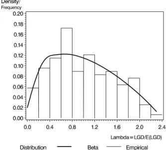
Table 1: Elementary statistics of the empirical relative LGD

Mean Std Min Max

Empirical 1 0.5686 0.0512 2.5817

Beta 1 0.56 0.05 2.4

As mentioned in the beginning, the calibration of the model is performed with historical data. The descriptive statistics are given in Table 1. A model fit is derived heuristically using Figure 1. The parameters a = 0.05, b = 2.4, α= 1.31, β= 1.93 lead to sensible results.

Figure 1: Distribution of Λ in comparison to the empirical relative LGD movement

We can now assess the impact of the developed enhancement. To this end, we need a benchmark. A simple (and typical) treatment of defaulted

exposure is to add their expected loss to the expected loss of the performing portfolio. The loss distribution of the performing portfolio is simply shifted to the right. The loss distribution for the performing portfolio is calculated neglecting the stochastic LGD by using expected LGD’s and treating them as deterministic (and known in advance).

Let us first determine the effect of incorporation of the LGD stochastic. We compare the latter approach to our method based on the one-factor model (3) in the Definition 2.1 for the loss and with value-at-risk according to Theorem 2.1. The performing portfolio we study is realistic – although fictitious – for an international bank. It consists of around 5000 exposures distributed asymmetrically over 20 sectors (denoted byXkin definition (2))

with 20 to 500 counterparts per sector. The total exposure is 35 billion Euro with the largest exposure of 0.7 billion Euro and the smallest exposure of 0.1 million Euro. The counterpart specific default probability varies between 0.03% and 7%. By using the parameters mentioned above we find that the one-factor model suggests a value-at-risk which is 1.55 times higher than the value-at-risk with the deterministic approach.

Clearly, if we add a non-performing part, the increase in value-at-risk is even higher. The shift to the right in the simplified approach ignores the variability of the LGD in the non-performing portfolio and hence the credit value-at-risk is underestimated. The quantification crucially depends on the portion of non-performers in a the whole portfolio. But the latter is governed by the business area and policy of work-out treatment on defaulted counterparts differing across banks. A quick settlement of claims can reduce the portion whereas e.g. long negotiations will increase the portion. We cannot think of a typical case, and thus we must refrain from a quantification here. However, a heuristic reason why the effect must be substantial goes as

follows. The ratio of value-at-risks in the performing portfolio of 1.55 is only due to the LGD stochastic. The variability arising from the random PD’s and the Bernoulli events as such are already accounted for in both models. Diversification between the LGD and the other two stochastic effects reduces the effect of each single source. For the non-performing portfolio, the LGD stochastic is the only source of insecurity. The increase in value-at-risk of the non-performing portfolio in the simplified method is the expected loss. The increase in value-at-risk in our method is implicitly given as the difference of the value-at-risk of ˜Lan ˜L1. Clearly, the increase in terms of ratio between

expected loss from the non-performing portfolio and the marginal value-at-risk using our method is larger than 1.55.

5

Further Remarks and Extensions

Along the lines of Remark 2 in Section 2, we now consider the task of estab-lishing an independent calculation of the loss distribution for the portfolio of defaulted counterparts whose exposure is not yet completely provisioned. The portfolio in mind may be under a separate response and management, and thus an independent assessment may be needed. Or, it is simply not plausible that defaulted counterparts have an impact on the performing portfolio. To lay out the methodological details, we denote withνA the

ex-posure at default (EAD) of the defaulted counterparts A∈ E. The change of provision for counterpartAin yeartis denoted ∆At, whereas the relative

change of the provision with respect to the first date of provision (which is the date of default) is δAt (δAt= ∆At/νA).

factorYt which models economic activity:

δAt=Yt+At A∈ E, t= 1, . . . , T. (21)

The idiosyncratic variability of the relative provision for counterpart A

in yeart is represented by the noiseAt.

We assume the Yt’s and the At’s to be independently normally

dis-tributed (N(µ, σ2

Y) and N(0, σ2), respectively), i.e. we assume the absence

of higher cumulants because the amount of data does not allow us to prove those effects. The distribution is assumed to be the same for all points in timet. The common correlation ρ determines the relation of the variances of Yt and At. For A6= ˜A, ρ =corr(δAt, δ_At˜) = σY2/(σ2Y +σ2) holds, which

is equivalent to σ_Y2 = ρσ2/(1−ρ). For the variance σ2_δ of the normally distributed variableδAt follows

σ_δ2=σ2_Y +σ2=σ2/(1−ρ). (22)

We see that σ_δ2 is determined by the variance σ2 of the At’s and the

correlation ρ. We will explore the connection while estimating the variance

σ_δ2.

We estimate the pairwise correlation between δAt and δ_At˜ with

ˆ ρ_AA˜:= T X t=1 (δAt−δ¯A·)(δ_At˜ −δ¯_A˜·)/ v u u t T X t=1 (δAt−δ¯A·)2 T X t=1 (δ_At˜ −¯δ_A˜·)2,

where ¯δA· denotes the mean of the δAt’s with respect to time t, ¯δA· :=

PT

t=1δAt/T. The common correlation is estimated as

ˆ ρ:= 2X A∈E X ˜ A∈E ˆ ρ_AA˜/(]E(]E −1)), (23)

The individual noises At are not observable. However, their variance σ2

can be estimated from the observable δAt’s ˆσ2 :=

PT t=1 P A∈E(At − ¯ ·t)2/(]ET) =PTt=1 P

A∈E(δAt−δ¯·t)2/(]ET), where ¯·t:=PA∈EAt/]E and

¯

δ·t:=P_A˜∈EδAt/]E =

P

˜

A∈E(At+Yt)/]E=·t+Yt.

The variance σ_Y2 of the latent economic activity Yt is estimated using

formula (22) as ˆσ2

Y := ˆσ2ρ/ˆ (1−ρˆ) as well as formula (22) enables us to

estimate the variance of theδAt’s as

ˆ

σ_δ2:= ˆσ_Y2 + ˆσ2 = ˆσ2/(1−ρˆ) (24)

The last parameter we want to estimate in our one-factorial model (21) is the location,µ=E(Yt) =E(δAt) ˆ µ:= T X t=1 X A∈E δAt/(]ET) (25)

We now have sufficient information to calculate the credit value-at-risk of the non-performing portfolio.

The loss generated by the portfolio at time tis

Zt= X A∈E ∆At= X A∈E νAδAt.

The loss Zt is independent of t, i.e. stationary, and Zt∼N(µ, σ2Z) with σ_Z2 =   X A∈E ν_A2 + X A,A˜∈E,A6= ˜A νAν_A˜ρ  σ2_δ (26)

The current state of provisions for the already defaulted counterparts reflects the expected amount of the loss arising from the non-performing portfolio. The variable Zt defines the unexpected loss of that portfolio for

Table 2: Values ofuγ for a typicalγ γ uγ 99.95% 3.29 99.50% 2.58 99.00% 2.33 90.00% 1.28 75.00% 0.68

economic capital) from the normal distribution of Zt. With probability γ

the variableZt will express below

Zγ=µ+uγσZ, (27)

whereuγ denotes theγ-quantile of the standard normal distribution.

Typical values for uγ are given in Table 2.

The distribution of Zt is asymptotically unchanged if the parameters µ and σ2_Z are estimated consistently, as is the case for the estimate (25) for µ and the canonical estimate derived from (23) and (24) for σ2

Z in its

representation (26). The reason is Slutsky’s theorem, see e.g. Ferguson (1996)).

Again, the calculation of the economic capital for the non-performing portfolio is derived by subtracting the expected lossµ(or rather its estimate) from the credit value-at-risk (27).

The risk contributions for the separate exposures can now be attributed, e.g. proportionally with respect to the exposure

˜ rcA:=νA  µˆ+u_γσ_δ s X A∈E ν2 A+ X A,A˜∈E,A6= ˜A νAν_A˜ρ  / X A∈E νA. (28)

An alternative is to attribute the economic capital proportional to the ex-pected loss (given default) which did change the denominator toP

A∈ElAνA

and the νAat the beginning of the numerator to lAνA.

Remark 5. We find it important to note that even the simple approach described above incorporates diversification. We may see the risk contri-bution (28) as percentage of νA (timesνA). The factor ˜rcA/νA is of order O(]E−1/2_{) if the correlationρis 0. This can be seen by usingν}

A= 1

through-out. The risk vanishes for an infinitely large portfolio. If the correlation is perfect, i.e. ρ= 1, the order isO(1), no diversification due to portfolio size is possible.

6

Conclusion

We have proposed three methods to calculate risk contributions for non-performing exposure in portfolio credit risk. The economic risk is calculated together with the performing portfolio and separately. The main suggestion is to use a Poisson mixture model, equivalent to CreditRisk+_{, and}

incor-porate a (Beta) mixture distribution for the loss given default (LGD). In the latter setup a one-factorial design of the LGD is described in detail. A multi-factorial generation of the LGD is included allowing for more realistic situations. These two approaches imply dependencies between the perform-ing portfolio and the non-performperform-ing portfolio. The dependency can be relieved for the calculation of the risk contributions only. To this end, one may use the marginal contribution of the non-performing portfolio for the overall economic capital and distribute it across the originators. Or, if a full disconnection between the two portfolios is wanted, we propose a simple stand-alone method. The LGD is modeled with a normal (Merton-type)

one-factor model and the economic capital is derived and contributions for the counterparts defined. Our theoretical calculations are supplemented by calibration of the LGD models based on real historical data and an exem-plary impact study.

Acknowledgement: We would like to thank Trudy Houghton for useful discussions and acknowledge the financial support of DFG, SFB 475 “Re-duction of Complexity in Multivariate Structures”, project B1. The views expressed here are those of the authors and do not necessarily reflect the opinion of WestLB AG.

References

Basel Commitee on Banking Supervision (June 2004). International con-vergence of capital measurement and capital standards. Technical report, Bank for International Settlements.

B¨urgisser, P., Kurth, A., and Wagner, A. (2001). Incoporating severity variations into credit risk. Journal of Risk, 3(4):5–31.

B¨urgisser, P., Kurth, A., Wagner, A., and Wolf, M. (1999). Integrating correlations. Journal of Risk, 07:57–60.

Credit Suisse First Boston (CSFB) (1997). CreditRisk+: A credit risk man-agement framework. Technical report, Credit Suisse First Boston. Crouhy, M., Galai, D., and Mark, R. (2000). Comparative analysis of current

credit risk models. Journal of Banking and Finance, pages 59–117. Duffie, D. and Singleton, K. (1999). Modeling term structures of defaultable

Ferguson, T. (1996). A course in Large Sample Theory. Chapmann & Hall, London.

Giese, G. (2003). Enhancing CreditRisk+. Journal of Risk, 16:73–77. Gordy, M. (2000). A comparative anatomy of credit risk models. Journal

of Banking and Finance, 24:119–149.

Greenwood, M. and Yule, G. (1920). An inquiry into the nature of fre-quency distributions representative of multiple happenings with particu-lar reference to the occurence of multiple attacks of disease or of repeated accidents. Journal of the Royal Statistical Society, 83:255–279.

Grundke, P. (2004). How important is the modeling of interest rate and credit spread risk in standard and non-standard credit portfolio models? Technical report, University of Cologne.

Klugman, S., Panjer, H., and Willmot, G. (1998). Loss Models: From Data to Decisions. John Wiley & Sons Inc., New York.

Lando, D. (1998). Cox processes and credit risky securities. Review of Derivatives Research, 2:99–120.

McNeil, A., Frey, R., and Embrechts, P. (2004). Quantitative Risk Man-agement: Concepts, Techniques and Tools. www.math.ethz.ch/ mc-neil/book.html.

Panjer, H. and Willmot, G. (1992). Insurance risk models. Society of actu-aries, Schaumberg, IL.