VARIABLE SCREENING AND MODEL SELECTION IN CENSORED QUANTILE REGRESSION VIA SPARSE PENALTIES AND STEPWISE REFINEMENT
BY LU GAN
DISSERTATION
Submitted in partial fulfillment of the requirements for the degree of Doctor of Philosophy in Statistics
in the Graduate College of the
University of Illinois at Urbana-Champaign, 2014
Urbana, Illinois
Doctoral Committee:
Professor Douglas Simpson, Chair Professor Stephen Portnoy, Co-Chair Professor Roger Koenker
Abstract
Many variable selection methods are available for linear regression but very little has been developed for quantile regression, especially for the censored problems. This study will look at the possibilities of utilizing some existing penalty variable selection methods on censored quantile regression problems.
In the situation when censored values are not known for each observation, it is common to model the censoring as random. Under the assumption that 𝑦! and 𝐶! are conditionally independent given 𝑥!, we use the random censored quantile regression Portnoy estimators (2010). This method simplifies the censored problem into a weight problem. When combined with the penalized regression method: LASSO and SCAD, one can perform variable screening for the censored data at quantiles of interest. Furthermore, we establish the asymptotic property, and illustrate the methodology in the context of ultrasound safety study.
Acknowledgement
First and foremost, I would like to express my ultimate gratitude towards my beloved advisor Prof. Simpson and co-advisor Prof. Portnoy, for their unbreakable patience and endless support and the wealth of knowledge they have provided. Without them I wouldn’t be able to achieve what I have today.
I would like to thank Prof. Liang and Prof. Koenker for their insightful feedback, which helped me improve my dissertation in many ways.
I would like to thank the rest of the faculty and staff members in the Department of Statistics at the University of Illinois for their assistance throughout my graduate study.
Special thanks goes to my husband Wei and my dearest son Dylon, for the endless joy and love you have given me.
Finally, I want to thank my father for his love and wisdom. Although I will not find you in the crowd when I stand on that stage, but you will always be with me in my heart. I miss you dad.
Table of Contents
List of Tables ...vii
List of Figures ...viii
List of Abbreviations ...ix
Chapter 1 Introduction ...1
1.1 Censored Regression Quantile ...1
1.2 Penalized Variable Selection Methods ...5
Chapter 2 Penalized Quantile Regression for Variable Selection ...7
Chapter 3 Large Sample Theory for Censored Penalized Quantile Regression ...13
Chapter 4 Case Study ...25
4.1 Penalized Model Screening - LASSO ...28
4.2 Extension of Portnoy Estimator – Inference Based Refinement of Screened Variables ...33
4.3 Penalized Model Screening - SCAD ...44
4.4 A Closer Look at Tail Quantiles ...48
4.5 𝜆 Selection ...50
4.6 Two – Way Interactions ...51
4.7 Conclusion ...56
Chapter 5 Computing Algorithm ...59
Appendix A Algorithm ...61
A.1 Model Screening -- LASSO ...61
A.2 crq.por.tsp ...66
A.3 crq.fit.por.tsp ...68
Appendix B Summary Tables ...70
B.3 LASSO 2-way Interaction at 𝜏= 0.5: Freq ...72
B.4 LASSO 2-way Interaction at 𝜏= 0.5: Pd ...73
B.5 LASSO 2-way Interaction at 𝜏= 0.5: Prf ...74
B.6 LASSO 2-way Interaction at 𝜏= 0.5: ed ...75
B.7 LASSO 2-way Interaction at 𝜏= 0.5: beam ...76
B.8 LASSO 2-way Interaction at 𝜏= 0.5: Pr ...77
List of Tables
4.1 Summary of pig age versus threshold peak rear factional pressure in the Gaussian–
Tobit analysis of pig data ...26
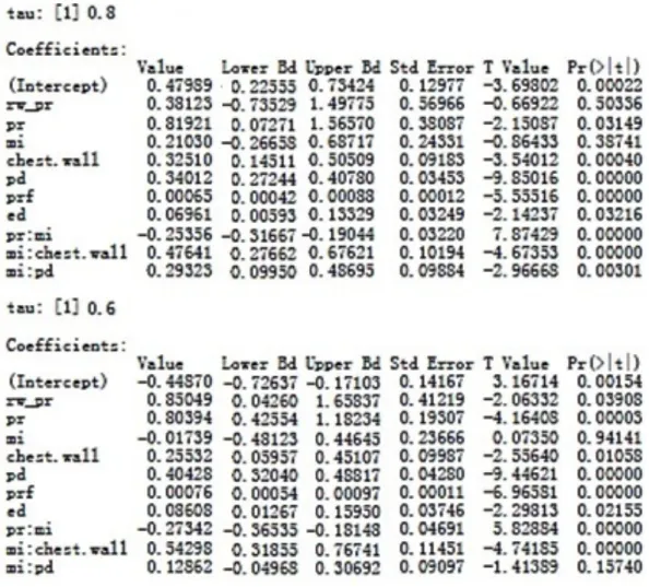
4.2 Summary table of estimates for pr+pr*mi+chest.wall*mi+pd*mi+prf+ed ...38
4.3 Summary table of estimates for pr*mi+chest.wall*mi+pd+prf ...41
4.4 Summary table of estimates for pr*mi+chest.wall*mi+pd+prf+beam ...43
4.5 Summary table of LASSO and SCAD screening results for a sequence of τ’s ...49
4.6 Summary of λ vs. τ ...50
4.7 Summary table of 2-way interaction for LASSO ...52
4.8 Crq results of the full model at 𝜏 =0.5, and R=10 ...53
List of Figures
4.1 Plot of Powell predictions where y = lesion depth and x = threshold wave length for
two different starting value ...28
4.2 Prediction Made Using Portnoy’s and Peng and Huang’s estimates ...29
4.3 Plot of 𝜆 versus coefficients of standardized variables ...31
4.4 Plot of 𝜆 versus coefficients of original variables (none standardized) ...32
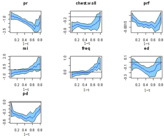
4.5 Confidence band of the base model pr+chest.wall+prf+mi+freq+ed+pd, where x-axis is 1-τ and y-axis is the coefficient t ...34
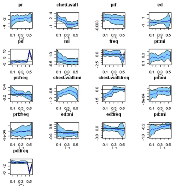
4.6 Confidence band of (pr+chest.wall+prf+ed+pd)*(mi+freq), where x-axis is 1-τ and y-axis is the coefficient ...35
4.7 Confidence band of pr+pulse+pr*mi+chest.wall*mi+ chest.wall*rw pr+pd*mi+prf +ed, where x-axis is 1-τ and y-axis is the coefficient ...36
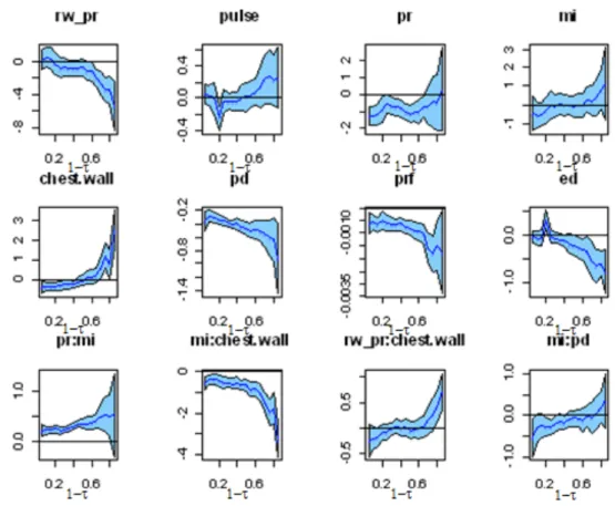
4.8 Confidence band of rw_pr+pr*mi+chest.wall*mi+pd*mi+prf+ed, where x-axis is 1-τ and y-axis is the coefficient ...37
4.9 Confidence band of pr*mi+chest.wall*mi+pd+prf, where x-axis is 1-τ and y-axis is the coefficient ...40
4.10 Confidence band of pr*mi+chest.wall*mi+pd+prf+beam, where x-axis is 1-τ and y- axis is the coefficient ...42
4.11 Plot of 𝜆 versus coefficients of the standardized variables for SCAD ...45
4.12 Confidence band of mi+ pr+ pd+chest.atten, where x-axis is 1-τ and y-axis is the coefficient ...46
4.13 Histogram of chest.atten ...47
4.14 Example of widening of Confidence Band ...48
4.15 Summary of λ vs. τ ...51
List of Abbreviations
CLAD Censored Least Absolute deviationsLASSO Least Absolute Selection and Shrinkage Operator SCAD Smoothly Clipped Absolute Deviation
animal Animal ID
chest.wall Thickness of Chest Wall to Lung in mm
chest.atten Attenuation Coefficient in dB/mm
freq Ultrasound Frequency in MHz
pd Pulse Duration in mu-sec
prf Pulse Repetition Frequency
ed Exposure Duration
beam Width of Beam at Focus
pr Calculated in Vivo Acoustic Pressure at the Lung Surface
Chapter 1
Introduction
Many variable selection methods are available for linear regression but very little has been developed for quantile regression, especially for the censored problems. This study will look at the possibilities of utilizing some existing penalty variable selection methods on censored quantile regression problems.
1.1 Censored Regression Quantile
Censoring occurs when the recorded data is only partially known or occurs outside the range of measuring instrument (Chay et. Al, 2001). Many statistical methods can be used to fit models with censored data. The traditional statistical analysis used the maximum likelihood procedures. This method requires specification of the error distribution and a wrong error distribution will cause this method to generate an estimate that is not consistent (Honore and Khan, 2002).
The Tobit model in context of quantile regression has been of great interest among the researchers. It is also known as the censored normal regression model and has the following structural equation:
𝑦!∗ = 𝑥!!𝛽!+𝜖!, 𝑖 =1,…,𝑛 , [1]
where ϵ!~𝑁 0,𝛿! ,𝑦∗is a latent variable that is observed for values greater than C and censored otherwise. The observed y is defined by the following measurement equation
y! = 𝑦𝐶∗ 𝑖𝑓 𝑦∗ >𝐶
! 𝑖𝑓 𝑦∗≤ 𝐶 . [2]
In the ultrasound safety example below, the data set is censored at 0 lesion depth. Thus, we have
y! = 𝑦0 𝑖𝑓 𝑦∗ 𝑖𝑓 𝑦∗∗≤>00 . [3]
A required feature of Tobit model is that the censoring points are known for the dependent variables for all the observations. If the distribution of the error term is indeed Normal and homoscedastic, then it is straightforward to derive and maximized the likelihood function. If these two conditions are unsatisfied then the Tobit estimator will be inconsistent (Yu and Stander, 2007). It is obvious these assumptions put stringent restrictions on the application of this model. Nevertheless, it is interesting to study how the Tobit estimator differs from the more generalized estimator such as the Portnoy (2003) censored quantile regression estimator, which requires less assumptions. A small example on the neonate data set was performed. And the results showed that the estimations from these two methods are very similar.
Powell (1986) proposed the censored least absolute deviations (CLAD) estimation method. He noted that the estimator for the Tobit model solves
min ! ! ! 𝜌! 𝑌! −max {𝑦! !,𝑋 !!𝛽} ! !!! , [4]
Where ρ! 𝜆 =[𝜃−𝐼 𝜆< 0 ]𝜆 is the check function and 𝐼(∙) is the usual indicator function (Buchinsky and Hahn, 1998). Although, Powell's work opened a new window to solving censored problems, with error distribution that is nonnormal or heteroskedastic, his estimator has some disadvantages. The most notable disadvantage is that the objective function is not convex
by Fitzenberger (1996) helps solve this problem, but still doesn’t ensure convergence to a local optimum. It should be noted when implementing the Powell's method using the QUANTREG package in R, one can specify the starting value of the coefficients. In the present study, we looked at both the Powell estimator and Portnoy estimator (Portnoy, 2003). When running the Powell method in CRQ program, the default starting regression quantile estimate on the Neonate lung data set had a strong influence on the resulting estimate of the coefficients. The majority of the runs could not be completed and, hence, failed to generate coefficient estimates for any of the quantiles. The reason for such failure is unclear. It is suspected that the large ratio, approximately 0.5, of the censored and uncensored data points may have caused this failure, where the censored value is 0. Because of the problem we experienced with the Powell’s estimator, it was decided that it is not suitable for this particular data and will not be further used in our study. Our focus is put on the Portnoy estimator that has more general censoring assumptions, which we will discuss in more detail later on.
In the situation when censored values are not known for each observation, it is common to model the censoring as random. Under the assumption that 𝑦! and 𝐶! are conditionally independent given 𝑥!, there are two commonly used random censored quantile regression estimators: the Portnoy (2003) and Peng and Huang (2008) estimators. Both are incorporated in the CRQ program in R (Koenker, 2008). Recently it has been proven that in large sample environment Peng and Huang's and Portnoy estimator are asymptotically equivalent (Limin Peng, 2009). The present study focuses on the Portnoy estimator. One computational advantage of using Portnoy estimator is it is relatively simpler to retrieve the weights used in this method than in other methods. These weights are crucial when using the LASSO variable selection method (Tibshirani, 1996).
When presented with one-sample problem where y! =𝑚𝑖𝑛 (𝑦!∗,𝑐!) , Kaplan-Meier can be used to estimate the quantile function instead of the survival function. One method of computing Kaplan-Meier estimator is to recursively reweights the estimates by redistributing the mass of the censored data point, P[Y! >𝐶!], to the observations above Ci. The fundamental problem is finding P[Y! > 𝐶!]. In terms of quantile regression, this is equivalent to finding the 𝜏 which x!!𝛽(𝜏) crosses Ci. The weights can then be incorporated into the parametric approach described by Koenker and D'Orey (1987). The disadvantage of reweighting the estimate is the monotonicity condition weakens, where even under the one-sample setting, it is possible to have censored observations crossed by estimate quantile and which will cause it to have negative residuals (Koenker and D’Orey, 1987). In his 2003 paper, Prof. Portnoy introduced an effective method that is similar to the approach described in Koenker and D'Orey (1987), but solves the "recrossing"' problem by computing 𝛽(𝜏) along a grid of 𝜏 values.
From the detailed algorithm described in Portnoy (2003), one can simply retrieve the weights from the crq.fit.por program by adding the 𝜏!!𝑠 of the crossed censored data points, named splittau in the R-code, to the list of returned variables within the algorithm of the crq.fit.por program. The crossed censored data points that correspond to split τi and are smaller than τ will have its weight split into two parts:
1) 𝑤! 𝜏 = !!!!!!!
!, 𝑓𝑜𝑟 𝑥!,+∞ , [5]
2) 1−𝑤! 𝜏 , otherwise, [6]
where𝜏> 𝜏!. As summarized in Koenker (2008), the intuition of this method is that the quantile depends solely on how much mass is below and how much is above. Assigning 1−𝑤! 𝜏 to
some arbituarily large response and 𝑤! 𝜏 to 𝜏! ensures that the weighted response corresponds to the 𝜏!! conditional quantile.
An advantage of the weighted censored regression quantile approach is that one can, in principal, use any kind of penalty in combination with the censor-weight modified regression quantile. This is especially helpful computationally, because crq program in the quantreg package (Koenker, 2012) already allows certain penalties. In this study, two penalized variable selection methods are of primary interest. One is the least absolute selection and shrinkage operator (LASSO) Tibshirani (1996) and the other is the smoothly clipped absolute deviation (SCAD) Fan and Li (2001).
1.2 Penalized Variable Selection Methods
The well-known traditional model selection criteria, such as AIC and BIC, are infeasible for variable selection in high-dimensional data. When a large number of predictors are introduced at the initial stage, these methods become prone to suffer from instability and they involve heavy computations (Breiman, 1996). Two feasible alternative methods for model selection of high-dimensional problems are LASSO and SCAD. Both methods are penalized maximum likelihood estimators that can jointly minimize the residual sum of squares plus penalty and can avoid large variation, which occurs in estimating complex models. The computational simplicity of LASSO has attracted much attention of many users. Its computational complexity is similar to just one linear regression. But its dubious consistency property makes it tricky to use (Zou and Li, 2008). Zhao and Yu (2003) showed that if an irrelevant covariate is strongly correlated with the significant covariates, then no matter how large the data set is, LASSO will most likely fail to
distinguish the true covariates. Furthermore, Zhao and Yu showed that there exists an almost necessary and sufficient condition, the irrepresentable condition, for which the consistency of LASSO will hold true. The SCAD estimator of Fan and Li (2001) was introduced to improve the performance. Many scientists have studied its asymptotic properties and have found that under appropriate conditions, the SCAD estimator is consistent for variable selection. In addition, its asymptotic distribution and its 'oracle' property can be computed when the SCAD estimator is consistent.
The LASSO and SCAD methods have been adapted for use when dealing with weighted-regression. The process of retrieving the censor related weights from the Portnoy's algorithm and feeding these weights along with the response and predictors into the algorithm of these methods provides an approach for penalized censored quantile regression. Although, the asymptotic consistency of the LASSO and SCAD methods and the Portnoy estimator (Portnoy and Lin, 2010) have been established, the main theoretic hurdle of this study is to prove that the consistency property does indeed extend to the weights, such that the transformed response and predictor variables will still hold the asymptotic consistency properties of the LASSO and SCAD results.
This paper is organized as follows. In Chapter 2, we describe the proposed penalized quantile regression variable selection method. In Chapter 3, we present the large sample theory. In Chapter 4, we examine the high-dimensional data set using the proposed variable selection method. Finally, in Chapter 5, we provide the computing algorithm used in the penalized quantile regression.
Chapter 2
Penalized Quantile Regression for
Variable Selection
There are limited tools for performing variable selection in quantile regression. Although in this study we focuses on censored quantile regression, our method can be applied to all quantile regression problems. The basic idea of our method is 1) variable screening; 2) Fine tuning of variables using backwards selection and bidirectional regression. We tested LASSO and SCAD variable screening method for the censored problem. This is more complicated than regular quantile regression, but using Portnoy method, the censored data is simplified into a weighted problem. Then manually applied the backwards and bidirectional regression for fine-tuning of variable and their interactions terms.
The crq function offered in the quantreg package (Koenker, 2012) fits conditional quantile regression model for censored data. User can choose from three methods: Powell (1986), Portnoy (2003), Peng and Huang (2008). We are interested in random censoring in particular the Portnoy’s method. When the Portnoy’s method is specified in crq, this signals the program to call the function crq.fit.por. The original crq.fit.por command in R does not return the index of the crossed censored data points and the crossed τ. But these two pieces of information are vital in the calculation of weights generated by the Portnoy’s random censored quantile regression method at the crossed data points. To retrieve the above information we simply add the variable
quantile that corresponds to Isplitth crossed censored response, to the list of the returned variables defined in crq.fit.por algorithm. We name this new version of crq.fit.por that returns these two additional variables, the crq.por.tsp. This new version will replace the original crq.fit.por when Portnoy’s method is called in crq function.
The algorithm for calculating the split weights is rather straightforward. First, we retrieve Isplit and T. We then duplicate the entries identified by Isplit for which τi < τ. This creates the additional entries for us to assign the split weight. Third, overwrite the response of the duplicated entry with a much larger value, say 100. Since the quantile can be determined by only knowing the sign of the residual, therefore, assuming the response is the arbitrary value of 100 is equivalent to knowing the true observation because the sign of their residual are the same. Hence, a part of the weight of the crossed censored observation is distributed to the true observation, even though the true value is unknown. Finally, assign the correct weights according to equation [4] and [5]. All other entries that are uncensored or uncrossed have the weight of 1. Multiplying this vector of weights to the response vector and the X matrix (this X
matrix includes the duplicated entries with the edits mentioned above), transforms the problem into a weighted regression problem.
Please note the crq function was designed to handle only right random censoring problems until recently. Majority of the analysis were performed before this update of crq. Originally to compute the left censoring problem we had to change the sign of the response variable. Although this tricks the program to compute left censoring as the right censoring problems, it also replaces 𝜏 with 1-τ. Therefore, the plots given in this paper actually has x-axis equal to 1-τ rather than τ, but the discussion will assume left censoring. So small responses will
correspond to small 𝜏, and large responses will correspond to large 𝜏. The most recent version of rq package now appears to allow specification of left censoring.
In this study we used two popular variable screening methods: the L1 norm LASSO penalty of Tibshirani and the L1 norm SCAD penalty of Fan and Li. These two methods have conveniently built-in functionality in the quantreg package. The algorithm for analyzing the weighted regression problem using these two methods is rather straightforward. Users only need to plug in the weighted x and y values calculated following the above method into the function rq.fit.lasso and rq.fit.scad and specify the 𝜆 value. The penalty parameter 𝜆 determines how much shrinkage is done.
The solution to the LASSO with L1 penalty can be given as
𝛽!"##$ =𝑎𝑟𝑔min
!
𝑌−𝑋𝛽 !+𝜆 𝛽
!! , [7]
where λ≥ 0 is the shrinkage parameter (Tibshirani, 1996). When λ is large this becomes an ordinary least squares linear regression problem. But for λ that is sufficiently small, it would be possible to shift through the variables and separate the significant variables from the rest. It has been shown (Zhao and Yu, 2006) that there exists an irrepresentable condition, which depends mainly on the covariance of the predictor variables. And LASSO selects the true model consistently if and (almost) only if the predictors that are not in the true model are “irrepresentable” (in a sense to be clarified) by predictors that are in the true model. The quantile regression version of LASSO is
𝛽!"##$ =𝑎𝑟𝑔min
!
The smoothly slipped absolute deviation (SCAD) was first proposed by Fan and Li (2001). The penalty is given by
𝛽!"#$ 𝜆 = 𝑎𝑟𝑔min ! ! ! 𝑌−𝑋𝛽 !+𝜆 𝑝 !( 𝛽! ! !!! ) . [9]
The solution to the SCAD penalty is given as
𝛽!!"#$ = 𝛽! −𝜆 +𝑠𝑖𝑔𝑛 𝛽! 𝑖𝑓 𝛽! < 2𝜆; !!! !!!!"#$ !! !" !!! 𝑖𝑓 2𝜆 < 𝛽! ≤ 𝑎𝜆; 𝛽! 𝑖𝑓 𝛽! >𝑎𝜆 [10]
It has been shown (Huang and Xie, 2007) that under appropriate conditions, the SCAD-penalized least squares estimator is consistent for variable selection. The estimators of nonzero coefficients have the same asymptotic distribution as they would have if the zero coefficients were known in advance. The quantile version of the SCAD is
𝛽!"#$(𝜆) =𝑎𝑟𝑔min ! ! !𝜌! 𝑤𝑌,𝑤𝑋𝛽 +𝜆 𝑝!( 𝛽! ! !!! ) . [11]
Oracle results are available for the SCAD method. Because of the oracle properties of SCAD, it was found the SCAD penalty method outperforms the LASSO in terms of model error (Zou and Li, 2009). But because SCAD is a nonconcave penalty, it is much more difficult to compute than LASSO. Furthermore, Hall and Lee and Park (2009) showed that the bootstrap-based penalty choice for the LASSO can achieve oracle performance.
LASSO and SCAD is different mostly in its penalty term. But similarly the computation of penalties only involve 𝛽, do not work with the weights for the censored data directly. This makes the problem much simpler to handle and relatively easier to prove its consistency. Chapter 3 discusses the proof of consistency in large sample. In general, one would expect
LASSO and SCAD results to differ in varying degrees. It is expected their result to be most similar at the quantile with most data, i.e. the median, and most different when there is least amount of data, i.e. the boundaries. In Chapter 4, we will compare screening results at different levels of 𝜏 for a specific case study.
How to choose the right 𝜆 can be tricky. For example, when λ is too large LASSO becomes an ordinary least squares linear regression problem. When λ is too small, significant variables cannot be separated from the rest. Instinctively we feel this threshold 𝜆 is likely subjected to the magnitude of variables and the specific dataset. To remove the magnitude effects, we can simply standardize the variables. The dataset effect on 𝜆 is much more complicated to remove if not entirely impossible. But if we can determine a certain pattern in threshold 𝜆 and 𝜏, then we could possibly generalize a method for selecting the appropriate threshold 𝜆. But this requires tremendous amount of data. We begin by looking at the lung dataset, which will be elaborated in Chapter 4.
There are some disadvantages in using LASSO and SCAD in crq. Particularly, when dealing with higher order models, performing LASSO and SCAD can be a tedious task. For example, one cannot simply multiplying the variable together to create the interaction term in the command object of crq.LASSO, which is common privilege in other crq fitting tools. Hence, the variables must be manually multiplied together and added to the data frame. So the 2-way variable is treated as a new variable. This can be cumbersome when you have many 2-way variables in your model. Most importantly, when model gets too lengthy, crq can take a very long time to run, and in our experience it may fail to converge. Instead of putting all the 2-way variables in one large model with its main effects, we propose two ways to analyze a complex model. First, screen the main effects model and manually perform bidirectional regression by
entering the 2-way interactions. Second, screen each main effect along with all its 2-way interaction individually, then, combine the results and manually perform a backward regression to fine-tune the model. Surprisingly, two methods produced very similar results. Though, the backward regression may be simpler to program into a function that can be applied automatically in qr.
Chapter 3
Large Sample Theory for Censored
Penalized Quantile Regression
In this chapter we will establish consistency of the proposed censored penalized quantile
regression estimator to provide theoretical backing for the use of the procedure in practice. It has been shown under appropriate conditions, the SCAD-penalized least squares estimator is
consistent for variable selection (Huang and Xie, 2007). In addition, we also know the model selection consistency of the LASSO is highly dependent on some irrepresentable condition (Zhao and Yu, 2006). The asymptotic distributions of both methods have been derived and shown to perform consistent modal selection (Potscher and Leeb, 2009). Therefore, in principle, since individual methods of the proposed penalized regression quantile estimator has been proven to be asymptotically consistent under certain conditions, it seems natural for the combination of the LASSO or SCAD with Portnoy estimator to produce an asymptotically consistent results. In this chapter we will show, in finite dimensional problem with large sample, our variable selection method produces consistent results and the asymptotic normal distribution holds.. Penalized and unpenalized censored quantile regression differs only by a penalty term. Naturally, the consistency proofs are very similar. We have adapted previous results from Portnoy and Lin (2010) to establish the consistency for the finite dimensional penalized censored problem. In addition, as an analogy to Portnoy and Lin (2010) work, the asymptotic distribution theory also
holds for penalized version. First, define the subgradient of the penalized quantile loss function Ψ!!!! as follows: Ψ!!!! 𝑤 !,𝛽 𝑡! = 𝑥! ! !!! {𝐼 ∆!=1 𝜓 𝑌! −𝑥!!𝛽 𝑡 ! ,𝑡! + 𝐼 ∆!=0 × 𝑤!! 𝑡! 𝜓 𝐶!−𝑥!!𝛽 𝑡 ! ,𝑡! + 1−𝑤!! 𝑡! 𝜓 𝑌∗−𝑥!!𝛽 𝑡! ,𝑡! }+ !!!!𝑝!! 𝛽 𝑡! [12]
where 𝜓 𝑢,𝜏 =𝜏−𝐼 𝑢 ≤0 , and Y* is sufficiently large value larger than all observed and fitted values. As described in Koenker (2008), the gradient conditions impose a bound of the form Ψ! 𝑤,𝑏 =𝑂 1 𝑎𝑡 𝑏= 𝛽 𝑡 (uniformly in k), as long as 𝑥! remain bounded (see
condition (5) below).
Here we will restate the conditions needed for the results in Portnoy and Lin (2012) plus 4 additional conditions (8)-(11):
(1) All conditions restrict to 𝜖 ≤𝜏 ≤𝑚𝑖𝑛 𝜏,1−𝜖 where 𝜏 is the largest identifiable 𝜏 -value. Furthermore, there is no censoring below 𝑥′𝛽 𝜖 . Hence, 𝛽 𝜖′ can be computed as an
unweighted regression quantile for 𝜖′ < 𝜖 with probability tending to one. (2) (xi,Yi,Ci) are i.i.d.
(3) Yi and Ci are conditionally independent given xi and have conditional distribution functions
Fiand Gi, respectively.
(4) The conditional densities 𝑓! 𝑥!!𝛽 𝑡 and 𝑔
bounded derivatives (with respect to t) on 𝜖 ≤ 𝜏≤ 𝑚𝑖𝑛 𝜏,1−𝜖 , and are strictly positive on this set.
(5) ∥xi∥ has bounded support.
(6){t1,...,tM}is a grid with mesh δn = cnn−a for some a with ¼ < a < ½ and cn → c (with c > 0).
(7) The design matrix, X, satisfies n-1X′X → A, where A is invertible. (8) {xi} is consider fixed.
(9) 𝛽 𝑡 is boundely differentiable on 𝜖 ≤𝜏 ≤𝑚𝑖𝑛 𝜏,1−𝜖 .
(10) 𝑝′! ≤ 𝑐𝜆! , where 𝑐 >0. (11) There is a constant 𝑐∗ such that 𝜆
! satisfies 𝜆! ≤ 𝑐∗ 𝑑!,!𝛿! where 𝑑!,! and 𝛿! are defined in Theorem 3.1.
Inductive Proof of Consistency
From this point on, we will follow the exact steps of Portnoy and Lin (2012) inductive proof of consistency.
THEOREM 3.1. Let 𝛽! ≡ 𝛽 𝑡! !,…,𝛽 𝑡
! ! be the right censored penalized quantile estimator along the grid 𝜖 = 𝑡! < 𝑡! <⋯ <𝑡! ≤ 𝑚𝑖𝑛 𝜏,1−𝜖 (where 𝜏 is the largest identifiable τ-value). Under Conditions (1)–(7), we have
𝛽 𝑡! −𝛽 𝑡! ≤2𝑟!𝑛!!𝑑
where M =o(n1/2), 𝑑!,! =𝑅! 𝑛 1+2𝑟!𝑟!𝐸!∗𝛿
! 𝑘!!with 𝐸!∗ = 𝑂! 1 , and 𝑅! = 𝑂! 1 andis
defined by: 𝑅! = 𝑛!!/!𝑚𝑎𝑥
! Ψ!!! 𝑤!,𝛽 𝑡! + 𝐸!,! . Here, 𝜆! =𝑂(𝑑!,!𝛿!) , Ψ!!! is the defined by Equation (1)and r1 and r2 are defined by Equations (2) and (3); and we show that 𝐸!,! =𝑂! 𝑛!/!log𝑛 uniformly in k, where 𝐸
!,! is defined by Equation (4). Recall that
𝛽 𝑡! is the true regression quantile along the same grid, and δn = O(n−a) is defined in Condition (6).
Remark: note that since 𝑑!,!𝛿! =𝑂(𝑛 !
!!!) (by condition (6)), the rate at which 𝜆! can tend to
infinity is controlled by the constant, a. Under the hyposthesis of Theorem, the rate can grow at least algebraically (since a < 1/2), but can grow at a rate no faster than n(1/4).
Proof Let CIk = {i : Yi = Ci and 𝑚𝑎𝑥 𝜏!,𝜏! ≤𝑡!} be the index set of the crossed censored observations.
We shall use mathematical induction to show that for any k = 1, 2, . . . , M,
𝜏!−𝜏!
!∈!!! ≤ 𝑑!,! , and 𝛽 𝑡! −𝛽(𝑡!) ≤ 2𝑟!𝑛!!𝑑!,! . [13] First let k = 1, 𝛽 𝑡! is the penalized quantile estimator at t1 by applying the usual censored regression quantile. Since we are dealing with a left censoring problem, then there are no censored data to the left of t1, hence, it can be treated as an uncensored quantile regression problem. Furthermore, it is known that 𝛽! 𝑡! −𝛽(𝑡!) =𝑂! 𝑛!!/! by Theorem 3.1 in
Koenker (2008), where 𝛽! 𝑡! is the uncensored quantile regression estimator at t1. Therefore, 𝛽 𝑡! −𝛽(𝑡!) = 𝑂! 𝑛!!/! ≤ 2𝑟
Using the fact that there are no censored data to the left of 𝑋′𝛽 𝑡! , it follows the 𝜏! and 𝜏! must be greater than t1. Hence, !∈!!! 𝜏! −𝜏! =0 , and Equation [13] is true k=1.
As shown in Portnoy and Lin (2010), assume that for k=1, Equation [13] is true, then the bound for the difference between the estimated weights and the true weights at tk+1th quantile can be expressed as follows:
𝑤! 𝛽!,𝑡!!! −𝑤! 𝛽!,𝑡!!! !
!!! ≤ !!!!! 𝑑!,! 1+𝐸!𝛿! . [14]
Define 𝜂! 𝜃,𝛽 𝑡!!! = Ψ!!! 𝑤 𝛽!,𝑡!!! ,𝜃 −Ψ!!! 𝑤 𝛽!,𝑡!!! ,𝛽 𝑡!!! , with Ψ!!! given by Equation (1). From the proof of Lemma 4.1 in He and Shao (1996), we can see that for any constant C*>0, there is a constant A2>0, such that for large enough values of A1>0 and n,
𝑃 𝑚𝑎𝑥 !!!!! 𝑠𝑢𝑝 !: !! !!!! !!∗!! ! ! 𝜂! 𝜃,𝛽 𝑡!!! −𝐸!𝜂! 𝜃,𝛽 𝑡!!! >𝐴!𝑛 ! !log𝑛 ≤𝑀𝐴!𝑒!!!!. Let En,l be defined as 𝐸!,! = 𝜂! 𝜃,𝛽 𝑡!!! −𝐸!𝜂! 𝜃,𝛽 𝑡!!! [15] on 𝜃: 𝜃−𝛽 𝑡!!! ≤ 𝐶∗𝑛! !
! . As shown in Portnoy and Lin (2010) proof of Theorem 2.1, for none penalized censored problem En,l = Op(n1/4 log n) uniformly in l. For clarification purposes let the superscript P symbolize the penalty affect. Note, ! 𝑝!!
!!! is not a function of y, therefore, adding a penalty in the regression will not change this limiting behavior. This is shown below.
𝐸!,!! = Ψ!!!! 𝑤 𝛽 !,𝑡!!! ,𝜃 −Ψ!!!! 𝑤 𝛽!,𝑡!!! ,𝛽 𝑡!!! −𝐸! Ψ!!!! 𝑤 𝛽 !,𝑡!!! ,𝜃 −Ψ!!!! 𝑤 𝛽!,𝑡!!! ,𝛽 𝑡!!! =Ψ!!! 𝑤 𝛽!,𝑡!!! ,𝜃 −Ψ!!! 𝑤 𝛽!,𝑡!!! ,𝛽 𝑡!!! −𝐸! Ψ!!! 𝑤 𝛽!,𝑡!!! ,𝜃 −Ψ!!! 𝑤 𝛽!,𝑡!!! ,𝛽 𝑡!!! + 𝑝!! 𝜃 ! !!! − 𝑝!! 𝛽 𝑡 !!! ! !!! −𝐸! 𝑝!! 𝜃 ! !!! − 𝑝!! 𝛽 𝑡 !!! ! !!! =𝜂! 𝜃,𝛽 𝑡!!! −𝐸!𝜂! 𝜃,𝛽 𝑡!!! =𝐸!,!. Since Ψ!!!!=Ψ !!!+ !!!!𝑝!! it follows the Ψ!!!! 𝑤 𝛽 !,𝑡!!! ,𝜃 =Ψ!!! 𝑤 𝛽!,𝑡!!! ,𝜃 + !!!!𝑝!! 𝜃 . [16]
Using the results from Portnoy and Lin (2010) proof of Theorem 2.1, Ψ!!!! 𝑤 𝛽
!,𝑡!!! ,𝜃 can
be expressed in the following form:
𝑤!−𝑤! 𝐼 𝐶! <𝑥!!𝜃 𝑥 ! !"#!! +Ψ!!! 𝑤 𝛽!,𝑡!!! ,𝛽 𝑡!!! +𝑋!𝑉𝑋 𝜃−𝛽 𝑡 !!! +𝐸!,! + !!!!𝑝!! 𝜃 . [17]
Note that, uniformly in l (and with w denoting 𝑤 𝛽!,𝑡!!! ),
(a) Ψ!!! 𝑤,𝜃 =𝑂 𝑛!/! ,
(b) ! 𝑤! −𝑤! 𝐼 𝐶! < 𝑥!!𝜃 𝑥!!𝐼 ∆!=1 ≤ ! 𝑥! 𝑤!−𝑤!
≤ 𝑥! !!!!!!!𝑑!,! = 𝑂! 𝑛!/! ,
Note: 𝑥! has a bounded support. Hence, in (b) we assume 𝑥! is the max of all possible 𝑥! .
(c) Ψ!!! 𝑤,𝛽 𝑡!!! = 𝑂! 𝑛!/! ,
(d) 𝐸!,! =𝑂! 𝑛!/!log𝑛 , and (e) 𝜆!"# 𝑋′𝑉𝑋 !! ≤ 𝑎!!𝜆
!"# 𝑋′𝑋 !! ≤ 𝑎!𝑛!!,
where 𝑉!! ≥𝑎 >0 , for some a1 > 0 uniformly in i. Because of condition (7), the right side inequality of (e) is true.
The convex property of Ψ!!! 𝑤,𝜃 and SCAD penalty !! 𝑝!! 𝜃
!!! allows for Ψ!!!! 𝑤,𝜃 to be
convex. Note, q! is the number of non-zero coefficients and p’ is the derivative of the SCAD penalty. It follows the above results may be used without changing the gradient condition of
𝜃: 𝜃−𝛽 𝑡!!! > 𝐶∗𝑛!!/! , under the condition that a large enough C* is chosen (Theorem 2.1 in Koenker (2008)). Replace 𝜃 with 𝛽 𝑡!!! in Equation [17] and solve for 𝛽 𝑡!!! −
𝛽 𝑡!!! −𝛽 𝑡!!! = 𝑋′𝑉𝑋 !! 𝑤 ! −𝑤! 𝐼 𝐶! < 𝑥!!𝜃 𝑥! !"#!! +Ψ!!! 𝑤 𝛽!,𝑡!!! ,𝛽 𝑡!!! −Ψ!!!! 𝑤 𝛽 !,𝑡!!! ,𝛽 𝑡!!! +𝐸!,! + 𝑝!! 𝜃 !! !!! 𝛽 𝑡!!! −𝛽 𝑡!!! ≤ 𝑎!𝑛!! 𝑤! −𝑤! 𝐼 𝐶! < 𝑥!!𝜃 𝑥! !"#!! + Ψ!!! 𝑤 𝛽!,𝑡!!! ,𝛽 𝑡!!! + Ψ!!!! 𝑤 𝛽 !,𝑡!!! ,𝛽 𝑡!!! + 𝐸!,! + 𝑝!! 𝜃 !! !!!
Using (b) and Equation [16] 𝛽 𝑡!!! −𝛽 𝑡!!! ≤𝑎!𝑛!! 𝑥 ! 𝑤! −𝑤! ! + Ψ!!! 𝑤 𝛽!,𝑡!!! ,𝛽 𝑡!!! + Ψ!!! 𝑤 𝛽!,𝑡!!! ,𝛽 𝑡!!! + 𝐸!,! +2 𝑝!! 𝜃 !! !!!
absorbed into 𝑂! 𝑛!/!log𝑛 of En,l. Likewise 𝑥
! can be absorbed in a1. Hence, we can drop Ψ! 𝑤,𝑏 from the inequality. Furthermore, using the bound for ! 𝑤! −𝑤! in Equation [14] it follows 𝛽 𝑡!!! −𝛽 𝑡!!! ≤𝑎!𝑛!! 1−𝜖 𝜖! 𝑑!,! 1+𝐸!𝛿! + + Ψ!!! 𝑤 𝛽!,𝑡!!! ,𝛽 𝑡!!! + 𝐸!,! +2 𝑝!! 𝜃 !! !!!
In the Theorem 3.1, it is defined that 𝑅! =𝑛!!/!𝑚𝑎𝑥
! Ψ!!! 𝑤!,𝛽 𝑡! + 𝐸!,! . As
defined in Portnoy and Ling (2010) Equation 18, 𝑟! = 𝑎!!!!!! . We can rewrite the inequality in terms of r1 and Rn 𝛽 𝑡!!! −𝛽 𝑡!!! ≤𝑟!𝑛!!𝑑 !,! 1+𝐸!𝛿! +𝑎!𝑛!!𝑅! 𝑛+𝑎!𝑛!!2 𝑝!! 𝜃 !! !!!
By the definition of dl,n ,we know that 𝑑!,! > 𝑅! 𝑛. In addition, when 𝜀 ≤0.5 then r1 > a1, so we get the following equation.
𝛽 𝑡!!! −𝛽 𝑡!!!
≤ 𝑟!𝑛!!𝑑
!,! 1+𝐸!𝛿! +𝑟!𝑛!!𝑑!,! +2𝑟!𝑛!! 𝑝!! 𝜃 !!
!!!
𝛽 𝑡!!! −𝛽 𝑡!!! ≤2𝑟!𝑛!!𝑑 !,! 1+𝐸!𝛿! +2𝑟!𝑛!! 𝑝!! 𝜃 !! !!! [18]
Next, we will look at how the penalty term can be combined in the first term of the inequality. We know by definition 𝑝!! 𝜃 = 𝑝′ 𝜆
!,𝑎 and 𝑝′ 𝜆!,𝑎 <𝑐𝜆!, where c is some positive
constant. Then
𝑝!! 𝜃 <𝑞
!𝑐𝜆!
!! !!!
By the hypothesis of the theorem, 𝜆! satisfies
𝑞!𝑐𝜆! ≤𝑐∗ 𝑑
!,!𝛿!
for some constant c* (since 𝑞≤𝑑 and c and d are bounded). We can achieve an upper bound for 𝑝!! 𝜃 !! !!! by 𝑝!! 𝜃 !! !!! ≤𝑐∗ 𝑑 !,!𝛿!
Now, Equation [18] can be written as
𝛽 𝑡!!! −𝛽 𝑡!!!
≤2𝑟!𝑛!!𝑑
!,! 1+ 𝐸! +𝑐∗ 𝛿!
[19] If we let 𝐸!+𝑐∗ =2𝑟
!𝑟!𝐸!∗ , then Equation [19] can be written as follows:
𝛽 𝑡!!! −𝛽 𝑡!!!
≤2𝑟!𝑛!!𝑑!,! 1+2𝑟!𝑟!𝐸!∗ 𝛿! =2𝑟!𝑛!!𝑑!!!,!
Hence 𝐸!∗ = 𝐸
!+𝑐∗ /2𝑟!𝑟!.
Lets look at the upper bound for !∈!!!!! 𝜏! −𝜏! . We can use the none-penalized results given in Portnoy and Lin (2010) Equation [19], because its calculation does not involve any penalty term, hence, their results holds true for the penalized quantile regression as well.
𝜏! −𝜏! !∈!!!!! ≤𝑑!,!+2𝑟!𝑟!𝑑!,! 1+𝐸!𝛿! 𝛿! ≤ 𝑑!,! 1+2𝑟!𝑟!𝐸!∗𝛿 ! =𝑑!!!,! [20] where 𝐸!∗ = 1+𝐸 !𝛿!, 𝑟! = 𝑥! !!(!! !!! !) !!!(!!!!!! ).
Now, in order to satisfy both Equation [19] and [20] we define
𝐸!∗ = 𝑚𝑎𝑥 !!!!∗
Note, this result is derived from Portnoy and Lin (2010) Equation [20], where adding a constant to the first term will not change the overall asymptotic behavior.
To deal with asymptotic theory, let 𝛽∗ be the estimate based on the selected variables, and let 𝜃 be the estimate based on the true model. By consistency, 𝛽∗ =𝜃 with probability tending to 1.
Thus, 𝛽∗−θ = 𝑂
!(𝑎!), where 𝑎!is an arbitrary sequence tending to zero. Taking 𝑎! tending
to 0 faster than 1/ 𝑛, the equivalence of asymptotic distribution for 𝛽∗ and 𝜃 follows from Slutzky’s theorem. Portnoy and Lin (2010) provide an asymptotic Gaussian representation for the process 𝑛 (𝛽∗(𝑡)−𝜃(𝑡)) . Though there is no closed form expression for the asymptotic covariance matrix, this provides the following theorem covering the right-censored estimator and justifying the use of the bootstrap for asymptotic inference.
Theorem 3.2. Under the hypotheses of Theorem 3.1, for any 𝜏 between 𝜖 and 𝑚𝑖𝑛 𝜏,1−𝜖 ,
𝑛 (𝛽∗(𝑡)−𝜃(𝑡)) converges in distribution to multivariate normal distribution with mean 0 and
fixed covariance matrix.
For details on the proof and computation of the estimated covariance matrix see Portnoy and Lin (2010).
Chapter 4
Case Study
Ultrasound has assumed great importance in medical imaging and it is presumed to be safe at typical diagnostic levels. The safety of ultrasound depends on the level of exposure. Back in the 1980s, this level of exposure was much more conservative and fairly safe. But in 1991 the US government relaxed its regulation allowing the intensity level of ultrasound used to scan the in utero fetus to increase almost eight times over the level that had been allowed previously. The ultrasound (measured in time average-intensity) generated by equipment for obstetrics is about 1000-fold of the level back in the 1980s (Toms, 2007)! In addition, the use of ultrasound has expanded in the prenatal ultrasounds from the 2D to now 4D imaging (Merritt, 1989). So the natural question to ask is how safe is the ultrasound these days?
Ultrasound induced lung hemorrhage is one topic that has been studied extensively since the 90's(Zachary and O'Brien 1995; Baggs et al. 1996; Raeman et al. 1996; Dalecki et al. 1997a, 1997b; O'Brien and Zachary 1997; O'Brien et al. 1001a; Zachary et al. 2001). Different animal-based studies were performed in the interest of investigating the association between the occurrence and size of the US-induced lung hemorrhage, and the factors such as the US pressure, frequency, beam width species and age of animal. The logistic regression analysis and Gaussian-Tobit analysis were used. It was found that the ultrasound-induced lung hemorrhage in adult rats
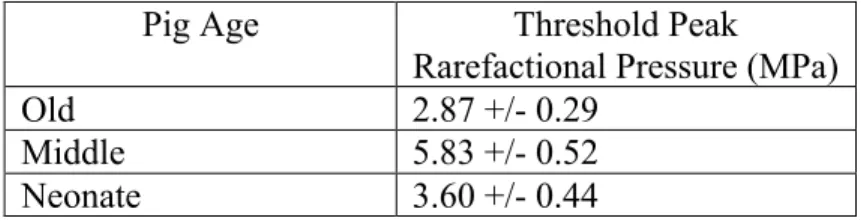
strongly influenced by situ peak rarefaction pressure (acoustic pressure) and beam width and their interaction (O’Brien et al, 2001). In addition, ultrasound frequency was found to be not significant in the same experiment (O’Brien et. al, 2001). But it was determined using the logistic regression analysis and Gaussian-Tobit analysis methods on the pig data, the occurrence of the lesion is a function of age and the results are summarized in Table 4.1.
Pig Age Threshold Peak
Rarefactional Pressure (MPa)
Old 2.87 +/- 0.29
Middle 5.83 +/- 0.52
Neonate 3.60 +/- 0.44
Table 4.1: Summary of pig age versus threshold peak rarefactional pressure in the Gaussian-Tobit Analysis of pig data (O’Brien et. al, 2003).
It can be seen in Table 4.1, the lesion threshold is greatly affected by the physiology of the lung (O’Brien et. al, pig 2003). In conclusion, structural differences among mammalian species studied are independent of the biological mechanism that causes ultrasound-induced lung damage; therefore, it is reasonable to speculate the mechanisms that cause lung hemorrhage in laboratory animals may also damage human beings especially small children and patients with pulmonary disorders. It is extremely important to be able to estimate thresholds of mechanisms that cause ultrasound-induced damage (O’Brien et. al, 2007).
The pig data used in this example is the same as the data set used in O’Brien paper (2003). It is a high-dimensional data set with 4 animal related variables 7 instrument-setting variables. The variables are defined and listed below.
Animal related variables: species
animal = id of the animal
chest.wall = thickness of chest wall to lung in mm
chest.atten = attenuation coefficient in dB/mm
Instrument settings:
freq = ultrasound frequency in MHz
pd = pulse duration in mu-sec
prf = pulse repetition frequency
ed = exposure duration
beam = width of beam at focus
pr = calculated in vivo acoustic pressure at the lung surface
mi = mechanical index
Variable mi is closely related to pr, hence it is not necessary to include both variables. However, out of curiosity we did keep mi in the bidirectional regression analysis.
We begin our analysis using Portnoy’s random censoring estimator. Using crq.fit.por algorithm, the information needed to calculate the weights of each observation can be retrieved as described in Chapter 2. Using these weights we can transform a censored quantile regression problem into a weighted quantile regression problem. These weights are used in the weighted regression part of the LASSO variable screening method. The coefficients estimates generated from the LASSO can be plotted and used for visual diagnostics.
4.1 Penalized Model Screening - LASSO
We begin our analysis by first testing Powell’s, Portnoy’s, and Peng and Huang’s methods on a much smaller data set called the neonates. Our goal was to become familiar with the RQ package through replicating the analysis that was previously done by Simpson et. al using the Tobit method (2004). Unfortunately, we had experienced many problems with the Powell’s estimator. We believe these problems are related to the selection of the starting values (Portnoy, 2010). As seen in Figure 4.1, quantiles generated using the Powell’s estimator are crossed and varies drastically with the starting value.
Figure 4.1: Plot of Powell predictions where y = lesion depth and x = threshold wavelength for two different starting value.
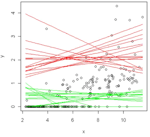
Portnoy’s and Peng and Huang’s estimator were both successfully computed. These estimates were very close to the estimate of Tobit’s method. Figure 4.2 is a plot of the prediction of lesion depth computed using the Portnoy’s and Peng and Huang’s and Tobit’s methods.
Figure 4.2: Prediction Made Using Portnoy’s and Peng and Huang’s estimates, where green and yellow lines are Portnoy’s prediction, blue and red are Peng and Huang’s estimates, and Orange and black are Tobit’s estimate.
2
4
6
8
10
0
1
2
3
4
x
y
The data set used for the rest of our study is the pig lung data set that was once studied by O’Brian et. al (2003). It is much larger than the neonate data set mentioned above, and consists of 11 variables and 2483 entries. There are 3 response variable: lesion, depth, and area. The variable lesion is the censoring variable that takes on value of 0 and 1, where 1 means lesion depth is greater than 0, and 0 means no lesion. There were precisely 3 observations with either 0
lesion but a depth greater than 0 or the opposite scenario. These points were corrected via R by changing the value of lesion to match the depth. The response variable area measures the surface area of the lesion. Since it serves the same purpose as depth, which both measure the ultrasound-induced hemorrhage, only depth was used in our analysis. Furthermore, we noticed the observed values of variables vary significantly in magnitude. To avoid any magnitude effects on the estimation calculation, these variables were standardized using mean and standard deviation before performing any analysis,.
The preliminary analysis begins with analyzing the full model consists of all variables minus variables species and animal. Intuitively, these two variables incorporate information that pertains to specific species and animals. It is our goal to develop a generalized model that can be used for any species and animals. Hence, we hope to find some combination of the variables other than species and animal that could help explained the lesion depth. In addition, including these two variables in the model will cause the crq program to fail. It is likely due to singularity of the X matrix. After a model is fitted using crq.por.tsp, we can then retrieve the Isplit and T.
We begin our analysis at τ = 0.5. The median is a good starting point since the most abundant information is generally at the median; therefore, the analysis would potentially give us the most accurate model. Note, τ is used in the calculation of the split weights at the crossed censored observations. These adjusted weights help redistribute the probability to the unknown
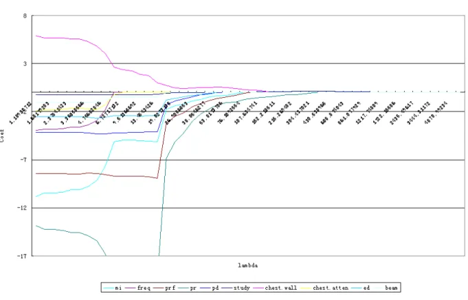
true responses as well as the censored responses. Then LASSO method is used to generate coefficients for the weighted problem. A sequence of 𝜆‘s was examined. For each𝜆a set of 𝛽
was recorded. Figure 4.3 and Figure 4.4 are plots of𝜆versus 𝛽. In Figure 4.3, the coefficients were calculated based on the standardized variables.
Figure 4.3: Plot of 𝜆 versus coefficients of standardized variables.
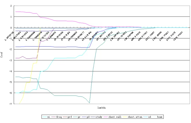
Figure 4.4 is the plot of 𝜆 versus coefficients of original variables for none standardized data. As expected, the shape of the LASSO tree is similar, but the variables are separated better, where the threshold 𝜆 is slightly smaller for the standardized data. In addition, there is less tail affect, hence easier to decipher the more significant variables.
Figure 4.4: Plot of 𝜆 versus coefficients of original variables (none standardized).
From the above LASSO tree plots, it is noticeable that the estimates calculated based on the standardized variables actually shrink to 0 at a different rate than the none standardized. The calculation based on the original data yields the most significant 7 variables to be (in the order of importance) as follows: Pr, ed, chest.wall, prf, mi, pd, study. Note: beam is not listed. Although this variable remained in the model for all the 𝜆′𝑠, its estimated coefficient is consistently very small, relatively speaking. When all the variables are standardized, the order of importance is listed as following: pr, chest.wall, prf, mi, freq, pd, and ed. When the variables are standardized, the variable beam shrinks to 0 much quicker than before. One question arises, is the magnitude of the estimates influential in variable selection, in the since that does the shrinking rate overrules the magnitude difference? Intuitively it seems likely a variable with coefficient
stays in the model for all 𝜆’s, this is not an indication that this variable is more important than others. In addition, LASSO is not built to detect interaction affects. But one may be able to pick up some signs of possible interactions by looking at the variable shrinking behavior. If a variable initially shrinks to 0 quickly but later reenters the model when some other variable falls out, then this could be an indication that interaction may exist between these variables. Finally, the selected base model using standardized variables with no two-way interaction is present in R language as follows:
cr q( Sur v( - dept h, l es i on) ~ pr+chest.wall+prf+mi+freq+ed+pd, met hod="Por ", dat a = Dat as et ) . Only 7 variables were selected because the 8th significant variable is study, which similar to species and animals, it incorporates information of a combination of instruments used during the experiment. It is our goal to generalize the model so that it can apply to any combination of instrument settings. Therefore, we would like to remove experiment specific variables such as
study, and hence, replace it with more important instrument variables.
We have performed the LASSO variable screening method on the pig lung data set. The SCAD method is another screening method that we can easily access in R. We will compare the results from these two methods later in the paper.
4.2 Extension of Portnoy Estimator – Inference Based Refinement of Screened
Variables
We begin by examining the confidence plot of the crq fit shown in Figure 4.5. Please note the x-axis is 1-τ not τ. In our following discussion, τ is always the left censoring quantile.
Figure 4.5: Confidence band of the base model pr+chest.wall+prf+mi+freq+ed+pd, where x -axis is 1-τ and y-axis is the coefficient.
Clearly the estimates of freq, mi, and ed all cross 0 for significant part of the quantiles spectrum. Variables freq and mi seems to be insignificant for large τ’s, and ed is insignificant for small and large τ’s. We will investigate to see if this is due to interaction between the variables. Note, ed
should be kept as an main affects since it is significant for τ = 0.5. To investigate for possible two-way interaction of freq and mi with other terms, we examine the following model
cr q( Sur v( - dept h, l es i on) ~ (pr+chest.wall+prf+ed+pd)*(mi+freq), met hod="Por ", dat a = Dat as et ) .
Figure 4.6 is the plot of the two-way interaction model. From the plot we can see the confidence band for pr, chest.wall, prf, ed, and pd have changed significantly.
Figure 4.6: Confidence band of (pr+chest.wall+prf+ed+pd)*(mi+freq), where x-axis is 1-τ and
y-axis is the coefficient.
Estimates of chest.wall, prf, ed, and pd are now mostly insignificant. And mi and freq are now insignificant for almost the entire spectrum of τ. What’s interesting is the interaction of
chest.wall * mi is significant and chest.wall * freq interaction is also significant but only for large
τ’s. Furthermore, the addition of 2-way interactions removed all the effects of ed. Note, 1 /
surface. Although, freq is not significant in the above model, the product of the wavelength and the acoustic pressure may hold potential to reveal some interesting relationships. We define
rw_pr to be the product of wavelength and acoustic pressure. In addition, prf * ed is the acoustic pressure pulse, pulse, which could also be important in explaining the response. Next we examine the model
cr q( Sur v( - dept h, l es i on) ~ pr+pulse+pr*mi+chest.wall*mi+chest.wall*rw pr+pd*mi+prf+ed, met hod="Por ", dat a = Dat as et ) .
Figure 4.7 is the plot of the confident bands for the above model with the transformed variables and additional two-way interactions.
Figure 4.7: Confidence band of pr+pulse+pr*mi+chest.wall*mi+ chest.wall*rw pr+pd*mi+prf+ed , where x-axis is 1-τ and y-axis is the coefficient.
From the plot you can see the interaction term rw_pr * chest.wall and the main affect term pulse
are mostly insignificant. Removing the other 2 terms and keeping rw_pr by itself, we reduce down to the following model:
cr q( Sur v( - dept h, l es i on) ~ pr+rw_pr+pr*mi+chest.wall*mi+pd*mi+prf+ed, met hod="Por ", dat a = Dat as et ) .
The results are plotted in Figure 4.8. It should be noted the confidence band widen for pd, prf,
and ed, in particularly for small 𝜏’s, but the significance of the variables remained the same .
Figure 4.8: Confidence band of rw_pr+pr*mi+chest.wall*mi+pd*mi+prf+ed, where x-axis is
Removing the rw_pr*chest.wall did not penalize the model significantly. The significant variables remain significant with small changes in their P-value. More detail is given in Table 4.2. In addition, the estimate for rw_pr crosses 0 for large τ’s. Its P-value is given in the following table. In addition, ed and mi * pd are still insignificant for almost the entire spectrum of τ. Its unlikely these two variables will appear in the final model. Furthemore, the interaction term mi*pd are mostly insignificant but it is highly significant as main effects; therefore, it is necessary to include pd and mi as a main effects in the final model.
Table 4.2 (cont.): Summary table of estimates for pr+pr*mi+chest.wall*mi+pd*mi+prf+ed.
Table 4.2 shows the P-value for each variable. Its shown rw_pr has P-value of 0.50 at τ = 0.8, , and becomes more significant as τ decreases. Since we are more interested in high τ values the variable rw_pr may be removed. In addition, at τ=0.8, ed has a P-value of 0.032 and its P-value increases as τ decreases. Even at its prime of τ=0.8, ed is not highly significant, it may be beneficial to remove this variable from the model. Removing these terms will further reduce the model down to
The result of this reduced model is plotted in Figure 4.9. The confidence band changes are quite noticeable for most variables. Variables pr , mi, pd, and pri:mi show most improvement. In particularly, the bands are narrower than before for large τ values.
Figure 4.9: Confidence band of pr*mi+chest.wall*mi+pd+prf, where x-axis is 1-τ and y-axis is the coefficient.
Table 4.3 tabular summary of the estimates for pr*mi+chest.wall*mi+pd+prf. The variables are most significant for 1-τ = 0.8. Chest.wall becomes insignificant for smaller 1-τ values. Since its interaction term is significant, it will remain in the model. Note, pr*mi shows signs of decrease in significant for 1-τ = 0.2.
Look at Table 4.3, it is clear each variable in this new model is highly significant with an exception of chest.wall. But since mi*chest.wall is highly significant, chest.wall will remain in the final model.
The 7 variable model is reduced down to pr*mi+chest.wall*mi+prf +pd. To see if this model has the best fit, we compare to a slightly larger model. We chose to introduce the variable
beam to the model because it is the 8th significant variable screened using LASSO.
Figure 4.10: Confidence band of pr*mi+chest.wall*mi+pd+prf+beam, where x-axis is 1-τ and
It is easy to see in Figure 4.10 that beam is highly significant for all τ’s except when near 1. Table 4.4 shows even at tail regions beam is still highly significant. The two-way interactions of
beam were tested but none were significant. In addition, 9th significant variable, chest.atten, was also added to the model but it crashed crq program. It is possible that this may be the result of singularities. Finally, I conclude the best-fitted model has the following variables:
pr*mi, chest.wall*mi, pd, prf, beam.
It is interesting to note, that one way to examine the validity of a model is by looking at the number of quantiles can be fitted. A "`bad"' model is unable to generate coefficient estimates for a large spectrum of τ’s. The model selected above was able to fit τ ranging from 0.88 to 0.01 in increments of 0.01. It may even be possible to fit τ’s less than 0.01. Hence we are confident, our final model is one of the best-fitted model for this data set.
4.3 Penalized Model Screening - SCAD
Similar to LASSO, the SCAD variable screening method is also build into the RQ package. The weights are generated the same way as for the LASSO method in Section 4.2. The weighted response and variables are then feed into SCAD as we’ve done for LASSO. The results are surprisingly very different than the LASSO findings.
Figure 4.11 is the plot of 𝜆 versus coefficient estimates based on the standardized variables. Just from the first glance, we notice the behavior of the estimates is noticeably different than LASSO.
The variables drop off to 0 where in LASSO they asymptotically approach 0. The advantage of this clear-cut result allows the variable selection to be less subjective. Furthermore, variables are essentially split into two groups at 𝜆 =300: 1) mi, pr, pd, and chest.atten that never approach 0, therefore, remain highly significant for all 𝜆’s, 2) variables either already shrunk to 0 before 𝜆
reach 300 or remain very close to 0 for 𝜆 >300.
Figure 4.11: Plot of 𝜆 versus coefficients of the standardized variables for SCAD.
Next, we discuss the difference of the base model chosen via SCAD vs. LASSO. Surprisingly,
chest.atten is most significant for SCAD method. Figure 4.12 is the plot of confidence band of the variables estimates for the following base model
cr q( Sur v( - dept h, l es i on ) ~mi+ pr+ pd+chest.atten, met hod = "Por ", dat a = Dat as et ) -30 -25 -20 -15 -10 -5 0 5 Coef lambda
Tunning Parameter vs Coef (SCAD)
mi freq prf pr
pd study chest.wall chest.atten
Figure 4.12: Confidence band of mi+ pr+ pd+chest.atten, where x-axis is 1-τ and y-axis is the coefficient.
The chest.atten is highly significant for the most of τ’s in SCAD results, especially the large 𝜏 ‘s of interest. This is a strong contrast to the LASSO findings. If you recall, chest.atten was added to the LASSO final model as a check for the best fit. When it was included in the final model
pr*mi, chest.wall*mi, pd, prf, beam the crq program crashed. It appears the variable chest.wall
with chest.atten may have caused the singularity in the X matrix. These two variables are both animal variables measuring characteristics of the animal lung. Hence, it is possible they are correlated.
comparison let’s be consistent with the LASSO and focus on the 7 significant variables. These variables are: chest.atten, pr, mi, pd, beam, prf, and ed (in the order of significance). If you recall, we initially selected the following variables using LASSO method: pr, chest.wall, prf, mi,
freq, pd, and ed (in the order of significance). The differences are chest.atten replaced the
chest.wall and beam replaced freq in the SCAD results. Figure 4.13 is the plot of chest.atten
histogram. Notice chest.atten takes on rather discrete values; this may also be a reason why LASSO crashed. We investigated this possibility by tethering 𝜆 with a very small random number. But this did not solve the crash of LASSO. Hence, evidence points towards the possibility of correlation.
Figure 4.13: Histogram of chest.atten.
Histogram of chest.atten chest.atten F re q u e n cy -1.0 -0.5 0.0 0.5 1.0 1.5 2.0 2.5 0 200 400 600 800 1000 1200