Technological University Dublin
Technological University Dublin
ARROW@TU Dublin
ARROW@TU Dublin
Conference papers
School of Computing
2011-08-24
A Framework for Generating Data to Simulate Application Scoring
A Framework for Generating Data to Simulate Application Scoring
Kenneth Kennedy
Technological University Dublin, [email protected]
Sarah Jane Delany
Technological University Dublin, [email protected]
Brian Mac Namee
Technological University Dublin
Follow this and additional works at: https://arrow.tudublin.ie/scschcomcon
Part of the Databases and Information Systems Commons, Design of Experiments and Sample Surveys Commons, and the Other Statistics and Probability Commons
Recommended Citation
Recommended Citation
Kennedy K., Delany S.J. & Mac Namee B. (2011) A Framework for Generating Data to Simulate Application Scoring. In: Credit Scoring and Credit Control XII, Conference Proceedings, Credit Research Centre, Business School, University of Edinburgh doi:10.21427/D70P50
This Conference Paper is brought to you for free and open access by the School of Computing at ARROW@TU Dublin. It has been accepted for inclusion in Conference papers by an authorized administrator of ARROW@TU Dublin. For more information, please contact
[email protected], [email protected], [email protected].
This work is licensed under a Creative Commons Attribution-Noncommercial-Share Alike 3.0 License
A Framework for Generating Data to Simulate Application Scoring
K. Kennedya,∗, S.J. Delanyb, B. Mac Nameea
aSchool of Computing, Dublin Institute of Technology, Ireland bDigital Media Centre, Dublin Institute of Technology, Ireland
Abstract
In this paper we propose a framework to generate artificial data that can be used to simulate credit risk scenarios. Artificial data is useful in the credit scoring domain for two reasons. Firstly, the use of artificial data allows for the introduction and control of variability that can realistically be expected to occur, but has yet to materialise in practice. The ability to control parameters allows for a thorough exploration of the performance of classification models under different conditions. Secondly, due to non-disclosure agreements and commercial sensitivities, obtaining real credit scoring data is a problematic and time consuming task. By the provision of publicly available artificial data, credit scoring is opened to the wider data mining community. This in turn could help enable greater participation, promote replicable experimental findings, and give rise to solution proposals to outstanding credit scoring problems.
To ensure that our framework is sufficiently grounded in reality, data distributions are generated using a troika of sources: demo-graphic information from the Central Statistics Office, Ireland; housing statistics published by the Irish Government Department of the Environment, Heritage and Local Government; and a profile of loan defaulters developed using a recent report published by a credit rating agency. By engaging with a credit scoring expert we select characteristics that are typical of most application scorecard models including, amongst others: age, income, loan value, and occupation. Through user controlled settings the conditional prior probabilities of the characteristics can be adjusted over time to simulate differing scenarios. In order to assign class labels to the generated data a credit risk score is estimated based on the non-linear interactions between various characteristics. Based on the desired number of defaulters a cut-offscore is placed on this monotonic ordering of credit scores to distinguish between those likely to repay and those likely to default on their financial obligation. The classification complexity is controlled by adding user-defined random Gaussian noise.
After discussing the desirable characteristics of artificial data we describe a pseudo-random data generator for credit scoring and provide illustrations on how the framework can be used to generate population drift.
Keywords: Data Mining, Supervised Classification, Artificial Data, Simulation, Model Risk, Population Drift, Application Scoring
1. Introduction
The ongoing debt hangover affecting many private house-holds (see Haldane, 2010) along with the fragile recovery in the financial system underlines the role of credit scoring in de-termining borrowers’ access to credit. The term credit scor-ing is used to describe the process of evaluating the risk an applicant poses of defaulting on a financial obligation (Hand and Henley, 1997). The objective is to assign borrowers to one of two groups: good or bad. A member of the good group is considered likely to repay their financial obligation. A member of the bad group is considered likely to default on their financial obligation. The merits of credit scoring are well established in the literature and include reducing the cost of credit analysis, enabling faster credit decisions, closer moni-toring of existing accounts, and prioritising collections (Brill, 1998). As credit scoring is essentially a discrimination problem
∗
Correspondence: Kenneth Kennedy, K107A, School of Computing, Dublin Institute of Technology, Kevin St., D8, Ireland
Email address:[email protected](K. Kennedy)
(good or bad), one may resort to the numerous classification techniques that have been suggested in the literature. Many of these classification models are derived from statistical meth-ods, non-parametric methmeth-ods, and artificial intelligence-based approaches (Leeet al., 2005).
For an academic researcher, obtaining real credit scoring data with which to evaluate approaches is a problematic and time consuming task. This is due, in part, to commercial sensitiv-ities and quite often acquiring real credit scoring data from a financial institution is simply an untenable task. It is therefore reasonable to regard the credit scoring research community, like many other research communities, as one that lacks a data shar-ing culture. This is not meant as a critique of the community itself but rather an acknowledgment of the barriers in sharing data.
In this paper we aim to address this issue by proposing a framework to generate artificial datasets that can be used in the design and assessment of classification techniques for credit scoring. This in turn could help enable: (i) greater participation and diversified perspectives; (ii) replicable experimental
find-ings; (iii) increased creativity and solution proposals; and (iv) reduce time spent extracting, transforming and loading data.
To ensure that our framework is sufficiently grounded in re-ality, datasets are generated using a troika of sources: demo-graphic information from the Central Statistics Office, Ireland (CSO, 2010); housing statistics published by the Irish Gov-ernment Department of the Environment, Heritage and Local Government, or DEHLG, (DofE, 2008); and a profile of loan defaulters developed using market data from Moody’s Global Credit Research (Moodys, 2010). By engaging with a credit scoring expert we select features that are typical of most ap-plication scorecard models including, amongst others, age; in-come; loan value; and occupation. In order to assign class la-bels to the generated data a credit risk score is estimated based on a set of non-linear, multi-feature rules designed in consul-tation with a credit scoring expert. Based on the desired de-fault rate a cut-offscore is placed on this monotonic ordering of credit scores to distinguish between those likely to repay and those likely to default on their financial obligation. The classifi-cation complexity is further controlled by adding random Gaus-sian noise with a mean of zero and a user adjustable standard deviation to this score.
The rest of the paper is organised as follows. In Section 2 we highlight how many of the datasets used in the literature are not publicly available, as well as the over-reliance on the few publicly available datasets. The advantages and motiva-tions for using artificial data are discussed in Section 3. Section 4 presents our artificial data generation framework. The valid-ity of our framework is assessed in Section 5. A demonstration of how the framework can be used to simulate population drift is provided in Section 6. Finally, future work and conclusions are presented in Section 7.
2. Background
In credit scoring, over the last decade numerous studies ex-amining the performance of various models used to construct credit scorecards have been produced, (see West, 2000; Lee
et al., 2002; Baesenset al., 2003; Hsieh, 2005; Onget al., 2005; Xiaoet al., 2006; Huanget al., 2007a; Zhanget al., 2007; Tsai and Wu, 2008; Nanni and Lumini, 2009; Zhou et al., 2010; Khashman, 2010; Wang et al., 2010; Kennedy et al., 2010; Chen et al., 2011). The popularity of such studies is moti-vated, in part, by the widely accepted view that the proposed or novel method can be accepted only if it is demonstrably su-perior to existing methods (Japkowicz and Shah, 2011). Many experts question the premise that a new methodology, using the same characteristics of the data as used by existing methods, produces a superior performance (see Hand, 2006b). A further concern is that the data used in these studies originates from two sources: (i) the Australian and German datasets which are pub-licly available from the University of California Irvine (UCI) Machine Learning Repository (Asuncion and Newman, 2007); and (ii) private datasets obtained from financial institutions.
The UCI repository serves several important functions (Salzberg, 1997). The repository allows published results to
be checked and through comparison with existing results re-searchers can assess the plausibility of a new algorithm. A number of researchers (Salzberg, 1997; Saitta and Neri, 1998; Soares, 2003; Martenset al., 2011), however, caution against over-reliance on the UCI repository as a source of research problems. The repository is cited as a potential source of over-fitting. Researchers familiarity with datasets from the repos-itory may influence them to design algorithms that are tuned to the datasets (Drummond, 2006). It is beneficial that re-searchers do not over-rely on the UCI repository, preferably multiple data sources should be used. For example, Keogh and Kasetty (2003) demonstrate how experimental results are greatly effected by the choice of test data and describe this phe-nomenon asdata bias which is defined as“the conscious or unconscious use of a particular set of testing data to confirm a desired finding.”As a result researchers often ignore the prob-lem of trying to understand under which conditions an algo-rithm works well or not (Soares, 2003).
Another issue with datasets from the UCI repository raised by researchers is that the datasets are not truly reflective of the real-world and only capture a small subset of all the situ-ations that can arise in real-world situsitu-ations (Saitta and Neri, 1998; Drummond and Holte, 2005; Drummond and Japkowicz, 2010). The Australian and German credit application datasets also contain very different class distributions and the overall size of the datasets is not representative of sizes that arise in practise. Such differences are likely to be an artefact of how the datasets were constructed, which in turn raises questions about how the data was collected (Drummond and Japkowicz, 2010). The inclusion of certain characteristics raises questions about the current relevancy of the UCI data. For example, in an age of the ubiquitous mobile phone, the use of a telephone charac-teristic in the German dataset is questionable. The assumption that the sample is random needs to be treated with caution and we should be careful not to derive too much from experimental results using such datasets (Drummond and Holte, 2005). As always it is desirable to use data derived from a richer source of diversity that captures a wider aspect of the world. Obtain-ing real-world data is a source of great frustration for those re-searchers who lack the necessary resources.
Fischer and Zigmond (2010) describe a number of factors impeding the sharing of data within academia, which are reiter-ated below.
Negative Career Impact. The need to publish is important to a researcher’s career and datasets used may be part of a long-term endevour from which an individual could generate multi-ple publications. If a researcher is required to share data after their first publication the opportunity to generate further pub-lications may be reduced if a better funded and resourced re-search group obtains the data. In fact, sharing data with others can be regarded as a means of providing them with a competi-tive advantage on publication by eliminating the need to collect and clean data. Another factor to consider is the lack of in-centives to share data (Blumenthalet al., 2006; Teeters et al., 2008). Currently there are no metrics for sharing data which can be considered when awarding grants, promotions, or
recog-nition (citing the source of the dataset does alleviate this prob-lem somewhat). Also, sharing data requires personnel to pre-pare the material for distribution. This in turn could result in reputational damage to the originator by a failure to have ex-perimental results replicated based on poorly prepared data.
Limited Resources. Sharing data may require extra resources to convert it into an accessible form for other researchers. This reduces the time and money available to the originator to pursue their own research activities. Certain datasets may require up-dating and maintenance, once a researcher has completed their work it may be no longer feasible to store the data.
Property Rights and Legal Issues. As previously stated, legal and commercial reasons may prohibit the researcher from shar-ing data. Customer confidentiality, for example, is of the utmost importance for any financial institution. While with a single anonymised dataset it may not be possible to identify a particu-lar individual, customer identity may be compromised through the combination of multiple datasets. A further restriction is that often data collected for one purpose may not be used for another purpose without requesting additional permission from the customers involved themselves.
Bergkamp (2002) believes that European Union data protec-tion laws impose an onerous set of requirements on the data processor as data privacy is considered a “fundamental right” (EU, 1995). It is argued that restricting the flow of data between business and research, consumers ultimately receive outdated, lower quality products and services at higher prices (Bergkamp, 2002).
The authors are of the opinion that the above barriers will re-main in place for the foreseeable future. Principally this is due to a lack of incentives, for the originator, to share data and the overly stringent requirements of data protection laws. Without the provision of publicly available datasets though, credit scor-ing will remain closed to the wider data minscor-ing community.
In domains where access to real-life data may simply be unattainable and to overcome the aforementioned limitations currently associated with machine learning data repositories, we contend that the use of artificial data is acceptable. It should be stressed that the data must be generated in the correct man-ner and be sufficiently grounded in reality in order to avoid the danger of investigating imaginary problems.
One may argue that as the UCI and other data repositories evolve over time, the quantity, quality, and variety of datasets will improve (Japkowicz and Shah, 2011). An advantage ar-tificial data has over real-life data is the flexibility afforded to the manipulation of various parameters used in the evaluation process. This allows the researcher to design specific experi-ments aimed at evaluating algorithms’ performance under cer-tain conditions of interest in a relatively precise manner (Scott and Wilkins, 1999; Japkowicz and Shah, 2011).
The practise of using research data generated by simulation is common in many other domains e.g. atmospheric and geophys-ical sciences (Reichleet al., 2002), medicine (Robinsonet al., 2009), fraud detection (Lundinet al., 2002), and intrusion de-tection (Lippmannet al., 2000a,b). The next section examines
the applicability of artificial data to research problems, most notably in the credit scoring domain.
3. Artificial Data
Artificial data can be defined as ‘‘data that are generated by simulated users in a simulated system, performing simu-lated actions”(Lundinet al., 2002). The termssynthetic data,
dummy data, andsimulated dataare also used to describe arti-ficial data.
In the following section we highlight previous work in arti-ficial data generation along with its use in credit scoring. Fol-lowing this we identify the characteristics of authentic data that should be present in artificial data.
3.1. Artificial Data: Previous Work
Researchers have often experimented with artificial data to test the efficacy of various classification algorithms across dif-ferent data distributions. For example, Kim (2010) generated 324 simulated classification problems to evaluate the perfor-mance of the decision tree, neural network, and logistic regres-sion techniques. Markham and Rakes (1998) used artificial data to compare linear regression and artificial neural network mod-els across 20 datasets varying the sample size and the variance in the error. Scott and Wilkins (1999) describe two artificial data generators, one based on the multi-variate normal distribu-tion and the other inspired by fractal techniques for synthesising artificial landscapes.
Often artificial data is used when only one class of data is available, i.e. fraud detection, intrusion detection, and fault de-tection. Fraud detection, areas of which involve the screening of credit applications and/or credit card transactions, is closely related to credit scoring. For similar legal and commercial rea-sons it is difficult to obtain authentic fraud datasets. Other than a relatively small automobile insurance dataset used by Phua
et al.(2004) there are no publicly available datasets for studying fraud detection (Phuaet al., 2010). One approach used to ad-dress these data availability shortcomings is by using artificial data which closely matches authentic data. Barseet al.(2003) proposed a five-step artificial data generation methodology that can be used to generate new cases of fraud and variations of known frauds.
Intrusion detection is another domain where artificial data is also routinely used. DARPA (Lippmann et al., 2000a,b) artificially generates network traffic and system call log files from a large computer network along with malicious software attacks. However, several contributions in the literature have highlighted concerns about the authenticity of the DARPA sim-ulations (see McHugh, 2000; Mahoney and Chan, 2003). Other studies that have utilised artificial data to mimic network traffic and malicious intrusions in order to obtain a labelled training set include Debaret al.(1998); Theiler and Cai (2003); Hu and Panda (2004); Bertinoet al.(2005); Steinwartet al.(2005); Abe
et al.(2006). This list is by no means exhaustive but it serves to indicate the widespread use and acceptance of artificial data in the field of intrusion detection.
Fault detection is typically used to detect and identify faults in complex systems, e.g. flight control systems or environmen-tal monitoring systems used in chemical processes. By mon-itoring all the information on a system it is possible to detect quantities that are over-sensitive to malfunctions (also referred to as residuals) (Herediaet al., 2008). Due to safety, environ-mental and financial reasons artificial residual data is often used as an alternative means to introduce a fault into an expensive and complex system. In one such example Samyet al.(2011) use artificial data to simulate multiple sensor failure in an un-manned aircraft vehicle. Refer to Venkatasubramanian et al.
(2003b,c,a) for a comprehensive overview of fault detection. In credit scoring a straight-forward approach used to gen-erate artificial data is to select data points from a multivariate distribution centred at alternate values and with various covari-ance matrices (see Hand and Adams, 2000; Fortowsky et al., 2001). An even simpler approach is to use two univariate Gaus-sian distributions as this allows for visualisation of the model (see Kellyet al., 1999; Hoffmannet al., 2007). Publicly avail-able artificial datasets such as Ripley’s dataset (Ripley, 1994) have also been used (see Martens et al., 2007). Hand (2004) observes that one of the limitations of artificial data is that it usually relates to problems which one would rarely encounter in practice e.g. intertwined spirals or chequerboard patterns. In addition, the previously listed examples of artificial data may miss the data structures typical of credit application data. It is important that generated artificial datasets should be based on reality. A number of participants at a workshop on evalu-ation methods for machine learning (Drummondet al., 2006) espoused an artificial data generation framework which uses a real domain as input and by automated analyses of the input, variations of the dataset that follow some high level character-istics are generated. An example of such an approach is under-taken by Narasimhamurthy and Kuncheva (2007) who propose a framework for generating data to simulate changing environ-ments through the introduction of deformations applied to the data. The deformations are brought about by simulating pop-ulation drift- a term used to describe to changes in the proba-bility distributions of the phenomena under study (Kellyet al., 1999). However the generated data is either two dimensional or, importantly, requires an existing dataset from which to generate the data.
Many specialised dataset generators have been described in the literature. Examples include an IBM dataset generator (Al-maden, 2004) which simulates a retail environment and pro-duces market baskets of goods; andcelsim(Myers, 1999) used in the genome assembly process by generating a user described DNA sequence with a variety of repeat structures along with polymorphic variants. Alaiz-Rodr´ıguez and Japkowicz (2008) simulate a medical domain that states the prognosis of a patient a month after being diagnosed with influenza. Each patient is described using a number characteristics: (i) patient age; (ii) in-fluenza severity; (iii) patient’s general health; and (iv) patient’s social status. Three of the characteristics (age, influenza sever-ity, social status) are completely independent and one charac-teristic (general health) is dependent on two other characteris-tics (age, and social status). The prognosis class depends on
all four characteristics and the data is generated based on user defined prior probabilities for each characteristic. By manip-ulating the prior probabilities for each characteristic the user can simulate various scenarios (e.g. an increasingly virulent in-fluenza outbreak, developing population, or poorer population). A number of general frameworks for generating data also exist (Atzmueller et al., 2006; Melli, 2007), however such general frameworks cannot replicate the rich complexity and intricacies of a specific domain.
To the best of our knowledge no framework exists for gener-ating artificial credit scoring data. The main purpose of our arti-ficial data framework is to provide researchers with a means of creating artificial (but suitably realistic) credit scoring datasets with which to assess the behaviour of classification techniques which can, in turn, serve as an illustration used to help advance some research proposed direction in tool development, as per Liuet al. (2009). The use of artificial data to determine the superiority of some particular classification technique over an-other should be avoided. It is the opinion of the authors that the inherent unpredictability of real-world data cannot be repli-cated using artificial data. One cause of this unpredictability is the structural complexities arising from external and uncaptured circumstances (Scott and Wilkins, 1999). This cannot be repli-cated as structural regularity must be imposed on artificial data in the form of some fixed distributional model (Japkowicz and Shah, 2011). Furthermore, even though unintended, generated artificial data can be biased towards a particular classification technique that is capable of modelling the data more closely than others.
3.2. Properties of Data
As artificial data must be representative of authentic data it is necessary to define the required properties of authentic data. Within the literature, there are many properties that contribute towards data quality. Lindsayet al.(2010) conducted an analy-sis of the literature and found that the most common character-istics of data quality are accuracy, completeness, timeliness, rel-evance, understandability, accessibility and consistency. Data definition is an additional data quality characteristic identified by Baesenset al.(2009).
Data accuracyrelates to the degree of precision of measure-ments of a feature to its true value (Baesenset al., 2009). Listed among the typical causes of poor data accuracy include user input errors and errors in software. Data completenessrefers to the extent to which values are missing in the data (Parker
et al., 2006). Data relevance corresponds as to whether the data addresses the users needs. For example, the selected sam-ple should be as representative of the population for which the data mining model is intended. In credit scoring this is a dif-ficult problem as populations change over time and a certain period of time must elapse before defaulters occur. This in turn requires us to consider data timeliness, which relates to the availability of the data in a user specified time frame. Data understandabilityaddresses how easy it is to comprehend the data. Often, particularly in data mining, it is necessary to trans-form the data into a structure more amenable to data mining techniques. A popular example in credit scoring is to take the
logarithmic transformation of a continuous variable such as in-come which may then improve a data mining technique’s per-formance. Data accessibilityrefers to the ease with which the data can be retrieved when required (Lindsayet al., 2010).Data consistencyrelates to situations in which multiple data sources are used and due to a lack of standardisation, two or more data items may conflict with each other. Data definition refers to the manner in which characteristics have been defined and how they impact the target variable (Baesenset al., 2009). For ex-ample, it is standard practise to discretise a continuous variable (based on some measure such as the weights of evidence) to allow more stable correlation between variables and reduce the over reliance on certain characteristic values.
This section has examined previous work performed in gen-erating artificial data. The limitations of artificial data, in terms of its usefulness in evaluating classification performance, were also highlighted. This section also identified the desired prop-erties of real data, which artificial data should also contain.
4. Methodology
The following section explains the process of generating an artificial credit scoring dataset using our framework. The pro-cess is comprised of two stages: (i) Feature Generation; and (ii) Label Application, each of which will be explained in detail.
4.1. Feature Generation
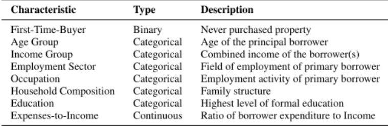
Initially 15 separate characteristics are specified to describe the profile of a mortgage applicant. These characteristics are representative of the Irish mortgage market in 2007. The char-acteristics are selected based on two considerations: (i) the ad-vice of an Irish credit risk expert; and (ii) the availability of offi -cial figures detailing the characteristics. Demographic informa-tion is obtained from the Central Statistics Office, Ireland (CSO, 2010). Housing statistics published by the Department of Envi-ronment, Heritage and Local Government, or DEHLG, (DofE, 2008) are also used to develop a borrower profile. For the class labelling process we utilise a recent Moody’s Global Credit Re-search report (Moodys, 2010), which examined 17 portfolios of securities backed by Irish residential mortgages, profiling Irish loan defaulters. For explanation purposes we split the charac-teristics into two groups: borrower demographics and loan de-mographics. The borrower demographics are described in Table 1. Each of which is explained thereafter.
Table 1: Borrower demographics
Characteristic Type Description
First-Time-Buyer Binary Never purchased property Age Group Categorical Age of the principal borrower Income Group Categorical Combined income of the borrower(s) Employment Sector Categorical Field of employment of primary borrower Occupation Categorical Employment activity of primary borrower Household Composition Categorical Family structure
Education Categorical Highest level of formal education Expenses-to-Income Continuous Ratio of borrower expenditure to Income
First Time Buyer (FTB). This characteristic specifies whether or not the the borrower has previously purchased property. FTB is a binary flag, 1 (New Owner) or 0 (Previous Owner). Based on DEHLG statistics (DofE, 2008) (Ownership status of bor-rowerstab) the prior probabilities are conditional on Location and New Home as displayed in Table 2. Due to a lack of sta-tistical information we do not differentiate between the prior probabilities of properties located outside of Dublin.
Table 2: List of conditional prior probabilities (CPP) for FTB characteristic
FTB Location New Home CPP
1 Dublin 1 0.410 0 Dublin 1 0.590 1 Dublin 0 0.300 0 Dublin 0 0.700 1 Not Dublin 1 0.380 0 Not Dublin 1 0.620 1 Not Dublin 0 0.300 0 Not Dublin 0 0.700
Age Group. This characteristic specifies the age of the primary borrower. The 6 categories are defined based on categories pre-viously employed by the DEHLG (DofE, 2008) (Ranges of ages of borrowerstab). The prior probabilities, displayed in Table 3, are conditional on the FTB characteristic.
Table 3: List of conditional prior probabilities (CPP) for Age characteristic
Age Category FTB CPP 18 - 25 1 0.180 26 - 30 1 0.400 31 - 35 1 0.230 36 - 40 1 0.100 41 - 45 1 0.050 46 - 55 1 0.040 18 - 25 0 0.040 26 - 30 0 0.160 31 - 35 0 0.230 36 - 40 0 0.200 41 - 45 0 0.150 46 - 55 0 0.220
Income Group. The combined annual income of the primary (and secondary) borrower is captured by this characteristic. Based on data contained in the DEHLG housing statistics (DofE, 2008) (Range of income of borrowerstab), 6 categories and prior probabilities (conditional on Location and FTB) are specified in Table 4. In order to validate the data with the Moody’s report (Moodys, 2010) it was necessary to increase the parameter values of the Income Groups as follows: (i)0 to 50,000 is now 40,000 to 60,000; (ii) 50,000 to 60,000 is now60,000 to 80,000; (iii)60,000 to 70,000is now80,000 to 100,000; (iv)70,000 to 80,000is now100,000 to 120,000; (v)
Exceeding 80,000, which has been split into two categories, the first of which120,000 to 150,000; and (vi)Exceeding 80,000, the second of which,150,000+. As per Age Group, an actual income value for each borrower is a randomly generated value between the category parameter values. For the final income category a value is generated using a Pearson distribution with user defined skewness and kurtosis.
Table 4: List of conditional prior probabilities (CPP) for the Income Group categories (Income is listed in ’000)
Category Location FTB CPP 40 - 60 Dublin 1 0.066 60 - 80 Dublin 1 0.148 80 - 100 Dublin 1 0.199 100 - 120 Dublin 1 0.192 120 - 150 Dublin 1 0.200 150+ Dublin 1 0.195 40 - 60 Dublin 0 0.040 60 - 80 Dublin 0 0.062 80 - 100 Dublin 0 0.096 100 - 120 Dublin 0 0.111 120 - 150 Dublin 0 0.300 150+ Dublin 0 0.391 40 - 60 Not Dublin 1 0.173 60 - 80 Not Dublin 1 0.215 80 - 100 Not Dublin 1 0.213 100 - 120 Not Dublin 1 0.157 120 - 150 Not Dublin 1 0.120 150+ Not Dublin 1 0.122 40 - 60 Not Dublin 0 0.090 60 - 80 Not Dublin 0 0.111 80 - 100 Not Dublin 0 0.131 100 - 120 Not Dublin 0 0.129 120 - 150 Not Dublin 0 0.200 150+ Not Dublin 0 0.339
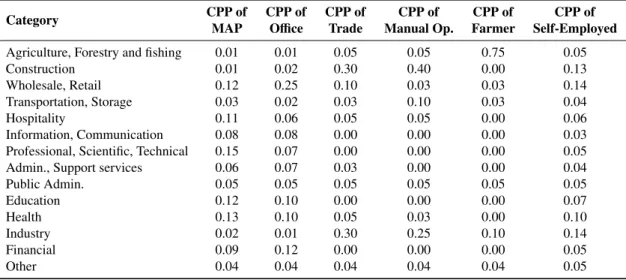
Employment Sector. This characteristic represents the employ-ment activity of the primary borrower. The data is contained in CSO (2010) (2007 column, Table 2.3, pg. 29) whose categories are based on the EU NACE Revision 2 classification (Eurostat, 2008). Modifications have been made by reducing the number of categories to 14, as per Table 5. The prior probability of the characteristic is conditional on the Occupation characteristic.
Occupation. This characteristic attempts to measure the bor-rower’s seniority within their Employment sector. Two sources are used: (i) the CSO Broad Occupational Groupings (CSO, 2010) (2007 column, Table 2.5, pg. 32); and (ii) DEHLG housing statistics (DofE, 2008) (Occupation of borrowerstab). A new group, Self-Employed, has also been added based on Moody’s report (Moodys, 2010). Occupation is split into 6 cat-egories: (i) Manager, Administrator, and Professional (hence-forth MAP); (ii) Associate professional and technical, Cleri-cal and secretarial, Personal and protective service, and Sales (henceforth Office); (iii) Craft and related (henceforth Trade);
(iv) Plant and machine operative (henceforth Manual Op); (v) Other manual operators (henceforth Farmer); and (vi) Self-Employed. The prior probabilities are conditional on Income Group, Location and FTB, as per Table 6.
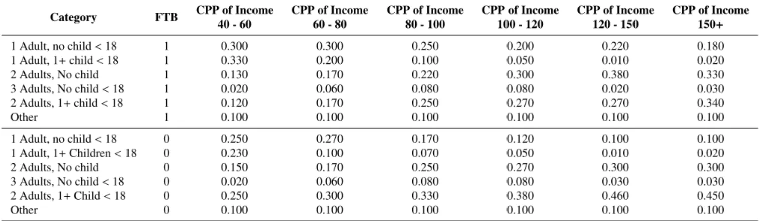
Household Composition. The make-up of the borrower’s household is defined by this characteristic. Household compo-sition is a strong indicator of potential financial outgoings, e.g. childcare fees, university fees. Based on data from CSO (2010) (Table 7.5, pg. 118) the characteristic is split into the following categories: (i) 1 Adult, no child<18; (ii) 1 Adult, 1+child< 18; (iii) 2 Adults, no child<18; (iv) 3+adults, no child<18; (v) 2 Adults, 1+child<18; and (vi) Other. The prior probabil-ities of the characteristic are conditional on Income Group and FTB, as per Table 7.
Education. The Education characteristic captures the highest level of formal education attained by the primary borrower. The characteristic is divided into 7 categories used by the Irish ed-ucational system: (i) Primary or below (PB); (ii) Lower sec-ondary (LS); (iii) Higher secsec-ondary (HS); (iv) Post leaving cer-tificate (PLC); (v) Third level non-honours degree (TLND); (vi) Third level honours degree or above (TLHD); and (vii) Other. The data is based on 2009 data obtained from CSO (2010) (Ta-ble 2.4, pg. 31). The prior probabilities of the characteristic are conditional on Income Group.
Expenses-to-Income. This characteristic represents the stan-dard level of borrower expenditure on commodities and ser-vices. The data is derived from the most recent Household Budget Survey (CSO, 2010) conducted by the Central Statis-tics Office, Ireland. The survey is based on a representative random sample of all private households in the State, thus the results do not distinguish between those households that have recently entered the housing market and those that have been in the market for some considerable time. The following com-modity groups are covered by the survey: Services and other expenses; Transport; Miscellaneous goods; Household durable goods; Household non-durable goods; Housing; Fuel and light; Clothing and footwear; Drink and tobacco; and Food. For the Housing group the mortgage repayments and rent charges have been removed. This is performed as an attempt to minimise the differences between those households that have recently entered the housing market and those that have been in the market for a considerable time.
Each primary borrower is assigned a value representative of the percentage of income spent on household expenses, an Expenses-to-Income ratio. The prior probabilities of the Expenses-to-Income ratio are conditional on Income Group (Table 9) and Household Composition (Table 10). This results in two Expenses-to-Income ratios being generated for each bor-rower: (i) Expenses-to-Income based on Income Group; and (ii) Expenses-to-Income based on Household Composition. When calculating (i) and (ii) for each borrower, a small user-defined random variance taken from a normal distribution is added (subtracted) to (from) each ratio. The average of (i) and (ii) is then calculated for each borrower resulting in a final Expenses-to-Income value.
Table 5: List of conditional prior probabilities (CPP) for Employment Sector categories, which are conditional on the categories of the Occupation characteristic
Category CPP of CPP of CPP of CPP of CPP of CPP of MAP Office Trade Manual Op. Farmer Self-Employed
Agriculture, Forestry and fishing 0.01 0.01 0.05 0.05 0.75 0.05
Construction 0.01 0.02 0.30 0.40 0.00 0.13
Wholesale, Retail 0.12 0.25 0.10 0.03 0.03 0.14
Transportation, Storage 0.03 0.02 0.03 0.10 0.03 0.04
Hospitality 0.11 0.06 0.05 0.05 0.00 0.06
Information, Communication 0.08 0.08 0.00 0.00 0.00 0.03
Professional, Scientific, Technical 0.15 0.07 0.00 0.00 0.00 0.05
Admin., Support services 0.06 0.07 0.03 0.00 0.00 0.04
Public Admin. 0.05 0.05 0.05 0.05 0.05 0.05 Education 0.12 0.10 0.00 0.00 0.00 0.07 Health 0.13 0.10 0.05 0.03 0.00 0.10 Industry 0.02 0.01 0.30 0.25 0.10 0.14 Financial 0.09 0.12 0.00 0.00 0.00 0.05 Other 0.04 0.04 0.04 0.04 0.04 0.05
Table 6: List of conditional prior probabilities (CPP) for the Occupation categories. The CPP are derived from the Income Group categories (displayed in ’000), and Location.
Category Location FTB CPP of Income CPP of Income CPP of Income CPP of Income CPP of Income CPP of Income 40 - 60 60 - 80 80 - 100 100 - 120 120 - 150 150+
MAP Dublin 1 0.08 0.13 0.13 0.35 0.40 0.48
Office Dublin 1 0.34 0.41 0.42 0.42 0.42 0.39
Trade Dublin 1 0.35 0.28 0.27 0.10 0.07 0.03
Manual Op. Dublin 1 0.12 0.07 0.07 0.03 0.01 0.00
Farmer Dublin 1 0.01 0.01 0.01 0.00 0.00 0.00
Self-Employed Dublin 1 0.10 0.10 0.10 0.10 0.10 0.10
MAP Dublin 0 0.12 0.26 0.33 0.51 0.66 0.78
Office Dublin 0 0.48 0.48 0.45 0.32 0.22 0.11
Trade Dublin 0 0.22 0.12 0.09 0.07 0.02 0.01
Manual Op. Dublin 0 0.08 0.04 0.03 0.00 0.00 0.00
Farmer Dublin 0 0.00 0.00 0.00 0.00 0.00 0.00
Self-Employed Dublin 0 0.10 0.10 0.10 0.10 0.10 0.10
MAP Not Dublin 1 0.03 0.05 0.09 0.14 0.18 0.20
Office Not Dublin 1 0.17 0.15 0.16 0.26 0.39 0.40
Trade Not Dublin 1 0.40 0.35 0.35 0.30 0.25 0.25
Manual Op. Not Dublin 1 0.20 0.25 0.20 0.10 0.03 0.00
Farmer Not Dublin 1 0.10 0.10 0.10 0.10 0.05 0.05
Self-Employed Not Dublin 1 0.10 0.10 0.10 0.10 0.10 0.10
MAP Not Dublin 0 0.10 0.24 0.33 0.50 0.63 0.73
Office Not Dublin 0 0.42 0.35 0.32 0.24 0.18 0.09
Trade Not Dublin 0 0.28 0.22 0.16 0.09 0.04 0.03
Manual Op. Not Dublin 0 0.07 0.06 0.06 0.04 0.00 0.00
Farmer Not Dublin 0 0.03 0.03 0.03 0.03 0.05 0.05
Table 7: List of conditional prior probabilities (CPP) for the Household Composition categories. The CPP are derived from the Income Group categories (displayed in ’000), and FTB.
Category FTB CPP of Income CPP of Income CPP of Income CPP of Income CPP of Income CPP of Income 40 - 60 60 - 80 80 - 100 100 - 120 120 - 150 150+ 1 Adult, no child<18 1 0.300 0.300 0.250 0.200 0.220 0.180 1 Adult, 1+child<18 1 0.330 0.200 0.100 0.050 0.010 0.020 2 Adults, No child 1 0.130 0.170 0.220 0.300 0.380 0.330 3 Adults, No child<18 1 0.020 0.060 0.080 0.080 0.020 0.030 2 Adults, 1+child<18 1 0.120 0.170 0.250 0.270 0.270 0.340 Other 1 0.100 0.100 0.100 0.100 0.100 0.100 1 Adult, no child<18 0 0.250 0.270 0.170 0.120 0.100 0.100 1 Adult, 1+Children<18 0 0.230 0.100 0.070 0.050 0.010 0.020 2 Adults, No child 0 0.150 0.170 0.250 0.270 0.300 0.300 3 Adults, No child<18 0 0.020 0.060 0.080 0.080 0.030 0.030 2 Adults, 1+Child<18 0 0.250 0.300 0.330 0.380 0.460 0.450 Other 0 0.100 0.100 0.100 0.100 0.100 0.100
Table 8: List of conditional prior probabilities (CPP) for the Education categories. The CPP are derived from the Income Group categories (displayed in 000).
Category CPP of Income CPP of Income CPP of Income CPP of Income CPP of Income CPP of Income 40 - 60 60 - 80 80 - 100 100 - 120 120 - 150 150+ PB 0.200 0.050 0.010 0.010 0.000 0.000 LS 0.200 0.100 0.020 0.010 0.010 0.000 HS 0.250 0.150 0.040 0.020 0.010 0.010 PLC 0.150 0.250 0.180 0.100 0.050 0.030 TLND 0.100 0.280 0.340 0.280 0.300 0.300 TLHD 0.070 0.140 0.380 0.550 0.600 0.630 Other 0.030 0.030 0.030 0.030 0.030 0.030
Table 9: Expenses-to-Income ratios conditional on Income Group category (displayed in ’000). For each Income Group category a Variance range, from which a value is randomly selected to be added (subtracted) to (from) Expenses-to-Income, is displayed.
Income Group Expenses-to-Income +\−Variance Range
40−60 0.541 0.050 60−80 0.514 0.050 80−100 0.477 0.050 100−120 0.418 0.060 120−150 0.380 0.075 150+ 0.313 0.100
Table 10: Expenses-to-Income ratios conditional on Household Composition category (displayed in ’000). For each Household Composition category a Vari-ance range, from which a value is randomly selected to be added (subtracted) to (from) Expenses-to-Income, is displayed.
Household Composition Expenses-to-Income +\−Variance Range
1 Adult, no child<18 0.401 0.050 2 Adults, No child 0.384 0.100 1 Adult, 1+Children<18 0.489 0.050 2 Adults, 1+Child<18 0.380 0.100 3 Adults, No child<18 0.370 0.050 Other 0.451 0.050
The loan profile demographics are described in Table 11. Each of the characteristics are explained below.
Table 11: Loan demographics
Characteristic Type Description
Location Categorical Location of purchased dwelling New Home Binary Newly built dwelling
Loan Value Categorical Amount advanced to the borrower LTV Categorical Loan-to-value ratio
Loan Term Categorical Length of the loan in years Loan Rate Categorical Interest rate paid on the loan House Value Categorical Market value of the property
MRTI Continuous Ratio of mortgage-repayments-to-income
Location. This characteristic provides a breakdown of the loans in terms of the regional concentration. The categories and respective figures were obtained from a Fitch Ratings analysis on an AIB portfolio of over 65,000 mortgages (Fitch Ratings, 2007). Table 12 lists the 6 categories along with the initial prior probabilities.
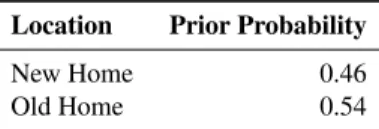
New Home. This characteristic specifies if the borrower is pur-chasing a newly built property or a previously occupied prop-erty. The prior probabilities are displayed in Table 13. The data is obtained from DEHLG housing statistics (DofE, 2008) (Ownership status of borrowerstab). The characteristic is not actually used during the labelling process (see Section 4.2). It is only used in the data generation process as part of the
statis-Table 12: List of prior probabilities for Location characteristic
Location Prior Probability
Dublin 0.32 Cork 0.15 Galway 0.07 Limerick 0.04 Waterford 0.03 Other 0.39
tics provided by the DEHLG (DofE, 2008) are based on this characteristic.
Table 13: List of prior probabilities for New Home characteristic
Location Prior Probability
New Home 0.46
Old Home 0.54
Loan Value Group. This characteristic describes the principal of the loan. The nine categories and prior probabilities used by Loan Value Group are similar to those used by DEHLG hous-ing statistics (DofE, 2008) (Range of loans paidtab), the dif-ference being we further sub-divided the final two categories resulting in two additional categories. The prior probabilities, conditional on the Location; New Home; and FTB characteris-tics, are specified in Table 14. The precise loan value for each borrower is a randomly generated value between the category start and end values. For simplicity we restrict the maximum loan value to 900,000. We employ the assumption that any val-ues greater than this amount require an additional assessment of creditworthiness in the form of a personal interview with a member of the bank’s staff.
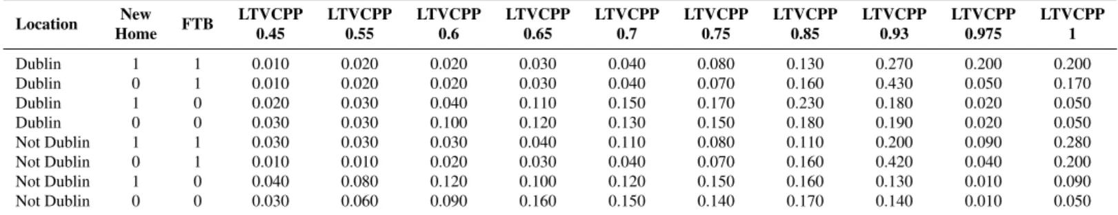
Loan-to-Value (LTV). This characteristic expresses the ratio of the loan value to the market value of the asset. Based on data from DEHLG housing statistics (DofE, 2008) (Ranges of loans to valuetab) we use 10 categories ranging from 45% to 100%, as per Table 15. We subdivide one of the original categories (“Up to 70%”) into five seperate categories as its conditional prior probability was quite large (52% in some cases). The prior probabilities of the LTV categories are conditional on the Lo-cation, New Home, and FTB characteristics.
Loan Term. The duration of the loan in years is captured by the Loan Term characteristic. The data is based on DEHLG housing statistics (DofE, 2008) (Ranges of loan termstab). Five categories are employed: (i) 20 years; (ii) 25 years; (iii) 30 years; (iv) 35 years; and (v) 40 years. The prior probabilities are conditional on Location and FTB. We have also added Age Group as a conditional prior probability to ensure the values are realistic, as per Table 16.
House Value. This characteristic represents the market value of the asset. It is calculated as Loan Value divided by Loan-To-Value. House Value is generated as a continuous value that is then converted in a categorical value. The categorical val-ues are based on categories used by DEHLG housing statis-tics (DofE, 2008) (Range of house pricestab), with one of the categories (300,001 to 400,000) subdivided into two separate categories (300,001 to 350,000and350,001 to 400,000). The categories used are (i) 0 to 150,000; (ii) 150,001 to 200,000; (iii) 200,001 to 250,000; (iv) 250,001 to 300,000; (v) 300,001 to 350,000; (vi) 350,001 to 400,000; (vii) 400,001 to 500,000; (viii) 500,001+.
Loan Rate. This characteristic represents the interest rate paid by the borrower on the loan. For the simplicity of the monthly mortgage repayments we do not consider interest only loans. The breakdown between Fixed and Variable interest rate loans is provided by DEHLG housing statistics (DofE, 2008) (Fixed
& var interest rate loans tab). We further subdivide these two categories into 6 categories: (i) Fixed - Over 5 years; (ii) Tracker Type 1; (iii) Tracker Type 2; (iv) Standard Variable; (v) Up to 1 year fixed; and (vi) Fixed - 3 to 5 years, as per Table 17
Table 17: Loan Rate prior probabilities
Loan Rate Description Interest Rate Prior Probability
Fixed−Over 5 years 0.0535 0.450
Tracker Type 1 0.0150 0.150
Tracker Type 2 0.0250 0.100
Standard Variable 0.0350 0.150
Up to 1 year fixed 0.0450 0.090
Fixed−3 to 5 years 0.0500 0.060
Monthly-Repayments-to-Income (MRTI). This is a continuous characteristic which expresses monthly mortgage repayments as a percentage of monthly income.
All of the above conditional prior probabilities are user de-fined parameters, the values we have specified attempt to repli-cate the Irish mortgage market in 2007. Another user defined parameter is the population size of the data to be generated, the default value is 2,000 instances.
4.2. Label Application
For each instance generated, the constituent characteristics are assigned a risk score which are then aggregated into an overall risk score for the instance. The higher the risk score, the greater the likelihood of default. Coded business intelli-gence rules are used to determine the risk score of a charac-teristic value. These business intelligence rules have been de-vised as a product of extensive consultations with a credit risk scorecard expert. Additional information was also provided in the Moody’s report (Moodys, 2010) on Irish defaulters and a Central Bank of Ireland technical report (McCarthy and Mc-Quinn, 2010). By presenting a realistic assessment of credit
Table 14: Loan Value Group conditional prior probabilities (LVGCPP) for each Loan Value Group category. Loan Value Group values are displayed in ’000. The
CPP of each row should sum to 1. Certain locations have been combined, Wtf=Waterford.
Location FTB New LVGCCP LVGCCP LVGCCP LVGCCP LVGCCP LVGCCP LVGCCP LVGCCP LVGCCP Home 50 - 100 100 - 150 150 - 200 200 - 250 250 - 300 300 - 350 350 - 400 400 - 450 450 - 900 Dublin 1 1 0.01 0.03 0.13 0.30 0.27 0.12 0.07 0.06 0.01 Dublin 0 1 0.02 0.04 0.10 0.15 0.18 0.13 0.14 0.16 0.08 Dublin 1 0 0.01 0.03 0.06 0.13 0.25 0.28 0.10 0.11 0.03 Dublin 0 0 0.08 0.05 0.08 0.12 0.15 0.13 0.12 0.15 0.12 Cork\Galway 1 1 0.06 0.14 0.31 0.24 0.17 0.07 0.01 0.01 0.00 Cork\Galway 0 1 0.08 0.13 0.21 0.22 0.15 0.11 0.04 0.05 0.02 Cork\Galway 1 0 0.04 0.08 0.18 0.27 0.23 0.12 0.05 0.02 0.00 Cork\Galway 0 0 0.11 0.13 0.19 0.17 0.11 0.16 0.09 0.02 0.02 Limerick\Wtf 1 1 0.06 0.16 0.34 0.25 0.13 0.05 0.01 0.01 0.00 Limerick\Wtf 0 1 0.10 0.18 0.23 0.23 0.15 0.05 0.04 0.02 0.01 Limerick\Wtf 1 0 0.06 0.12 0.20 0.25 0.22 0.11 0.02 0.01 0.01 Limerick\Wtf 0 0 0.23 0.19 0.22 0.18 0.11 0.02 0.02 0.02 0.02 Other 1 1 0.05 0.15 0.36 0.28 0.11 0.04 0.01 0.01 0.00 Other 0 1 0.10 0.11 0.24 0.17 0.18 0.08 0.05 0.05 0.03 Other 1 0 0.05 0.14 0.24 0.28 0.18 0.08 0.02 0.01 0.01 Other 0 0 0.16 0.20 0.21 0.17 0.14 0.04 0.03 0.03 0.02
Table 15: LTV conditional prior probabilities (LTVCPP) for each LTV category. The CPP of each row should sum to 1.
Location New FTB LTVCPP LTVCPP LTVCPP LTVCPP LTVCPP LTVCPP LTVCPP LTVCPP LTVCPP LTVCPP Home 0.45 0.55 0.6 0.65 0.7 0.75 0.85 0.93 0.975 1 Dublin 1 1 0.010 0.020 0.020 0.030 0.040 0.080 0.130 0.270 0.200 0.200 Dublin 0 1 0.010 0.020 0.020 0.030 0.040 0.070 0.160 0.430 0.050 0.170 Dublin 1 0 0.020 0.030 0.040 0.110 0.150 0.170 0.230 0.180 0.020 0.050 Dublin 0 0 0.030 0.030 0.100 0.120 0.130 0.150 0.180 0.190 0.020 0.050 Not Dublin 1 1 0.030 0.030 0.030 0.040 0.110 0.080 0.110 0.200 0.090 0.280 Not Dublin 0 1 0.010 0.010 0.020 0.030 0.040 0.070 0.160 0.420 0.040 0.200 Not Dublin 1 0 0.040 0.080 0.120 0.100 0.120 0.150 0.160 0.130 0.010 0.090 Not Dublin 0 0 0.030 0.060 0.090 0.160 0.150 0.140 0.170 0.140 0.010 0.050
Table 16: Loan Term conditional prior probabilities (LTCPP) for each Loan Term category. The CPP of each row should add to 1.
Location FTB Age LTCPP LTCPP LTCPP LTCPP LTCPP 20 25 30 35 40 Dublin 1 18 - 25 0.010 0.030 0.080 0.800 0.080 Dublin 1 26 - 30 0.020 0.060 0.160 0.720 0.040 Dublin 1 31 - 35 0.020 0.060 0.160 0.720 0.040 Dublin 1 36 - 40 0.020 0.060 0.160 0.720 0.040 Dublin 1 41 - 45 0.100 0.730 0.120 0.050 0.000 Dublin 1 46 - 55 0.120 0.750 0.080 0.050 0.000 Dublin 0 18 - 25 0.120 0.140 0.210 0.480 0.050 Dublin 0 26 - 30 0.230 0.280 0.220 0.240 0.030 Dublin 0 31 - 35 0.220 0.320 0.190 0.240 0.030 Dublin 0 36 - 40 0.220 0.320 0.190 0.240 0.030 Dublin 0 41 - 45 0.220 0.320 0.250 0.200 0.010 Dublin 0 46 - 55 0.220 0.320 0.240 0.220 0.000 Not Dublin 1 18 - 25 0.030 0.050 0.170 0.680 0.070 Not Dublin 1 26 - 30 0.050 0.090 0.180 0.620 0.060 Not Dublin 1 31 - 35 0.060 0.110 0.200 0.590 0.040 Not Dublin 1 36 - 40 0.060 0.110 0.200 0.590 0.040 Not Dublin 1 41 - 45 0.140 0.290 0.300 0.250 0.020 Not Dublin 1 46 - 55 0.340 0.390 0.140 0.130 0.000 Not Dublin 0 18 - 25 0.060 0.090 0.120 0.410 0.320 Not Dublin 0 26 - 30 0.140 0.150 0.250 0.320 0.140 Not Dublin 0 31 - 35 0.220 0.330 0.240 0.190 0.020 Not Dublin 0 36 - 40 0.220 0.330 0.240 0.190 0.020 Not Dublin 0 41 - 45 0.130 0.460 0.290 0.100 0.020 Not Dublin 0 46 - 55 0.140 0.680 0.100 0.080 0.000
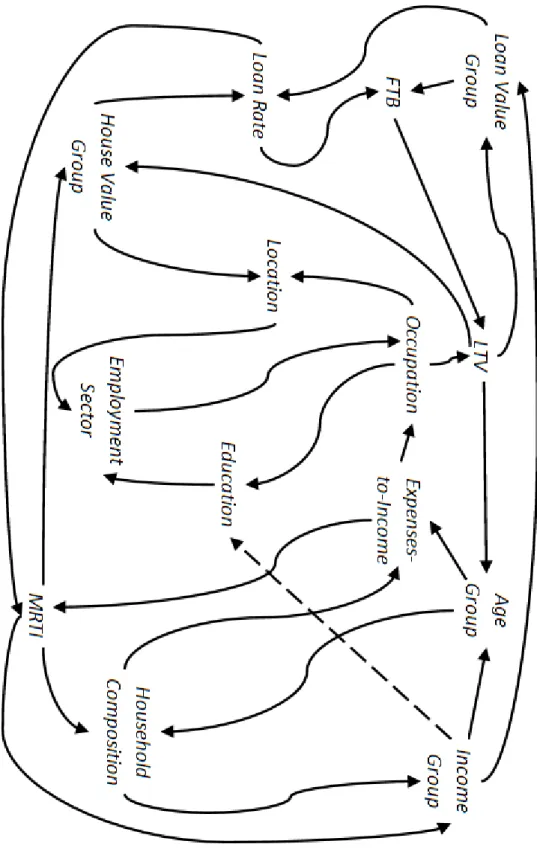
risk, the business intelligence rules generate non-linear distri-butions based on interactions between the characteristics. Inter-actions occur when different predictive patterns exist for diff er-ent subgroups within the population (Anderson, 2007). Without any such attempt to define the interactions between the charac-teristics, the generated dataset would otherwise present a trivial classification task. The rest of this section outlines the business intelligence rules and specified interactions used to generate la-bels. The characteristics with which a specific characteristic has an interaction are listed in parentheses. Figure 1 also illustrates the interactions between the characteristics. After the credit risk score of an instance is calculated a user defined noise random Gaussian noise can be added (subtracted) to (from) this value. Based on a user specified bad rate, a cut-offscore is identified whereby those instances with a value equal to or greater than the cut-offscore are labelled as defaulters (Bads) and those less than the cut-offscore are labelled as repayers (Goods). In order to complicate the classification task and to mimic real-world unpredictability, a user-defined swap rate can then be applied, whereby a percentage of repayers are randomly selected and their labels are reassigned as defaulter.
MRTI (Loan Rate, Expenses-to-Income). In general, when granting credit, a safe figure for a borrower’s MRTI should be no more than 33%. The Loan Rate is one of the main vari-ables used when calculating the monthly mortgage repayment amount. The Expenses-to-Income ratio and MRTI should both be able to provide a clear indication of a borrower’s overall expenditure. A borrower with a relatively high MRTI (33% -38%) may initially appear a risky prospect. However, this risk is reduced somewhat if their Expenses-to-Income ratio is low and their Loan Rate is fixed (i.e. the loan repayments are not subject to any variability for the foreseeable future). For scoring purposes the MRTI is split into 5 equal sized monotonically-ordered quantiles. However, the size of the quantiles may differ after unrealistic values have been removed. After the labelling process has been completed the MRTI ratios are stored as con-tinuous values.
Loan Value Group (Income Group, LTV). The business intelli-gence rules are coded under the assumption that the higher the loan value the greater the risk of default, as per Moody’s report (Moodys, 2010). However, this risk may be offset by a high level of Income or a low LTV. A high level of income indicates the borrower’s ability to service a large loan. A low LTV sug-gests that the borrower has already invested too much in the loan to simply walk away.
Employment Sector (Location, Education). The Employment Sector represents, to some degree, the borrower’s job security and earnings. For example, a borrower employed by the gov-ernment is considered less risky than a construction worker. Lo-cation is included as it relates to the availability of commensu-rate employment opportunities within the same locale, i.e. the size of the jobs market. For example, a borrower working in the Industry sector in a sparsely populated area, such as Wa-terford, is considered a risk as there are fewer opportunities to
find alternative employment in the same Industry as compared to a larger and more industrially active centre such as Dublin. Education attempts to capture the skill set of the borrower. The business intelligence rules operate under the assumption that the more educated the borrower, the easier to move between employment sectors.
Occupation (Employment Sector, Expenses-to-Income). Based on (Moodys, 2010) we assign self-employed borrowers as the most likely to default. Borrowers belonging to the Manager, Administrator, and Professional (MAP) Employment Sector category are considered the least likely to default - due to their importance to an organisation as well as the demand for their skills and experience. The Employment Sector characteristic helps determine the demand for a particular Occupation. For example, a bureaucratic sector such as Health would have a higher demand for MAP employees than a sector such as Hos-pitality. By using a borrower’s Occupation along with their Expenses-To-Income the business intelligence rules attempt to capture the borrower’s social status and the cost to maintain it.
Location (House Value Group, Occupation). The ability to sell or rent a house can reduce the likelihood of default. Dublin and Cork are the main rental markets in Ireland and as such represent a lower risk of default. For the next three locations: Galway, Limerick, and Waterford the risk of default increases proportionally as the size of the rental market decreases. Other is considered the riskiest location of the six as it represents the least densely populated areas. House Value is used to indicate that for some locations (i.e. Dublin) houses are over valued, as per 2007. The more overpriced a home, the greater the risk of default on account of the negative equity that may arise when house prices return to their longterm average. Occupation, in the context of Location, indicates that the level of demand for a borrower’s expertise and experience varies from location to location. Typically, a populous location indicates a large and diverse jobs market.
Income Group (Household Composition, MRTI). A borrower with a high level of income is considered less likely to de-fault. Household Composition is used to indicate the level of income required to maintain the household. Ordinarily, 2 Adults, 1+child<18is considered to have a lower chance of default compared to2 Adults, No childas they are more likely to have stronger community ties through family involvement. The MRTI indicates the amount of income required to service the loan. For example, a borrower on a high income with a high MRTI is considered a greater default risk than a borrower on a mid-level income with a low MRTI.
Household Composition (Age Group, MRTI). The Household Composition affects the risk of default with regard to earnings power, and the priorities of household members. A single per-son household represents a higher risk of defaulting compared to the 2 Adults, No childcategory as the impact of a loss of income to the couple may be less severe. From a Household Composition perspective, the Age Group represents the type of
Figure 1: Interactions between the dataset characteristics
dependencies the borrower may have. For example a young2 Adults, 1+child<18will likely have to pay for school/doctor fees. The MRTI indicates the burden the household is under to pay bills. A household with no dependents and a high MRTI is less risky than a household with children and a high MRTI, as the welfare of the children will come first.
Age Group (Income Group, LTV). Younger borrowers repre-sent a greater risk of default than older borrowers. However, older borrowers still present a risk due to illness and death. In-come Group, in the context of Age Group, indicates the present and future earning potential of a borrower. A young person on a high income can be interpreted as a skilled individual and therefore low risk. As the LTV reflects the amount of savings a borrower has contributed to the loan, the Age Group indicates how long the borrower has to rebuild their savings.
FTB (Loan Value Group, Loan Rate). Due to a lack of expe-rience, a First-Time-Buyer is considered more likely to default on a loan than a non-FTB. A high Loan Value Group places greater pressure on the borrower to manage their finances. The Loan Rate indicates the borrower’s financial aptitude at select-ing an appropriate loan product. For example a FTB with a fixed rate is considered risk averse compared to a FTB with a variable rate.
Education (Income Group, Occupation). A borrower’s level of formal Education impacts the risk of default. The more edu-cated an individual, the more financially astute they are likely to be. A high level of education also improves job prospects. Income Group affects Education in terms of the ability to afford training courses and improve skill levels. A borrower’s Occu-pation indicates their ability to apply their education in terms of over-achievement or under-achievement, i.e. a measure of their drive to overcome obstacles.
Loan Rate (House Value Group, Loan Value Group). There are three different Loan Rates: (i) Fixed rate loans which are con-sidered the least risky; (ii) Tracker rate loans which are slightly more risky; and (iii) Variable rate loans which are considered the riskiest of the three. In terms of the Loan Rate, the Loan Value Group affects risk based on the fact that the size of the repayments increase with the size of the Loan Value. In gen-eral, interest rates can affect the availability of capital and de-mand for investment. As interest rates were at a historically low level in 2007, the business intelligence rules are based on the assumption that interest rates will rise. As interest rates rise, a more expensive house will be harder to sell. Rising interest rates may cause the house value to decline, and increase the possibility of negative equity.
Expenses-To-Income (Household Composition, Age Group).
The greater the Expenses-to-Income ratio the higher the risk of default. Household Composition is a strong indicator of how much money the borrower needs to spend on groceries, utility bills, fees etc. The Age group helps identify the level and the necessity of the expenses. For example, a young single person would be expected to have a high Expenses-to-Income ratio but
much of it may involve expenditure on items such as holidays or concert tickets. During the labelling process the Expenses-to-Income ratios are split into 5 equal sized monotonically-ordered quantiles. However, the size of the quantiles may differ after un-realistic values have been removed. After the labelling process has been completed the Expenses-to-Income ratios are stored as continuous values.
LTV (First-Time-Buyer, Occupation). When assessing LTV for the risk of default the business intelligence rules consider the size of the deposit fronted by the borrower. In the event of a de-fault, a high LTV indicates the borrower will suffer less of a loss compared to someone who has already invested a large amount of savings. In improving market conditions a FTB can expect to sell their house at a profit. A non-FTB with a high LTV may indicate poor financial management, or over stretching when trading up. Based on reputation, higher ranked Occupations are able to receive a higher LTV and should not be penalised as such.
House Value Group (LTV, MRTI). The greater the house value the less likely the borrower will default. Other factors to consider when assessing risk based on the house value is the size of the deposit paid by the borrower and the amount of income required to service the loan.
This section has described the methodology used to gen-erate data and the process used to label the data. The risk score of a characteristic value is determined by coded business intelligence rules that have been devised based on consultations with a credit risk expert. The characteristic risk scores for an instance are then aggregated together to give a credit risk score for the instance. Based on a specified default rate, a cut-off score is determined whereby a percentage of the highest credit risk scores are assigned as defaulters. The business intelligence rules help to complicate the classification task by specifying non-linear interactions between the various characteristics.
5. Experimental Results
This section discusses the properties of a generated artificial dataset and illustrates the realistic nature of the artificial data. Using the conditional prior probabilities previously defined a dataset containing 3,000 instances is generated. An initial de-fault rate of 3% is specified, along with a swap rate of 0.5% (i.e. the percentage of instances originally labelled Good but are re-assigned as Bad). This is an accurate approximation of the Irish default rate in 2007. The maximum affordability1 is defined as 10, and the maximum MRTI is set at 90%. As a result, 119 (3.97%) instances are discarded as they exceed at least one of these values.
After the removal of unrealistic values, the dataset consists of 101 (3.51%) defaulters and 2780 (96.49%) repayers. As a starting point, a comparison between the artificial data and real-world data reported in Moody’s (Moodys, 2010) is detailed in
Table 18. This table indicates that the conditional prior proba-bilities of three of the characteristics (House Value Group, Loan Value Group, and LTV as it is used to calculate House Value) are reasonably accurate.
Table 18: Comparison of generated artificial data with real-world. House Value and Loan Value in ’000.
Characteristic Category Artificial Moody’s
Data
House Value Group <200 24% 17%
200 - 400 52% 51%
400 - 600 18% 18%
600 - 800 4% 6%
800 - 1,000 1% 3%
>1,000 1% 5%
Loan Value Group <200 40% 38%
200 - 400 52% 49%
400 - 600 6% 8%
600 - 800 1% 2%
800 - 1,000 1% 1%
>1,000 0% 2%
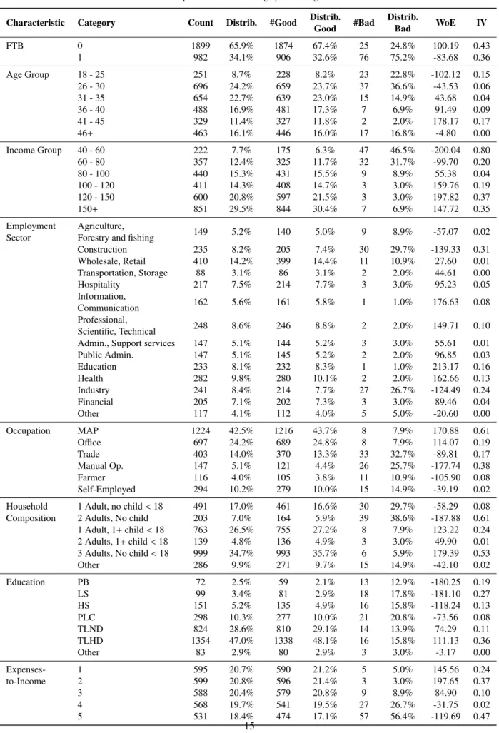
Tables 19 and 20 describe the distribution of the data for the borrower and loan demographics, respectively. Also reported are the weights of evidence (WoE) and information value (IV) for each of the categories. The WoE measures the predictive power of each category. The calculated value of the WoE is dependent on a binary outcome (i.e. good or bad). The WoE of a category is calculated as the logrithm of the ratio of the proportion of goods to the proportion of bads. In keeping with common practice the values have been multiplied by 100 in or-der to make the figures more readable. A large negative WoE value corresponds to a high risk of default, while a high positive value corresponds to a low risk.
Based on Table 19, the standard borrower demographics of a defaulter are likely to be: (i) a FTB (as per 75.2% of default-ers); (ii) less than 31 years of age (as per 59.4% of defaultdefault-ers); (iii) earn less than 80,000 (as per 78.2% of defaulters); (iv) is employed in the Construction or Industry sectors (as per 56.4% of defaulters); (v) as an Occupation they are classed Farmer or Self-Employed (as per 36.6% of defaulters); (vi) they are likely to be part of either a 2 Adults, No child household or 1 Adult, no child<18 household (as per 68.3% of defaulters); (vii) non-college educated, i.e. PB, LS, HS, or PLC (as per 67.3% of defaulters); and (vii) have an Expenses-to-Income ratio in the highest two quantiles (as per 83.1% of defaulters).
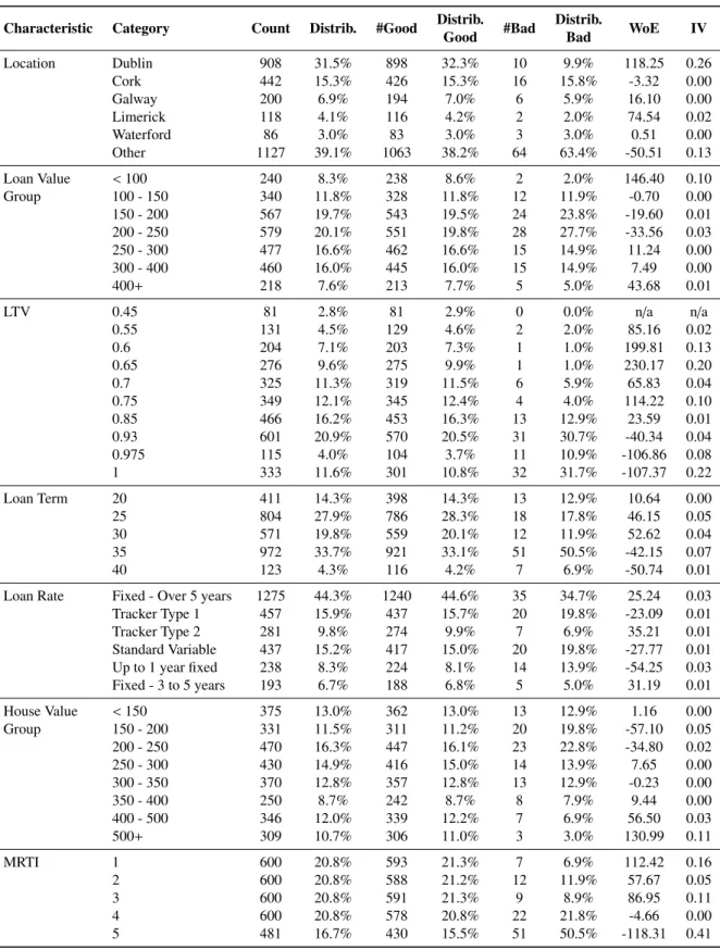
Based on Table 20, the standard loan demographics of a de-faulter are likely to: (i) live in Other (as per 63.4% of default-ers); (ii) have a loan value of between 100,000 and 250,000 (as per 63.4% of defaulters); (iii) have a LTV of 0.93 or greater (as per 73.3% of defaulters); (iv) have a loan term of at least 35 years (as per 57.4% of defaulters); (v) have a Loan Rate based on either a standard variable or up-to-one-year fixed (as per 33.7% of defaulters); (vi) a house value of between 150,000 and 250,000 (as per 42.6% of defaulters); and (vii) have an MRTI ratio in the top two quantiles (as per 72.3% of defaulters).
The IV is used to assess the overall predictive strength of a characteristic. Table 21 provides the IV score for each charac-teristic. The characteristics are ordered based on their predic-tive strength with Income Group, Household Composition, and Occupation as the most predictive characteristics based on IV. Loan Rate, Loan Value Group, and Loan Term are deemed the weakest, this can be attributed in part to the removal of unreal-istic values based on high affordability caused by large loan val-ues. One would normally expect LTV and MRTI to be ranked higher, but again, as the more severe and unrealistic values are removed the predictive strength of the characteristics is weak-ened. Only 2.67% of the instances have an MRTI value greater then 33%.
Any characteristic with an IV score less than 0.02 should be rejected. An IV score above 0.3 and the characteristic is con-sidered a strong predictor, and anything above 0.5 indicates the characteristic is over-predicting. As the described data is so im-balanced and artificially generated it is unsurprising that the IV scores are so large.
As an alternative approach, the user could generate 20,000 instances using the same default rate and swap rate. As before, unrealistic instances would be removed using a maximum af-fordability and MRTI rate. The user could then undersample the majority class to produce a balanced dataset.
Table 21: Information Value
Characteristic IV Income Group 1.94 Household Comp. 1.49 Occupation 1.45 Expenses-to-Income 1.20 Employment Sect 1.19 Education 1.15 LTV 0.84 FTB 0.78 MRTI 0.74 Age Group 0.51 Location 0.41
House Value Group 0.21
Loan Term 0.18
Loan Value Group 0.15
Loan Rate 0.10
6. Case Study: Population Drift
The following section examines the effects of population drift on the predictive performance of a classification model. This exercise also demonstrates the usefulness of our artificial data generation framework through the creation of datasets whose distributions gradually change over time.
6.1. Population Drift Background
Credit risk scorecards have a limited lifespan, and often their performance degrades over time. During scorecard construc-tion samples drawn from data representative of the current pop-ulation will rarely have the same distribution as those drawn
Table 19: Description of borrower demographics from generated dataset
Characteristic Category Count Distrib. #Good Distrib. #Bad Distrib. WoE IV
Good Bad FTB 0 1899 65.9% 1874 67.4% 25 24.8% 100.19 0.43 1 982 34.1% 906 32.6% 76 75.2% -83.68 0.36 Age Group 18 - 25 251 8.7% 228 8.2% 23 22.8% -102.12 0.15 26 - 30 696 24.2% 659 23.7% 37 36.6% -43.53 0.06 31 - 35 654 22.7% 639 23.0% 15 14.9% 43.68 0.04 36 - 40 488 16.9% 481 17.3% 7 6.9% 91.49 0.09 41 - 45 329 11.4% 327 11.8% 2 2.0% 178.17 0.17 46+ 463 16.1% 446 16.0% 17 16.8% -4.80 0.00 Income Group 40 - 60 222 7.7% 175 6.3% 47 46.5% -200.04 0.80 60 - 80 357 12.4% 325 11.7% 32 31.7% -99.70 0.20 80 - 100 440 15.3% 431 15.5% 9 8.9% 55.38 0.04 100 - 120 411 14.3% 408 14.7% 3 3.0% 159.76 0.19 120 - 150 600 20.8% 597 21.5% 3 3.0% 197.82 0.37 150+ 851 29.5% 844 30.4% 7 6.9% 147.72 0.35 Employment Agriculture, 149 5.2% 140 5.0% 9 8.9% -57.07 0.02
Sector Forestry and fishing
Construction 235 8.2% 205 7.4% 30 29.7% -139.33 0.31 Wholesale, Retail 410 14.2% 399 14.4% 11 10.9% 27.60 0.01 Transportation, Storage 88 3.1% 86 3.1% 2 2.0% 44.61 0.00 Hospitality 217 7.5% 214 7.7% 3 3.0% 95.23 0.05 Information, 162 5.6% 161 5.8% 1 1.0% 176.63 0.08 Communication Professional, 248 8.6% 246 8.8% 2 2.0% 149.71 0.10 Scientific, Technical
Admin., Support services 147 5.1% 144 5.2% 3 3.0% 55.61 0.01
Public Admin. 147 5.1% 145 5.2% 2 2.0% 96.85 0.03 Education 233 8.1% 232 8.3% 1 1.0% 213.17 0.16 Health 282 9.8% 280 10.1% 2 2.0% 162.66 0.13 Industry 241 8.4% 214 7.7% 27 26.7% -124.49 0.24 Financial 205 7.1% 202 7.3% 3 3.0% 89.46 0.04 Other 117 4.1% 112 4.0% 5 5.0% -20.60 0.00 Occupation MAP 1224 42.5% 1216 43.7% 8 7.9% 170.88 0.61 Office 697 24.2% 689 24.8% 8 7.9% 114.07 0.19 Trade 403 14.0% 370 13.3% 33 32.7% -89.81 0.17 Manual Op. 147 5.1% 121 4.4% 26 25.7% -177.74 0.38 Farmer 116 4.0% 105 3.8% 11 10.9% -105.90 0.08 Self-Employed 294 10.2% 279 10.0% 15 14.9% -39.19 0.02
Household 1 Adult, no child<18 491 17.0% 461 16.6% 30 29.7% -58.29 0.08
Composition 2 Adults, No child 203 7.0% 164 5.9% 39 38.6% -187.88 0.61
1 Adult, 1+child<18 763 26.5% 755 27.2% 8 7.9% 123.22 0.24 2 Adults, 1+child<18 139 4.8% 136 4.9% 3 3.0% 49.90 0.01 3 Adults, No child<18 999 34.7% 993 35.7% 6 5.9% 179.39 0.53 Other 286 9.9% 271 9.7% 15 14.9% -42.10 0.02 Education PB 72 2.5% 59 2.1% 13 12.9% -180.25 0.19 LS 99 3.4% 81 2.9% 18 17.8% -181.10 0.27 HS 151 5.2% 135 4.9% 16 15.8% -118.24 0.13 PLC 298 10.3% 277 10.0% 21 20.8% -73.56 0.08 TLND 824 28.6% 810 29.1% 14 13.9% 74.29 0.11 TLHD 1354 47.0% 1338 48.1% 16 15.8% 111.13 0.36 Other 83 2.9% 80 2.9% 3 3.0% -3.17 0.00 Expenses- 1 595 20.7% 590 21.2% 5 5.0% 145.56 0.24 to-Income 2 599 20.8% 596 21.4% 3 3.0% 197.65 0.37 3 588 20.4% 579 20.8% 9 8.9% 84.90 0.10 4 568 19.7% 541 19.5% 27 26.7% -31.75 0.02 5 531 18.4% 474 17.1% 57 56.4% -119.69 0.47
Table 20: Description of loan demographics from generated dataset
Characteristic Category Count Distrib. #Good Distrib. #Bad Distrib. WoE IV
Good Bad Location Dublin 908 31.5% 898 32.3% 10 9.9% 118.25 0.26 Cork 442 15.3% 426 15.3% 16 15.8% -3.32 0.00 Galway 200 6.9% 194 7.0% 6 5.9% 16.10 0.00 Limerick 118 4.1% 116 4.2% 2 2.0% 74.54 0.02 Waterford 86 3.0% 83 3.0% 3 3.0% 0.51 0.00 Other 1127 39.1% 1063 38.2% 64 63.4% -50.51 0.13 Loan Value <100 240 8.3% 238 8.6% 2 2.0% 146.40 0.10 Group 100 - 150 340 11.8% 328 11.8% 12 11.9% -0.70 0.00 150 - 200 567 19.7% 543 19.5% 24 23.8% -19.60 0.01 200 - 250 579 20.1% 551 19.8% 28 27.7% -33.56 0.03 250 - 300 477 16.6% 462 16.6% 15 14.9% 11.24 0.00 300 - 400 460 16.0% 445 16.0% 15 14.9% 7.49 0.00 400+ 218 7.6% 213 7.7% 5 5.0% 43.68 0.01 LTV 0.45 81 2.8% 81 2.9% 0 0.0% n/a n/a 0.55 131 4.5% 129 4.6% 2 2.0% 85.16 0.02 0.6 204 7.1% 203 7.3% 1 1.0% 199.81 0.13 0.65 276 9.6% 275 9.9% 1 1.0% 230.17 0.20 0.7 325 11.3% 319 11.5% 6 5.9% 65.83 0.04 0.75 349 12.1% 345 12.4% 4 4.0% 114.22 0.10 0.85 466 16.2% 453 16.3% 13 12.9% 23.59 0.01 0.93 601 20.9% 570 20.5% 31 30.7% -40.34 0.04 0.975 115 4.0% 104 3.7% 11 10.9% -106.86 0.08 1 333 11.6% 301 10.8% 32 31.7% -107.37 0.22 Loan Term 20 411 14.3% 398 14.3% 13 12.9% 10.64 0.00 25 804 27.9% 786 28.3% 18 17.8% 46.15 0.05 30 571 19.8% 559 20.1% 12 11.9% 52.62 0.04 35 972 33.7% 921 33.1% 51 50.5% -42.15 0.07 40 123 4.3% 116 4.2% 7 6.9% -50.74 0.01
Loan Rate Fixed - Over 5 years 1275 44.3% 1240 44.6% 35 34.7% 25.24 0.03
Tracker Type 1 457 15.9% 437 15.7% 20 19.8% -23.09 0.01 Tracker Type 2 281 9.8% 274 9.9% 7 6.9% 35.21 0.01 Standard Variable 437 15.2% 417 15.0% 20 19.8% -27.77 0.01 Up to 1 year fixed 238 8.3% 224 8.1% 14 13.9% -54.25 0.03 Fixed - 3 to 5 years 193 6.7% 188 6.8% 5 5.0% 31.19 0.01 House Value <150 375 13.0% 362 13.0% 13 12.9% 1.16 0.00 Group 150 - 200 331 11.5% 311 11.2% 20 19.8% -57.10 0.05 200 - 250 470 16.3% 447 16.1% 23 22.8% -34.80 0.02 250 - 300 430 14.9% 416 15.0% 14 13.9% 7.65 0.00 300 - 350 370 12.8% 357 12.8% 13 12.9% -0.23 0.00 350 - 400 250 8.7% 242 8.7% 8 7.9% 9.44 0.00 400 - 500 346 12.0% 339 12.2% 7 6.9% 56.50 0.03 500+ 309 10.7% 306 11.0% 3 3.0% 130.99 0.11 MRTI 1 600 20.8% 593 21.3% 7 6.9% 112.42 0.16 2 600 20.8% 588 21.2% 12 11.9% 57.67 0.05 3 600 20.8% 591 21.3% 9 8.9% 86.95 0.11 4 600 20.8% 578 20.8% 22 21.8% -4.66 0.00 5 481 16.7% 430 15.5% 51 50.5% -118.31 0.41