Financial
Institutions
Center
Consumer Response to Changes in
Credit Supply: Evidence from Credit
Card Data
by
David Gross Nicholas Souleles 01-10
The Wharton Financial Institutions Center
The Wharton Financial Institutions Center provides a multi-disciplinary research approach to the problems and opportunities facing the financial services industry in its search for competitive excellence. The Center's research focuses on the issues related to managing risk at the firm level as well as ways to improve productivity and performance.
The Center fosters the development of a community of faculty, visiting scholars and Ph.D. candidates whose research interests complement and support the mission of the Center. The Center works closely with industry executives and practitioners to ensure that its research is informed by the operating realities and competitive demands facing industry participants as they pursue competitive excellence.
Copies of the working papers summarized here are available from the Center. If you would like to learn more about the Center or become a member of our research community, please let us know of your interest.
Franklin Allen Richard J. Herring
Co-Director Co-Director
The Working Paper Series is made possible by a generous grant from the Alfred P. Sloan Foundation
Consumer Response to Changes in Credit Supply:
Evidence from Credit Card Data
†David B. Gross Nicholas S. Souleles Graduate School of Business Finance Department University of Chicago The Wharton School
University of Pennsylvania
this draft: February 4, 2000
Abstract
This paper utilizes a unique new data set on credit card accounts to analyze how people respond to changes in credit supply. The data consist of a panel of several hundred thousand individual credit card accounts followed monthly for 24-36 months, from several different card issuers, with associated credit bureau data. We estimate the dynamic effects of changes in the credit limit and in interest rates, and consider the ability of different models of consumption and saving to rationalize these effects.
We find that increases in credit limits generate an immediate and significant rise in debt. This response is sharpest for people starting near their limit, providing evidence that liquidity constraints are binding. However, even people starting well below their limit significantly respond. We show this result is consistent with conventional models of precautionary savings. Nonetheless there are other results that conventional models cannot easily explain, such as the fact that many credit card borrowers simultaneously hold other low yielding assets. Unlike most other studies, we also find strong effects from changes in account-specific interest rates. Debt is particularly sensitive to large declines in interest rates, which can explain the widespread use of teaser rates. The long-run elasticity of debt to the interest rate is about -1.3. Less than half of this elasticity represents balance-switching across cards, with most reflecting net changes in total borrowing. Overall, the results imply that the consumer plays a potentially important role in the transmission of monetary policy and other credit shocks.
Keywords: liquidity constraints, precautionary saving, intertemporal elasticity of substitution; consumer credit, credit cards; monetary policy, credit supply, credit channel.
JEL classification: E21, E51, G21
†
We would like to thank Larry Ausubel, Kathleen Johnson, Anil Kashyap, Tony Santomero, and seminar participants at the New York Fed, ASSA meetings, Carnegie-Mellon, Columbia, the NBER Summer Institute, and various workshops at the University of Chicago GSB and The Wharton School. We are grateful to the Wharton Financial Institutions Center and several credit card issuers for numerous discussions and assistance in acquiring the data. All remaining errors are our own.
Consumer Response to Changes in Credit Supply:
Evidence from Credit Card Data
Abstract
This paper utilizes a unique new data set on credit card accounts to analyze how people respond to changes in credit supply. The data consist of a panel of several hundred thousand individual credit card accounts followed monthly for 24-36 months, from several different card issuers, with associated credit bureau data. We estimate the dynamic effects of changes in the credit limit and in interest rates, and consider the ability of different models of consumption and saving to rationalize these effects.
We find that increases in credit limits generate an immediate and significant rise in debt. This response is sharpest for people starting near their limit, providing evidence that liquidity constraints are binding. However, even people starting well below their limit significantly respond. We show this result is consistent with conventional models of precautionary savings. Nonetheless there are other results that conventional models cannot easily explain, such as the fact that many credit card borrowers simultaneously hold other low yielding assets. Unlike most other studies, we also find strong effects from changes in account-specific interest rates. Debt is particularly sensitive to large declines in interest rates, which can explain the widespread use of teaser rates. The long-run elasticity of debt to the interest rate is about -1.3. Less than half of this elasticity represents balance-switching across cards, with most reflecting net changes in total borrowing. Overall, the results imply that the consumer plays a potentially important role in the transmission of monetary policy and other credit shocks.
Keywords: liquidity constraints, precautionary saving, intertemporal elasticity of substitution; consumer credit, credit cards; monetary policy, credit supply, credit channel.
1. Introduction
Empirical studies of the consumer have found it difficult to identify the effects of changes in credit supply. For instance, most studies find little sensitivity of saving to interest rates and there is still no agreement about whether liquidity constraints and precautionary motives are in practice important (Browning and Lusardi, 1996). Studies of the credit channel and monetary policy have focused almost exclusively on the role of firms, not consumers. More generally, there has been surprisingly little analysis to date of consumer debt, as opposed to consumer assets and corporate debt.
We believe this relative neglect of consumer debt is largely due to the paucity of good data on consumer credit. In response, we have assembled a unique new data set containing a panel of several hundred thousand individual credit card accounts from several different credit card issuers. The data is of very high quality. It includes essentially everything that the issuers know about their accounts, including information from individuals’ credit applications, monthly statements, and credit bureau reports. In particular, it separately records credit limits and credit balances, allowing us to distinguish credit supply and demand, as well as account-specific interest rates. While measurement error might have thwarted previous studies of credit supply using traditional household data sets, it is not a problem here.
Credit card data is an ideal place to look for the effects of credit supply. First, credit cards play an increasingly important role in consumer finances. About 20% of aggregate personal consumption is already purchased using credit cards (Chimerine, 1997) and with the growth of e-commerce that fraction is likely to grow. Moreover, for most households credit cards represent the leading source of unsecured credit. The amount of card debt is surprisingly large. In the aggregate, households borrow about $500B on credit cards (Federal Reserve Board, 1999). At
the micro level, about 3/4 of households have at least one card, and of these well over half – a remarkably large fraction – are rolling over debt. The median revolving account is borrowing over $2000, with about another $5000 of balances on other cards (authors’ calculations. See also Yoo, 1998.). These are large numbers in the context of typical household balance sheets. Second, credit card data allows for powerful, high-frequency event-studies of the effects of changing various aspects of credit supply. Specifically, we study what happens to consumer debt in the months after credit limits increase and after interest rates change.
This study has important implications for both consumer theory and business cycle analysis. We consider the ability of different models of consumption and saving to rationalize the observed response of debt. Specifically, we find that conventional models of liquidity constraints and precautionary savings can generate some but not all of the main features of the data. For the aggregate economy, consumer credit can be an important channel through which monetary policy or other credit shocks affect the economy. As lenders respond to monetary policy or other shocks by changing credit supply, this paper documents how individuals change their spending and borrowing in response. In addition, the results should also be of interest to lenders trying to determine optimal credit policy.
We find that increases in credit limits generate an immediate and significant rise in debt. This response is sharpest for people starting near their limit, providing evidence that liquidity constraints are binding. However, even people starting well below their limit significantly respond. We show this result is consistent with conventional models of precautionary savings. Nonetheless there are other results that conventional models cannot easily explain, such as the fact that many credit card borrowers simultaneously hold other low yielding assets. Unlike most other studies, we also find strong effects from changes in account-specific interest rates. Debt is particularly
sensitive to large declines in interest rates, which can explain the widespread use of teaser rates. The long-run elasticity of debt to the interest rate is about -1.3. Less than half of this elasticity represents balance-switching across cards, with most reflecting net changes in total borrowing. Overall, the results imply that the consumer plays a potentially important role in the transmission of monetary policy and other credit shocks.
Section 2 of the paper discusses related studies and Section 3 describes the data used in the analysis. Section 4 develops the econometric methodology and Section 5 reports the results. Conclusions appear in Section 6.
2. Related studies
The quantitative importance of liquidity constraints remains an open issue. In a classic paper, Zeldes (1989) classified constrained households as those with low levels of liquid assets. However, as Jappelli (1990) and Jappelli, Pischke, and Souleles (1998) have argued, assets are endogenous and usually poorly measured, which makes it difficult to identify the effects of constraints in this way. Further, the extent to which liquidity constraints are binding is not monotonic in wealth. The fact that someone has low wealth does not imply that he wants to borrow but has been denied credit. Indeed, net worth is negative for people who have in fact been able to borrow. The general problem is that using observed wealth, in this case observed debt, conflates the demand and supply for credit.
To get around this problem, these authors identify as constrained households that have explicitly been turned down for loans in the Survey of Consumer Finances (SCF). For such households it is clear that credit demand is greater than credit supply. Jappelli, Pischke, and Souleles also consider as constrained households that lack lines of credit and credit cards. For
both groups of constrained households, they find in the Panel Study of Income Dynamics (PSID) that consumption is more sensitive to income than for unconstrained households. Conversely, households with access to credit are better able to smooth their consumption. This suggests that
liquidity constraints do matter in practice.1 Nevertheless, it is difficult to assess their quantitative
importance in the Euler-equation setting used by the authors. By contrast, the data used in this paper, which also distinguishes credit supply and demand, lends itself to quantitative analysis.
The importance of precautionary savings is also an open issue. For example, it is usually hard to distinguish precautionary motives from liquidity constraints because they have similar implications for the Euler equation, both leading to steeper consumption profiles. Since in this
paper we can observe when liquidity constraints are not binding (i.e., when balances are below the
credit limit), we can distinguish liquidity constraints from precautionary motives and other factors. Empirical studies of interest-rate elasticities, using both time series (e.g., Hall, 1988) and micro data, have generally found little effect of interest rates on saving. More generally, most components of aggregate demand have been found to be surprisingly insensitive to interest rates (Bernanke and Gertler, 1995). It remains unclear whether the intertemporal elasticity of substitution and other interest-rate elasticities are truly small, or whether these findings are due to measurement error or other problems. One particular problem at the micro level is that traditional data sets do not provide household-specific interest rates. For studies that use time dummies to control for aggregate effects, any remaining cross-sectional variation in interest rates is usually due to differences in estimated household marginal tax rates. The problem with this variation is that it is driven primarily by differences in household income, and so does not isolate the effect of
1
Analogously for firms, Gross (1997) examined theoretically and empirically how the possibility of bankruptcy combined with differential costs of various forms of finance affected the decisions of firms. Firms were found to hold
different returns on saving. By contrast, our data records account-specific interest rates, which represent the true price of additional credit for the sample, without measurement error. Even after controlling for aggregate effects, there remains a good deal of idiosyncratic variation in these rates, which allows us to precisely estimate dynamic interest rate elasticities.
Ausubel (1991)’s “underestimation hypothesis” focuses on credit card interest rates. He argues that people might be insensitive to these rates, if they underestimate the probability they will borrow or if the costs of switching to other cards are large. (See also Calem and Mester, 1995.) This hypothesis is offered as an explanation for why credit card rates appear to be sticky despite the competitiveness of the card market. Our data allows us to test individual’s sensitivity to interest rates directly.
Finally, turning to monetary policy, most recent studies of the monetary transmission mechanism have focused on the role of firms and neglected the role of households. This is also true in the new literature on the credit channel, even though the balance sheet and bank lending
channels it emphasizes are a priori equally relevant to households. There remains considerable
disagreement about the quantitative significance of the credit channel. (See, e.g., the symposium
introduced by Mishkin, 1995.) Some analysts doubt that the bank lending channel can be significant for firms, in light of the declining importance of bank loans over time. In contrast, households have become increasingly reliant on credit card debt in recent years.
Of the few studies of households, most have used aggregate time-series data. Bernanke and Gertler (1995) find that household consumption, including nondurable consumption, is more sensitive to monetary policy than firms’ investment, with consumption responding both immediately and more strongly. On the other hand, Christiano, Eichenbaum, and Evans (1996) precautionary buffer stocks of liquid assets and to have different marginal propensities to invest depending upon their
find that household debt does not change for several quarters after a monetary shock. Ludvigson (1998) finds a immediate effect on automobile credit in particular, but the effect is small in magnitude. There are a number of possible explanations for these differences. First, there is not much high-quality, high-frequency data available on balance sheets, either for households or firms. Second, as already noted it is hard to distinguish credit supply from credit demand; and even when
one has isolated credit supply, it is hard to identify exogenous changes in credit supply and
monetary policy (Christiano, Eichenbaum, and Evans, 1996; Kashyap and Stein, 1995). Finally, it is difficult to control for the many different margins specified by credit contracts, beyond just interest rates. Fortunately, as described in the next section, our credit data largely circumvents
these problems, allowing for a clean test of the effects of credit supply.2
3. Data description
The authors have assembled a panel data set of several hundred thousand credit card accounts from several different credit card issuers. The accounts are representative of all open accounts as of 1995. Because the issuers include some of the largest credit card companies in the
U.S., the data should be generally representative of credit cards in the U.S. in 1995.3 For
computational tractability, this paper uses a large, randomized subset of the main data set. These accounts are followed monthly for 24 to 36 months, or until they attrite. Different credit card issuers track somewhat different sets of variables at different frequencies depending on whether liquidity.
2
In a companion paper, Gross and Souleles (1999) use the same data set to analyze consumer default, including the large rise in personal bankruptcies in recent years.
3
As a check, the data were benchmarked against the more limited and self-reported credit card information in the 1995 Survey of Consumer Finances. The averages of most variables were in rough agreement, however it appears that the SCF households underreport their credit card borrowing, perhaps to avoid perceived stigma. Another way to see this is to compare the average SCF debt of around $2000 per card-holding household to the aggregate data. Allocating the
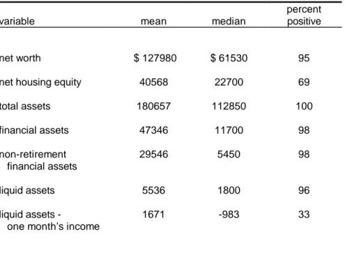
the variables come from cardholders’ monthly statements, credit bureau reports, or credit applications. To protect the identity of the accounts and the issuers, the data from different issuers were pooled together, with great care taken to define variables consistently across issuers. The results that are reported will focus on variables common to the issuers. Table 1 provides summary statistics for the main variables.
This data has a number of unique advantages compared to traditional household data sets like the SCF or the PSID. First, the large sample with little measurement error should provide much more power than usual to identify the effects of credit supply. Second, because each account is observed over many months, it is possible to study dynamics and control for fixed effects. This methodology will identify the idiosyncratic, within variation in a person’s debt associated with within variation in his credit line and interest rate. Third, unlike most studies, credit demand can be distinguished from credit supply. Not only do we separately observe credit limits, interest rates, and balances, we also know a great deal about the issuers’ underlying credit supply functions. This allows us to control for the endogeneity of the credit supply changes. The data contain essentially all the variables the issuers use to manage their accounts. Most notably we have access to each account’s credit scores, which are essentially the issuers’ own summary statistics for each account’s risk. With millions of accounts to manage, the issuers have largely automated their decision-making, relying very heavily on the scores in deciding credit policy for
each account (e.g., Moore, 1996).
Using account data does, however, entail a number of limitations. First, there is little information about some potentially important variables like household assets or employment status. However the issuers also lack access to this information, so its absence will not effect our approximately $500B of aggregate credit card debt evenly across the 3/4 of U.S. households with cards yields almost
identification strategy. Second, the main unit of analysis in the data is a credit card account, not an individual. We circumvent this limitation by using data from the credit bureaus, which cover all sources of credit used by the cardholder, in particular other credit card balances. (Gross and Souleles (1999) further describes the data.)
4. Econometric methodology
The results in this paper can be interpreted as an event study of how credit card debt responds to changes in credit supply, both in quantities and prices, over a period of about a year. However, since a given account can experience multiple changes over the year, especially multiple
interest rate changes, a distributed lag model is estimated. Let Di,t be the amount of debt held in
account i in month t, and let Li,t be the account’s credit limit (the line). The main specification
identifying the effect of changes in credit lines is equation (1):
∆Di,t = α'timet + βo∆Lit + β1∆Li,t-1 + β2∆Li,t-2 +… β12∆Li,t-12 + γ'Xit + εi,t, (1)
where ∆Di,t ≡Di,t - Di,t-1.The coefficient βo measures the contemporaneous increase in debt, per
dollar of line increase. This is the “impact effect” of liquidity. The marginal coefficients β1, β2, … ,
β12 measure the additional increases one month later, two months later, … , and twelve months
later, respectively. Consequently
∑
= ≡ k j j k b 0
β gives the cumulative increase in debt after k months,
k = 0-12. Twelve lags were sufficient for bkto converge. Attention will therefore focus on b12, the
total (long-run) effect on debt. b12 can be interpreted as the fraction of the line increase that is
$7000 of debt per household.
borrowed, or the long run “liquidity multiplier.” To identify the net aggregate effect of liquidity,
credit-bureau data on the balances held on other cards by account-holder i will also be used.
The dependent variable is the change in debt between months t-1 and t. Using differences
controls for individual effects in the level of debt. In the event study interpretation, i’s debt after
an increase in the credit line is being compared to his debt before the line increase. This identifies the within variation in a person’s debt due to within variation in his line. Furthermore, an explicit fixed effect will sometimes be added to equation (1), controlling for individual effects in the
growth in debt as well. This “second degree” fixed effect isolates an unusually powerful type of
variation. A complete set of month dummies, time, controls for all aggregate effects, including
seasonality and the business cycle, trends in debt over time, and aggregate interest rates.
About 4% of credit lines change in any given month. Unlike interest rates which both
increase and decrease, issuers are reluctant to decrease lines, so ∆L is non-negative. People who
do not receive a line increase in a given month remain in the sample that month with the
corresponding ∆L equal to zero. These people serve in a sense as a control group, in that the
estimated coefficients will pick up the effects of line changes relative to the debt of this group.
Sometimes additional control variables, X, will be added, usually with twelve lags corresponding
to the twelve lags for ∆L.
The specification for changes in interest rates r is analogous, except that only nine lags
were needed for convergence:
∆Di,t = α'timet + βo∆rit + β1∆ri,t-1 + β2∆ri,t-2 +… β12∆ri,t-9 + γ'Xit + εi,t . (2)
While the month dummies partial out aggregate interest rates, there remains substantial
their rates every few quarters. As a result about 20% of interest rates change in any given sample
month, both up and down. The coefficients βj identify the within variation in debt due to within
variation in interest rates. The cumulative coefficient b9 gives the total decrease in debt from a one
percentage point increase in the interest rate, i.e., the long-run semi-elasticity.
Equations (1) and (2) were estimated by OLS. The standard errors allow for heteroscedasticity across accounts as well as serial correlation within accounts. Various extensions will also be considered.
5. Results
This section first estimates the effects of credit line increases and then the effects of interest rate changes. In both cases the analysis begins with the main results for the credit card accounts in the sample. The analysis then turns to controlling for the endogeneity of the credit supply changes, explaining the heterogeneity in different people’s responses, and computing the total response in balances across all credit cards people hold, not only those in the sample.
a. Changes in credit limits
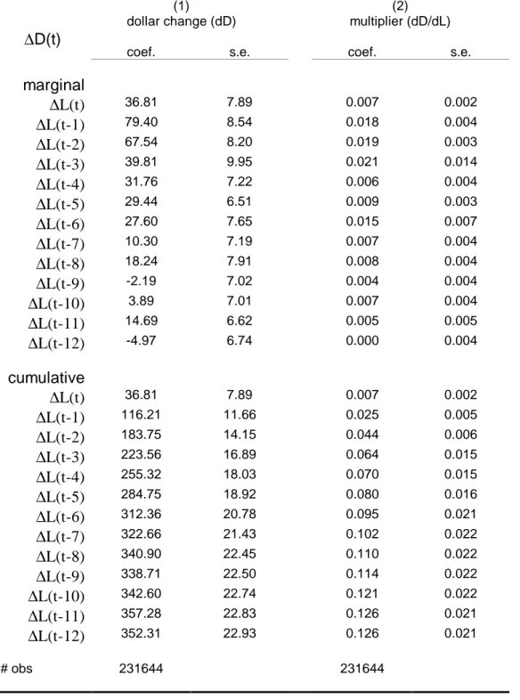
Table 2 records the main results for the line increase. As a starting point, in column (1) the
variables ∆Li,t-j in equation (1) have been replaced by dummy variables I(∆Li,t-j > 0), indicating
whether there was a line increase in the corresponding month. The estimated coefficients then
represent the dollar magnitudes of the resulting change in debt. The marginal coefficients βj in the
table are followed by the corresponding cumulative coefficients bk, which are also graphed in
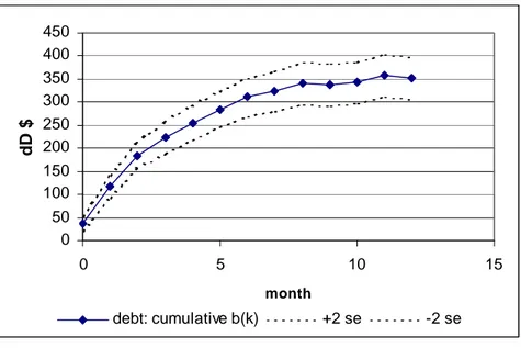
Figure 1. The impact effect βo is just under +40 and significant. On average debt rises by about
$80 and $70, and also significant. The corresponding cumulative coefficients b1 and b2 (graphed in
months 1 and 2 in the figure) show that debt rises sharply over the first two months after the line increase, to over $180. The marginal coefficients then begin to decay, becoming insignificant after
about 8 months; accordingly the cumulative coefficients begin to converge. The total effect b12 is
quite large and significant (with a t-ratio over 15): on average debt rises by over $350 in the year following a line increase. This is concrete evidence in favor of a consumer credit channel. Increases in liquidity generate immediate and large increases in spending and debt. The cumulative “impulse response” graphed in Figure 1 is remarkably smooth and easily significant. Such a result is rare in micro data. Presumably the difference is due to the large sample with little measurement error. The time dummies are also jointly significant. To save space they are not reported.
To gauge the magnitude of the liquidity multiplier, equation (1) is next estimated with the
original regressors ∆Li,t-j. The results appear in column (2) and are graphed in Figure 2. The
cumulative effect b12 converges to just under 0.13. Relative to the size of the line increase, on
average debt rises by almost 13%. In other words, each extra thousand dollars of liquidity generates a $130 increase in debt.
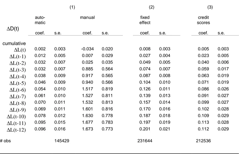
Table 3 shows the results of various extensions, beginning with an analysis of endogeneity.
(To save space, this and following tables will show only the cumulative coefficients bk.) For
instance, issuers may increase credit supply when they expect credit demand to be high. We employ a number of strategies to ensure that endogeneity is not driving the results. First, recall that the time dummies control for all aggregate effects. As a result, they control for the fact that issuers might offer additional credit before Christmas, for example, knowing that on average debt will subsequently rise. But the time dummies do not control for the analogous idiosyncratic situation in which, when people expect to make a big purchase in the near future, they call their
issuer and request a line increase. In this situation there would be reverse causality: the expected future purchases would be responsible for the line increase.
Fortunately, for a subset of our data we know whether the line increase was requested by the consumer or not. Such “manual” increases account for about 10% of the total number of line changes; the remaining 90% are automatically generated by a computer program. A dummy variable was created to identify which changes were manual, and this dummy and its twelve lags
were interacted with the line change ∆L and its lags in equation (1). Column (1) shows the
cumulative responses after both manual and automatic line changes. (The underlying dummy variables for manual changes, not shown, are jointly significant.) Not surprisingly debt rises much
more after a manual line increase. The total response b12 in that case is over 100% of the extra
line, though the standard errors are large because of the relatively small number of manual
changes. More interestingly the response of debt to automatic line changes is also significant. b12
remains large at about 0.10. Therefore, even though in the full sample we do not always know which line changes were automatic and which were manual, we do know that the small number of manual changes are not driving the results.
Second, issuers want to extend credit to people they think will borrow and pay interest but not default. They expend considerable resources to try to identify the characteristics of such people. Column (2) adds a fixed effect by account to equation (1), which controls for all
persistent characteristics of the account-holder. This is a fixed effect in the change in debt, which
should be a powerful control for endogeneity. Nonetheless the total multiplier b12 remains
significant and actually rises to 0.20.
Third, we control directly for the issuers’ credit supply policy, which to a first approximation is a function of the credit scores plus some exogenous timing rules described
below. As already noted, the credit scores are by far the most important variables determining credit policy for individual accounts. Many issuers use them essentially as summary statistics, so including them as independent variables goes a long way towards controlling for the endogeneity of the line changes. Since the distribution of scores is not uniform, they were first renormalized into deciles. This was done separately by issuer and then the deciles were interacted with dummy variables for the issuer, to allow each issuer to use their relative scores differently. These interacted variables were added to equation (1), along with twelve lags to control for the past line
changes.4 The results are in column (3). While the score variables are significant (not shown), they
do not materially change the main results. The total multiplier is over 0.11.
Fourth, credit issuers utilize some exogenous timing rules for changing the credit supply of different accounts. For example, some issuers will not consider (or are less likely to consider) an account for a line change if it has been less than six months or twelve months since the last line change. Thus, for a given account, the probability of a line change is much higher in certain months than in others. This suggests instrumenting for the line change with dummy variables for
the number of months since the last line change.5 These dummies and their lags were interacted
with issuer dummies, to allow each issuer to use different timing rules. The first-stage R2 is about
0.03, which is relatively large in the context of related micro studies. Again the main results, in column (4), do not change very much. The total multiplier rises slightly but remains about 0.13. Reassuringly, the pattern of coefficients remains smooth and the standard errors small. We
4
We also interacted these variables with time dummies, to allow each issuer to use the relative scores differently over time. Because of the large number of resulting regressors, we did this in smaller test samples. This time interaction had very little effect on the main results in the test samples.
5
Consider two people who are otherwise similar, but one had his last line increase 12 months ago, the other had it 11 months ago. The former is more likely to have his line go up this month. The IV estimates essentially compare his debt to the debt of the latter.
conclude that endogeneity is not driving the results. There appears to be a causal link from
liquidity to debt.6
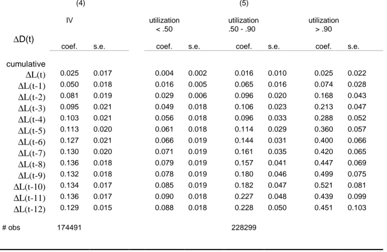
The results so far do not distinguish whether all people are responding equally to liquidity, or whether the response is limited to a few people. We now investigate the heterogeneity in different people’s responses. The goal is to identify why debt is responding to liquidity and what models of consumption and saving explain this response. To identify the role of liquidity constraints, we distinguish accounts according to their initial utilization rate, defined as balances
divided by the line. To avoid endogeneity, this rate is taken from month t-12, the beginning of the
distributed lag horizon in equation (1). The results appear in column (5) of Table 3. Indicator variables were created for accounts with initial utilization above 0.90 and for accounts between 0.50 and 0.90. The omitted category is initial utilization below 0.50. These indicators were
interacted with all lags of ∆L in equation (1). The two sets of interaction terms are each jointly
significant, so the response of debt varies with initial utilization rates. The people starting at over 90% utilization are potentially constrained, less than 10% of their credit line being free. Not surprisingly, they respond the most to additional liquidity: their debt rises by almost 50% of the
line increase (b12 > 0.45), significantly so. This sharp response suggests their liquidity constraints
are binding. More surprisingly, however, even the people starting at less than 50% utilization
respond significantly to additional liquidity. For them the total multiplier b12 is almost 0.09, and
quite significant. In dollar terms (estimated using the indicators I(∆Li,t-j > 0)), their debt rises by
about $200. This result seems inconsistent with a simple view of liquidity constraints. Consider
6
For comparison, recall that most previous studies have been unable to control much at all for the endogeneity of credit supply. Indeed, supply is usually not even separately observed from credit demand.
someone with a credit limit of $10,000 and a balance of $2500. Why should raising the limit to say $11,000 have any effect, given that the person was not constrained to begin with?
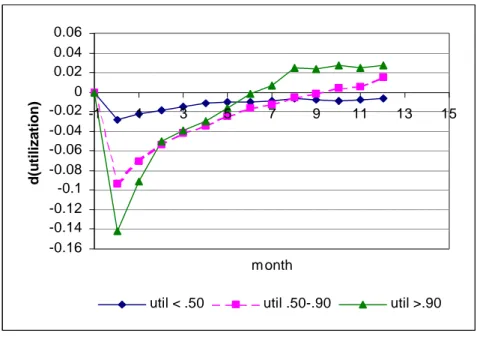
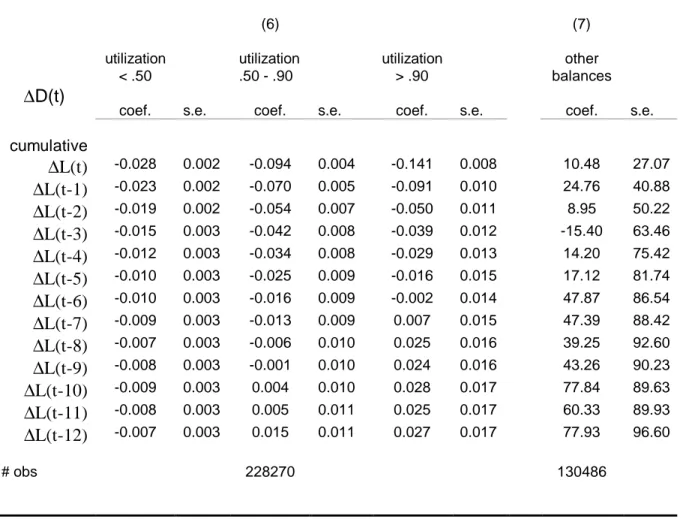
The results in column (6) suggest an answer. The dependent variable in equation (1) has
been changed to the utilization rate instead of debt (∆ utilizationi,t). The coefficients now give the
response of utilization after the line increase, separately by initial utilization as above. The cumulative effects are also graphed in Figure 3. In the month of the line increase (graphed in month 0), the utilization rates necessarily decline, because the line in the denominator of utilization has risen. The interesting issue is how quickly utilization recovers. Consider someone
who starts at 90% utilization. Since b0 is about -0.14, her utilization drops by 14 percentage
points, to 76%, in the month of the line change. But then the cumulative coefficients bk rise back
up towards zero. Within five months or so utilization is back near its original level, namely about 90% in this case. Interestingly, the same dynamics apply for the people who started with initially lower utilization. They too return back near their original utilization rates. These dynamics are consistent with people having “target” utilization rates.
While such targeting could be due to behavioral rules-of-thumb, it is also consistent with conventional precautionary motives, as in the models by Deaton (1991), Carroll (1992), and Ludvigson (1999). In these models agents worry not only about currently binding liquidity constraints, but also about constraints potentially binding in the future. In the language of Deaton, cash-on-hand should include the agent’s available line of credit. Such models generate an optimal level of cash-on-hand as a precautionary buffer stock against the possibility of future adverse shocks, and thereby they generate an optimal amount of credit to keep free. When the credit line rises, it is optimal to consume some of the extra liquidity, reserving only part of it for the buffer.
In particular it is possible for the optimal buffer of unused credit to be a constant fraction of the
line, which would generate a target utilization rate.7
However, conventional models will have more trouble explaining some other aspects of credit card use. Most saliently, why does such a large fraction of the population hold credit card debt, and why do so many of them simultaneously hold other assets yielding low returns? Table 4 describes the asset holdings of credit card borrowers, according to the 1995 SCF. Almost 60% of the SCF households that have credit cards (bank cards) report that they are borrowing on their cards. Of these households, 95% have positive net worth and so could in principle have paid off their expensive card debt by drawing down various assets. For instance, almost 70% have positive housing equity, and might be better off using lower cost home-equity debt. Over 90% have positive holdings of financial assets, even excluding illiquid, tax-favored retirement assets. Most puzzling of all, over 90% of people with credit card debt have some very liquid assets in checking and savings accounts. Granted, some transactions cannot easily be made using credit cards. (Though the ability to write checks against credit card accounts, or to take out cash advances, increases the scope of possible transactions.) Yet 1/3 of borrowers still have over one month’s worth of income in liquid assets, which is more than typically needed for cash transactions. These liquid assets could instead have been used to pay down their card debt. These results persist even for people with very substantial credit card debt. For over 10% of card-holding households, credit card debt amounts to more than one month’s income. Yet again about 1/3 of these high-debt households have over one month’s income in liquid assets.
7
This happens for instance in Ludvigson's model. It is homothetic in income because the credit constraint is scaled to income. However, this requires that lenders observe income at high frequency, and immediately decrease credit lines in response to decreases in income.
Such behavior is puzzling, and apparently inconsistent with no-arbitrage.8 Perhaps
behavioral models of mental accounts or self-control might help explain it. For example, some people might need to undertake costly actions to limit their “impulse” spending (or spending by their spouses). One example could be not fully paying off card balances, in order to reduce the
temptation of available credit.9 Alternatively, borrowers planning to file for bankruptcy have an
incentive to hold some assets, up to the amounts protected by the exemption rules. However such strategic bankruptcy planning should be undertaken only just before filing, to avoid paying unnecessary interest.
Finally, to determine the effect of line increases on the aggregate economy, it matters
whether net debt is increasing, or whether people are simply switching balances away from other
credit cards to the card in the sample with the new, larger credit line. Column (7) in Table 3
shows the results using other credit card balances as the dependent variable in equation (1). The
dummy variables I(∆Li,t-j > 0) are again used as regressors, so the coefficients show the
cumulative response of the other cards in dollars. Negative coefficients bk would represent an
offsetting decline in balances on other cards. The estimated coefficients are however insignificant and positive. Thus there is no offset from the other cards, so the previous results represent a net increase in debt, and hence have aggregate implications.
8
Insofar as people in the SCF underreport their credit card borrowing, these results will understate the magnitude of the credit card debt puzzle. We further explore these issues in a companion paper, Gross and Souleles (1999b).
9
More recently Laibson et. al. (1999) use hyperbolic discounting to explain simultaneously borrowing and saving for retirement (but cannot explain simultaneously borrowing and holding liquid, non-retirement assets). See also Laibson (1997) for a clever model of self-control in the presence of liquid and illiquid assets.
b. Changes in interest rates
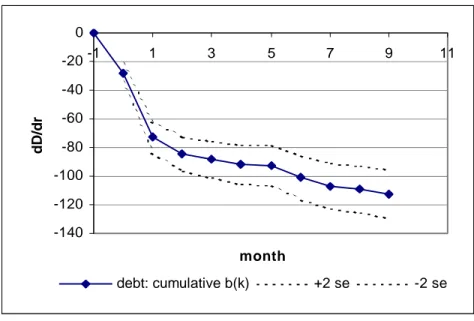
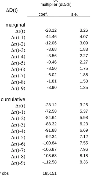
Table 5 records the main results for changes in interest rates, using equation (2), with the
cumulative coefficients graphed in Figure 4. The impact effect βo is almost -30 and the cumulative
effect after only one month b1 is -70. Thus debt responds immediately to interest rates: a one
percentage point increase in the interest rate leads on average to a $70 decline in debt after one
month. The total effect converges to around b9 = -112, a large and significant coefficient (with
t-ratio about 14). Thus higher interest rates do in fact lead to substantially less borrowing – people are sensitive to interest rates, the intertemporal elasticity of substitution is not zero. These numbers correspond to short-run and long-run elasticities of about -0.8 and -1.3, respectively. The cumulative "impulse response" in Figure 4 is again quite smooth and significant. These results are stronger and more robust than found in most other micro studies of interest-rate elasticities (both for consumers and for firms). We believe the difference is due to the large sample and reduced measurement error in our data, both in balances and in the interest rates, which are the account-specific marginal cost of funds.
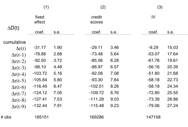
Table 6 displays various extensions, again beginning with endogeneity. In columns (1) and (2), including in equation (2) a fixed effect or the credit scores (with nine lags) does not substantially effect the results. As with credit limits, the issuers also use some arbitrary timing rules for changing interest rates. For instance, teaser rates usually expire after a fixed period like 6
months or 12 months, resulting in a large increase in rates at that time (e.g., from 5.9% to
15.9%). Rates on fixed rate cards can often only be changed once every couple quarters. Column (3) therefore instruments for the changes in rates with dummy variables for the number of months
smaller than before, at about -$80, but still significant. We conclude that endogeneity is not driving the result that debt is sensitive to the interest rate.
There are also large declines in interest rates in the data (e.g., from 15.9% to 5.9%), even though the sample consists of already open accounts. These declines are due to special promotional offers, which like introductory teasers usually end after fixed periods of time. Column (4) distinguishes the effects of large changes in interest rates from small changes, and of large increases from large decreases. Large increases are identified by indicator variables for the top 10% of the distribution of (non-zero) interest rate changes; large decreases by indicator variables for the bottom 10%. The baseline category is all other, smaller rate changes. Large decreases in rates have significantly stronger effects than other changes. Debt rises by over $120
per percentage point (b9 < -120), mostly in the first month. Large increases in rates are less
potent, but still depress debt more than small increases in rates; by about $70 compared to $45, respectively. These results suggest that large but temporary rate reductions can be effective in ratcheting up the amount of account debt. This can explain the widespread use of promotional
offers like teaser rates.10
The results also suggest the possibility that when rates change people are transferring balances between their card in the sample and their other cards. Column (5) uses other card
balances as the dependent variable in equation (2). Positive coefficients bk would represent
balance-shifting away from a card whose interest rate has increased. In fact the estimated total
effect b9 is almost +$40, and significant at the 6% level. Therefore there appears to be some
balance-shifting between cards. In other words people’s sensitivity to interest rates is large enough to overcome some switching costs. For each percentage point rise in the interest rate on
the card in the sample, while its balances decline by about $110, other card balances rise by about $40, for a net decline of $70 on average. Thus the balance-shifting is only partial; there is a net change in total borrowing. The net long-run elasticity is still large at about -0.85.
6. Conclusion
This paper has utilized a unique new data set of credit card accounts to analyze how people respond to changes in credit supply. We estimated the dynamic effects of changes in the credit limit and in interest rates, and considered the ability of different models of consumption and saving to rationalize these effects. The data set separately records credit limits and balances, allowing us to distinguish credit supply and demand, as well as account-specific interest rates. While measurement error might have thwarted previous studies of credit supply using traditional household data sets, it is not a problem here. As a result the “event studies” in this paper provide more powerful tests of the effects of credit supply than in most previous papers.
We find that increases in credit limits generate an immediate and significant rise in debt. This response is sharpest for people starting near their limit, providing evidence that liquidity constraints are binding. However, even people starting well below their limit significantly respond. We show this result is consistent with conventional models of precautionary savings. Nonetheless there are other results that conventional models cannot easily explain, such as the fact that many credit card borrowers simultaneously hold other low yielding assets. Unlike most other studies, we also find strong effects from changes in account-specific interest rates. Debt is particularly sensitive to large declines in interest rates, which can explain the widespread use of teaser rates. The long-run elasticity of debt to the interest rate is about -1.3. Less than half of this elasticity
10
represents balance-switching across cards, with most reflecting net changes in total borrowing. Overall, the results imply that the consumer plays a potentially important role in the transmission of monetary policy and other credit shocks.
We plan to extend this analysis in a number of ways. First, when issuers raise lines or lower interest rates, they are trading off larger interest payments with larger probabilities of default. In a companion paper, Gross and Souleles (1999), we estimated hazard models of default using the same data as in this paper. These two papers should be united to identify the profit-maximizing credit-supply function. Second, in terms of business cycle analysis, we have investigated only the second half of the consumer credit-supply channel, that is how people respond to changes in the supply of credit from lenders. Little is known about the first half of the channel, how credit card issuers and other consumer lenders change credit supply in response to monetary policy or other business cycle shocks.
Finally, more structural models of credit supply and demand can be constructed and calibrated. The results of this paper and the companion paper suggest a number of features that should be incorporated into such models. For instance, the unused line of credit serves as a precautionary buffer; consumers have the option to default but at the cost of restricting their future access to credit; the credit line and interest rate are endogenous functions of past borrowing behavior; there are wedges (possibly including those suggested by behavioral models) between the marginal costs of cash and credit making them imperfect substitutes in transactions.
7. References
Ausubel, L., 1991. “The Failure of Competition in the Credit Card Market,” American Economic
Review, v81, March, pp. 50-81.
Ausubel, L., 1999. “Adverse Selection in the Credit Card Market,” working paper, University of Maryland.
Bernanke, B., and Gertler, M., 1995. "Inside the Black Box: The Credit Channel of Monetary
Policy Transmission," Journal of Economic Perspectives, v9 #4, pp. 27-48.
Browning, M., and Lusardi, A., 1996. “Household Saving: Micro Theories and Micro Facts,”
Journal of Economic Literature, v34, December, pp. 1797-1855.
Chimerine, L., 1997. "Americans in Debt: The Reality," Mastercard International.
Calem, P., and Mester, L., 1995. “Consumer Behavior and the Stickiness of Credit Card Interest
Rates,” American Economic Review, v85 #5, pp. 1327-36.
Carroll, C., 1992. “The Buffer-Stock Theory of Saving: Some Macroeconomic Evidence,”
Brookings Papers on Economic Activity, v2, pp. 61-156.
Christiano, L., Eichenbaum, M., and Evans, C., 1996. "The Effects of Monetary Policy Shocks:
Evidence from the Flow of Funds," Review of Economics and Statistics, v78 #1, pp.
16-34.
Deaton, A., 1991. “Saving and Liquidity Constraints,” Econometrica, v59 #5, September, pp.
1221-48.
Federal Reserve Board, 1999. "G.19, Consumer Credit."
Gross, D., and Souleles, N., 1999. "An Empirical Analysis of Personal Bankruptcy and Delinquency," working paper, University of Chicago and University of Pennsylvania. Gross, D., and Souleles, N., 1999b. "How Do People Use Credit Cards?" working paper,
University of Chicago and University of Pennsylvania.
Gross, D., 1997. “The Investment and Financing Decisions of Liquidity Constrained Firms,” working paper, University of Chicago, June.
Hall, R., 1988. "Intertemporal Substitution in Consumption," Journal of Political Economy, 96,
pp. 339-57.
Jappelli, T., 1990. "Who Is Credit Constrained in the U.S. Economy?" Quarterly Journal of
Jappelli, T., Pischke, S., and Souleles, N., 1998. “Testing for Liquidity Constraints in Euler
Equations with Complementary Data Sources,” The Review of Economics and Statistics,
v80 #2, pp. 251-262.
Kashyap, A., and Stein, J., 1994. "Monetary Policy and Bank Lending," in Monetary Policy, ed.,
Mankiw, N., Chicago: University of Chicago Press.
Laibson, D, 1997. "Golden Eggs and Hyperbolic Discounting." Quarterly Journal of Economics,
May, v112 #2, pp. 443-477.
Laibson, D., Repetto, A., and Tobacman, J., 1999. “A Debt Puzzle," working paper, Harvard University.
Ludvigson, S., 1998. “The Channel of Monetary Transmission to Demand: Evidence from the
Market for Automobile Credit,” Journal of Money, Credit, and Banking, August, pp.
365-383.
Ludvigson, S., 1999. “Consumption and Credit: A Model of Time-Varying Liquidity
Constraints,” The Review of Economics and Statistics, August, pp. 434-447.
Moore, M., 1996. “Credit Scoring’s Uses Expand as It Gains Acceptance,” The American
Banker, June 4, p. 4A.
Mishkin, F., 1995. "Symposium on the Monetary Transmission Mechanism," Journal of
Economics Perspectives, v9 #4, pp. 3-10.
Yoo, P., 1998. “Still Charging: The Growth of Credit Card Debt between 1992 and 1995."
Federal Reserve Bank of St. LouisReview, January/February, pp. 19-27.
Zeldes, S., 1989. "Consumption and Liquidity Constraints: An Empirical Investigation." Journal
Figure 1. The cumulative response of debt to increases in the credit limit, in dollars.
Figure 2. The cumulative response of debt to increases in the credit limit, per dollar of extra line.
0 0.02 0.04 0.06 0.08 0.1 0.12 0.14 0.16 0.18 0.2 0 5 10 15 month dD/dL debt: cumulative b(k) +2 se -2 se 0 50 100 150 200 250 300 350 400 450 0 5 10 15 month dD $ debt: cumulative b(k) +2 se -2 se
Figure 3. The cumulative response of utilization to increases in the credit limit, by initial utilization rate. -0.16 -0.14 -0.12 -0.1 -0.08 -0.06 -0.04 -0.02 0 0.02 0.04 0.06 -1 1 3 5 7 9 11 13 15 m onth d(utilization)
Figure 4. The cumulative response of debt to changes in the interest rate, per percentage point. -140 -120 -100 -80 -60 -40 -20 0 -1 1 3 5 7 9 11 month dD/dr debt: cumulative b(k) +2 se -2 se
Table 2. The Response of Debt to Increases in the Credit Limit (1) dollar change (dD) (2) multiplier (dD/dL) ∆D(t)
coef. s.e. coef. s.e.
marginal ∆L(t) 36.81 7.89 0.007 0.002 ∆L(t-1) 79.40 8.54 0.018 0.004 ∆L(t-2) 67.54 8.20 0.019 0.003 ∆L(t-3) 39.81 9.95 0.021 0.014 ∆L(t-4) 31.76 7.22 0.006 0.004 ∆L(t-5) 29.44 6.51 0.009 0.003 ∆L(t-6) 27.60 7.65 0.015 0.007 ∆L(t-7) 10.30 7.19 0.007 0.004 ∆L(t-8) 18.24 7.91 0.008 0.004 ∆L(t-9) -2.19 7.02 0.004 0.004 ∆L(t-10) 3.89 7.01 0.007 0.004 ∆L(t-11) 14.69 6.62 0.005 0.005 ∆L(t-12) -4.97 6.74 0.000 0.004 cumulative ∆L(t) 36.81 7.89 0.007 0.002 ∆L(t-1) 116.21 11.66 0.025 0.005 ∆L(t-2) 183.75 14.15 0.044 0.006 ∆L(t-3) 223.56 16.89 0.064 0.015 ∆L(t-4) 255.32 18.03 0.070 0.015 ∆L(t-5) 284.75 18.92 0.080 0.016 ∆L(t-6) 312.36 20.78 0.095 0.021 ∆L(t-7) 322.66 21.43 0.102 0.022 ∆L(t-8) 340.90 22.45 0.110 0.022 ∆L(t-9) 338.71 22.50 0.114 0.022 ∆L(t-10) 342.60 22.74 0.121 0.022 ∆L(t-11) 357.28 22.83 0.126 0.021 ∆L(t-12) 352.31 22.93 0.126 0.021 # obs 231644 231644 Notes:
• In column (1), the regressors are the indicators I(∆L>0).
• Month dummies not shown. Standard errors allow for heteroscedasticity across accounts as well as serial correlation within accounts.
Table 3. Extensions for the Credit Limit (1) (2) (3) auto-matic manual fixed effect credit scores ∆D(t)
coef. s.e. coef. s.e. coef. s.e. coef. s.e.
cumulative ∆L(t) 0.002 0.003 -0.034 0.020 0.008 0.003 0.005 0.003 ∆L(t-1) 0.012 0.005 0.007 0.029 0.027 0.004 0.023 0.005 ∆L(t-2) 0.032 0.007 0.025 0.035 0.049 0.005 0.040 0.006 ∆L(t-3) 0.032 0.007 0.885 0.564 0.074 0.007 0.059 0.017 ∆L(t-4) 0.038 0.009 0.917 0.565 0.087 0.008 0.063 0.019 ∆L(t-5) 0.046 0.009 0.940 0.566 0.104 0.010 0.071 0.019 ∆L(t-6) 0.054 0.010 1.517 0.819 0.126 0.011 0.086 0.026 ∆L(t-7) 0.061 0.010 1.527 0.811 0.139 0.013 0.091 0.027 ∆L(t-8) 0.070 0.011 1.532 0.813 0.157 0.014 0.099 0.027 ∆L(t-9) 0.069 0.011 1.601 0.816 0.170 0.016 0.102 0.028 ∆L(t-10) 0.078 0.012 1.630 0.778 0.187 0.018 0.109 0.029 ∆L(t-11) 0.095 0.015 1.677 0.783 0.197 0.019 0.113 0.028 ∆L(t-12) 0.096 0.016 1.673 0.773 0.201 0.021 0.112 0.029 # obs 145429 231644 212536
Table 3. Extensions for the Credit Limit (ctd.) (4) (5) IV utilization < .50 utilization .50 - .90 utilization > .90 ∆D(t)
coef. s.e. coef. s.e. coef. s.e. coef. s.e.
cumulative ∆L(t) 0.025 0.017 0.004 0.002 0.016 0.010 0.025 0.022 ∆L(t-1) 0.050 0.018 0.016 0.005 0.065 0.016 0.074 0.028 ∆L(t-2) 0.081 0.019 0.029 0.006 0.096 0.020 0.168 0.043 ∆L(t-3) 0.095 0.021 0.049 0.018 0.106 0.023 0.213 0.047 ∆L(t-4) 0.103 0.021 0.056 0.018 0.096 0.033 0.288 0.052 ∆L(t-5) 0.113 0.020 0.061 0.018 0.114 0.029 0.360 0.057 ∆L(t-6) 0.127 0.021 0.066 0.019 0.144 0.031 0.400 0.066 ∆L(t-7) 0.130 0.020 0.071 0.019 0.161 0.035 0.420 0.065 ∆L(t-8) 0.136 0.018 0.079 0.019 0.157 0.041 0.447 0.069 ∆L(t-9) 0.132 0.018 0.078 0.019 0.180 0.046 0.499 0.075 ∆L(t-10) 0.134 0.017 0.085 0.019 0.182 0.047 0.521 0.081 ∆L(t-11) 0.136 0.017 0.090 0.018 0.227 0.048 0.439 0.099 ∆L(t-12) 0.129 0.015 0.088 0.018 0.228 0.050 0.451 0.103 # obs 174491 228299
Table 3. Extensions for the Credit Limit (ctd.) (6) (7) utilization < .50 utilization .50 - .90 utilization > .90 other balances ∆D(t)
coef. s.e. coef. s.e. coef. s.e. coef. s.e.
cumulative ∆L(t) -0.028 0.002 -0.094 0.004 -0.141 0.008 10.48 27.07 ∆L(t-1) -0.023 0.002 -0.070 0.005 -0.091 0.010 24.76 40.88 ∆L(t-2) -0.019 0.002 -0.054 0.007 -0.050 0.011 8.95 50.22 ∆L(t-3) -0.015 0.003 -0.042 0.008 -0.039 0.012 -15.40 63.46 ∆L(t-4) -0.012 0.003 -0.034 0.008 -0.029 0.013 14.20 75.42 ∆L(t-5) -0.010 0.003 -0.025 0.009 -0.016 0.015 17.12 81.74 ∆L(t-6) -0.010 0.003 -0.016 0.009 -0.002 0.014 47.87 86.54 ∆L(t-7) -0.009 0.003 -0.013 0.009 0.007 0.015 47.39 88.42 ∆L(t-8) -0.007 0.003 -0.006 0.010 0.025 0.016 39.25 92.60 ∆L(t-9) -0.008 0.003 -0.001 0.010 0.024 0.016 43.26 90.23 ∆L(t-10) -0.009 0.003 0.004 0.010 0.028 0.017 77.84 89.63 ∆L(t-11) -0.008 0.003 0.005 0.011 0.025 0.017 60.33 89.93 ∆L(t-12) -0.007 0.003 0.015 0.011 0.027 0.017 77.93 96.60 # obs 228270 130486 Notes:
• Month dummies and marginal coefficients not shown. Sample size can vary with missing variables and different samples. Standard errors allow for heteroscedasticity across accounts as well as serial correlation within accounts.
• In column (3), the credit scores are not shown.
• In columns (5) and (6), separate intercepts for each utilization group are not shown. In column (6), the dependent variable is the utilization rate.
• In column (7), the dependent variable is balances on other credit cards, and the independent variables are the indicators I(∆L >0).
Table 4: Asset Holdings of Credit Card Borrowers
variable mean median
percent positive
net worth $ 127980 $ 61530 95 net housing equity 40568 22700 69 total assets 180657 112850 100 financial assets 47346 11700 98 non-retirement financial assets 29546 5450 98 liquid assets 5536 1800 96 liquid assets
one month’s income
1671 -983 33
Notes:
• Source: 1995 SCF.
• Results are weighted to be representative, and for comparison include only bank-card debt (e.g., Visa and Mastercard), not retail and travel/entertainment cards (e.g., American Express). All results are conditional on having and borrowing on at least one bank card.
• Asset definitions generally follow standard SCF codebook suggestions, with the exception that net worth does not include credit card debt. Non-retirement financial assets exclude IRA’s and defined-contribution pensions. Liquid assets include amounts in checking, saving, money-market, and brokerage call accounts. Income is gross total household income.
Table 5. The Response of Debt to Changes in Interest Rates (1) multiplier (dD/dr) ∆D(t) coef. s.e. marginal ∆r(t) -28.12 3.26 ∆r(t-1) -44.46 4.07 ∆r(t-2) -12.06 3.09 ∆r(t-3) -3.68 1.83 ∆r(t-4) -3.56 2.27 ∆r(t-5) -0.46 2.27 ∆r(t-6) -8.50 1.75 ∆r(t-7) -6.02 1.88 ∆r(t-8) -1.81 1.53 ∆r(t-9) -3.90 1.35 cumulative ∆r(t) -28.12 3.26 ∆r(t-1) -72.58 5.37 ∆r(t-2) -84.64 5.98 ∆r(t-3) -88.32 6.23 ∆r(t-4) -91.88 6.69 ∆r(t-5) -92.34 7.12 ∆r(t-6) -100.84 7.55 ∆r(t-7) -106.87 7.96 ∆r(t-8) -108.68 8.18 ∆r(t-9) -112.58 8.36 # obs 185151 Notes:
• Month dummies not shown. Standard errors allow for heteroscedasticity across accounts as well as serial correlation within accounts.
Table 6. Extensions for Interest Rates (1) (2) (3) fixed effect credit scores IV ∆D(t)
coef. s.e. coef. s.e. coef. s.e.
cumulative ∆r(t) -31.17 1.90 -29.11 3.46 -9.29 15.03 ∆r(t-1) -78.88 2.88 -73.48 5.64 -53.07 17.64 ∆r(t-2) -92.50 3.72 -85.06 6.28 -61.76 19.61 ∆r(t-3) -98.10 4.48 -88.97 6.57 -56.16 20.39 ∆r(t-4) -103.72 5.16 -92.08 7.08 -51.80 21.68 ∆r(t-5) -105.84 5.80 -93.30 7.64 -58.18 22.73 ∆r(t-6) -116.49 6.47 -102.51 8.26 -58.18 24.34 ∆r(t-7) -124.12 7.05 -109.72 8.76 -72.80 25.55 ∆r(t-8) -127.41 7.53 -111.28 9.03 -73.39 26.86 ∆r(t-9) -132.44 7.91 -115.48 9.23 -79.06 27.24 # obs 185151 169286 147158
Table 6. Extensions for Interest Rates (ctd.) (4) (5) small changes large increases large decreases other balances ∆D(t)
coef. s.e. coef. s.e. coef. s.e. coef. s.e.
cumulative ∆r(t) -25.67 8.74 -14.43 4.71 -41.29 5.12 1.90 6.46 ∆r(t-1) -39.40 12.09 -28.18 6.30 -118.53 8.50 -14.12 11.20 ∆r(t-2) -45.91 14.33 -39.53 7.05 -128.86 9.23 -5.63 13.37 ∆r(t-3) -45.27 15.83 -42.72 7.99 -130.18 9.37 8.45 15.04 ∆r(t-4) -55.53 17.49 -49.70 8.81 -127.26 9.72 19.98 16.21 ∆r(t-5) -54.94 18.64 -52.81 9.17 -122.32 10.33 27.94 17.05 ∆r(t-6) -55.24 19.23 -57.82 9.40 -131.88 10.83 34.02 17.89 ∆r(t-7) -51.74 20.23 -62.30 9.54 -132.73 11.69 31.22 18.64 ∆r(t-8) -50.50 22.69 -65.19 9.64 -128.68 12.23 36.44 19.70 ∆r(t-9) -44.75 22.85 -71.11 9.71 -126.36 12.78 37.83 20.17 # obs 185151 142334 Notes:
• Month dummies and marginal coefficients not shown. Sample size can vary with missing variables and different samples. Standard errors allow for heteroscedasticity across accounts as well as serial correlation within accounts. • In column (2), the credit scores are not shown.
• In column (4), separate intercepts for the different magnitudes of rate changes are not shown. • In column (5), the dependent variable is balances on other credit cards.
