Clemson University
TigerPrints
All Dissertations
Dissertations
12-2015
Objective Bayesian analysis on the quantile
regression
Shiyi Tu
Clemson University, [email protected]
Follow this and additional works at:
https://tigerprints.clemson.edu/all_dissertations
Part of the
Statistics and Probability Commons
This Dissertation is brought to you for free and open access by the Dissertations at TigerPrints. It has been accepted for inclusion in All Dissertations by an authorized administrator of TigerPrints. For more information, please [email protected].
Recommended Citation
Tu, Shiyi, "Objective Bayesian analysis on the quantile regression" (2015).All Dissertations. 1544.
OBJECTIVE BAYESIAN ANALYSIS ON THE QUANTILE REGRESSION
A Dissertation Presented to the Graduate School of
Clemson University
In Partial Fulfillment
of the Requirements for the Degree Doctor of Philosophy Mathematical Sciences by Shiyi Tu December 2015 Accepted by:
Dr. Xiaoqian Sun, Committee Chair Dr. Derek Brown
Dr. Colin Gallagher Dr. Yingbo Li
Abstract
The dissertation consists of two distinct but related research projects. First of all, we study the Bayesian analysis on the two-piece location-scale models, which contain several well-known sub-distributions, such as the asymmetric Laplace distribution, the-skew normal distribution, and the skewed Student-tdistribution. The use of two-piece location-scale models is an attractive method to model non-symmetric data. From a practical point of view, a prior with some objective information may be more reasonable due to the lack of prior information in many applied situations. It has been shown that several common used objective priors, such as the Jeffreys prior, result in improper posterior distributions for the case of two-piece location-scale models. This motivates us to consider alternative priors. Specifically, we develop reference priors with partial information which lead to proper posterior distributions. Based on those priors, we extend our prior to a general class of priors. A sufficient and necessary condition is provided to ensure the propriety of the posterior
distribution under such general priors. Our results show that the proposed Bayesian approach
outperforms the frequentist method in terms of mean squared error. It is noteworthy that the proposed Bayesian method can be applied to the quantile regression due to the close relationship between the asymmetric Laplace distribution and the quantile regression.
The second project deals with the Bayesian variable selection for the maximum entropy quantile regression. Quantile regression has gained increasing popularity in many areas as it provides richer information than the regular mean regression, and variable selection plays an important role in quantile regression model building process, as it can improve the prediction accuracy by choosing an appropriate subset of regression predictors. Most existing methods in quantile regression consider quantile at some fixed value. However, if our purpose is, among all the fitted quantile regression models, to identify which one fits the data best, then the traditional quantile regression may not be appropriate. Therefore, we consider the quantile as an unknown parameter and estimate it
jointly with other regression coefficients. In particular, we consider the maximum entropy quantile regression whose error distribution is obtained by maximizing Shannon’s entropy measure subject to two moment constraints. We apply the Bayesian adaptive Lasso to the model and put a flat prior on the quantile parameter due to the lack of information on it. Our proposed method not only addresses the problem about which quantile would be the most probable one among all the candidates, but also reflects the inner relationship of the data through the estimated quantile. We develop an efficient Gibbs sampler algorithm and show that the results of our proposed method are better than the ones under the Bayesian Lasso and Bayesian adaptive Lasso with fixed quantile values through both simulation studies and real data analysis.
Dedication
This dissertation is dedicated to my parents, Liping Peng and Jiangang Tu, who love me, believe in me, inspire me and have supported me every step of the way.
Acknowledgments
First and foremost, I would like to show my deepest gratitude to my advisor, Dr. Xiaoqian Sun, a respectable, responsible and resourceful scholar, who has provided me with valuable guidance on my graduate studies and research projects. I could not have completed my work without his inspiration and support.
I would specially like to thank Dr. Derek Brown, Dr. Colin Gallagher and Dr. Yingbo Li for their advice, support and serving on my advisory committee. They provided many valuable suggestions in my proposal defense for me to complete this work. In addition, I would thank to Dr. Cox and Kris for their help during my stay at the Department of Mathematical Sciences, Clemson University.
I have recently submitted one dissertation-derived paper for peek review. In addition, one dissertation-derived paper has been accepted for publication byComputational Statistics and Data Analysis. I am very grateful to the editor, the associate editor, and the anonymous referees of this journal for their constructive suggestions that led to the improvements of this paper.
I would also like to thank Dewei Wang and his wife Chendi Jiang, Dongmei Wang, Min Wang, Qi Zheng, and Haiming Zhou for continuously offering me help since I came to U.S.A. Especially, I am thankful to Xiaohua Bai, Yan Liu, Yanbo Xia, Honghai Xu, Shuhan Xu, Yibo Xu and his wife Xun Dong, Jing Zhao and his wife Jinghua Zhao for their support and encouragement. Last but not least, I would like to thank my parents, my wife Jingshu for their love, under-standing, support and assistance through my study.
Table of Contents
Title Page . . . i
Abstract . . . ii
Dedication . . . iv
Acknowledgments . . . v
List of Tables . . . vii
List of Figures . . . viii
1 Introduction . . . 1
2 Bayesian Analysis of Two-piece Location-scale Models under Reference Priors with Partial Information . . . 4
2.1 Introduction . . . 4
2.2 Two-piece location-scale models and reparametrization . . . 6
2.3 Reference priors with partial information . . . 8
2.4 Simulation study and real data analysis . . . 21
2.5 Concluding remarks . . . 25
2.6 Proofs . . . 26
3 Variable Selection in Quantile Regression . . . 29
3.1 Quantile regression . . . 29
3.2 Frequentist variable selection in the quantile regression . . . 31
3.3 Bayesian variable selection in the quantile regression . . . 38
3.4 Discussion . . . 57
4 Variable Selection in Bayesian Maximum Entropy Quantile Regression . . . 59
4.1 Introduction . . . 59
4.2 Maximum entropy quantile regression . . . 62
4.3 Bayesian adaptive Lasso on the maximum entropy quantile regression . . . 64
4.4 Simulation study . . . 69
4.5 Real data analysis . . . 74
4.6 Concluding Remarks . . . 81
5 Future Work . . . 83
5.1 Bayesian binary quantile regression . . . 83
5.2 Bayesian logistic quantile regression . . . 85
List of Tables
2.1 Scenarios of the RPPI in two-piece location-scale models. . . 10 2.2 MSEs of each parameter whenn= 100. . . 22
2.3 Bayesian estimates and MLEs with corresponding standard deviations (sd) in
paren-thesis when sample size is 100. . . 22 2.4 Acceptance rates for the Metropolis step when n=100. . . 24 2.5 Frequentist converge probability of 95% CI. . . 25
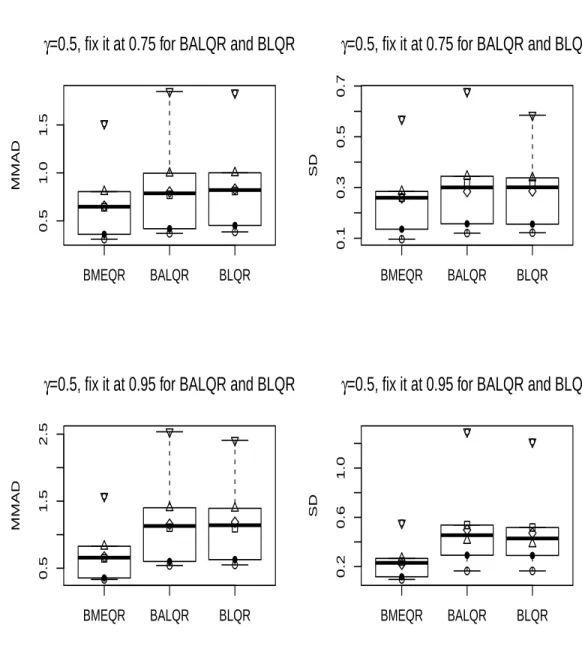
4.1 The parameter estimates for the simulated data with normally distributed errors and
the corresponding standard deviations in the parenthesis. The true value ofγis 0.95, whereas we set it to be 0.5 for BALQR and BLQR. . . 73
List of Figures
2.1 Examples of the ALD . . . 14
2.2 The marginal priors forγ . . . 15
2.3 Boxplots summarizing the Bayesian estimates and MLE ofµ, and the corresponding standard deviations whenγ= 0.2 and sample size is 100. . . 23
2.4 Boxplots summarizing the Bayesian estimates and MLE ofσ, and the corresponding standard deviations whenγ= 0.2 and sample size is 100. . . 23
2.5 Boxplots summarizing the Bayesian estimates and MLE ofγ, and the corresponding standard deviations of them whenγ= 0.2 and sample size is 100. . . 24
2.6 Fitted curves and data histogram: Bayesian predictive density curve (Bayesian), and MLEs based curve (MLE). . . 25
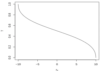
4.1 Graph ofγ(r2) whenr1= 10. . . 64
4.2 Boxplots summarizing the MMADs and the corresponding standard deviations under the three methods for the six error distributions in Simulation 1 whenγis 0.5. Over-laid are AL (), normal distribution (◦), normal mixture (4), Laplace (♦), Laplace mixture (∇), andt distribution (•). . . 71
4.3 Boxplots summarizing the MMADs and the corresponding standard deviations under the three methods for the six error distributions in Simulation 3 when γ is 0.95. Overlaid are AL (), normal distribution (◦), normal mixture (4), Laplace (♦), Laplace mixture (∇), andt distribution (•). . . 72
4.4 Posterior distributions of (β1, β2, β3, β4) overplotted with the histogram of simulated values in BMEQR. . . 74
4.5 Posterior distributions of (β5, β6, β7, β8) overplotted with the histogram of simulated values in BMEQR. . . 75
4.6 Boxplots summarizing simulated γ and the corresponding standard deviation for BMEQR using the six error distributions in Simulation 1. Overlaid are AL (), normal distribution (◦), normal mixture (4), Laplace (♦), Laplace mixture (∇), and tdistribution (•). . . 76
4.7 Boxplots summarizing simulated γ and the corresponding standard deviation for BMEQR using the six error distributions in Simulation 2. Overlaid are AL (), normal distribution (◦), normal mixture (4), Laplace (♦), Laplace mixture (∇), and tdistribution (•). . . 77
4.8 Boxplots summarizing simulatedγand corresponding standard deviation for BMEQR using the six error distributions in Simulation 3. Overlaid are the AL (), normal distribution (◦), normal mixture (4), Laplace (♦), Laplace mixture (∇), and t dis-tribution (•). . . 78
4.9 Boxplots summarizing the MSE of the three methods whenγ= 0.1. . . 79
4.10 Boxplots summarizing the MSE of the three methods whenγ= 0.3. . . 80
4.11 Boxplots summarizing the MSE of the three methods whenγ= 0.5. . . 80
Chapter 1
Introduction
The dissertation consists of two distinct but related research projects. The first project deals with the problems of point estimation and frequentist coverage probability for the parameters in the two-piece location-scale models. The second project discusses the variable selection for the maximum entropy quantile regression through Bayesian adaptive Lasso.
In Chapter 2, we consider the Bayesian approach to the point estimation for the parame-ters in the two-piece location-scale models. Numerous researchers have discussed those models by adopting subjective priors for the parameters. However, from a practical point of view, a prior with some objective information may be more reasonable due to the lack of prior information in many situations. The most common used objective prior is the Jeffreys prior. Recently, [47] derived the Jeffreys and independence Jeffreys priors for the two-piece location-scale models. Unfortunately, it has been shown that these Jeffreys priors result in improper posterior distributions for some sub-models, such as the inverse scale factors model. It is well known that the Bayesian inference on an improper posterior distribution is invalid. Therefore, the Jeffrey priors can not be used for the two-piece location-scale models. Another common used objective prior is the reference priors, which are very difficult to calculate for the two-piece location-scale models. As an alternative way, we consider using reference priors with partial information, which share the same idea as the reference priors, and are easier to derive. We derive several references priors with partial information for the two-piece location-scale models, and discuss the propriety of the posterior distributions for one special case of the models, the asymmetric Laplace distribution (ALD). We have also proposed similar results for the other two sub-models, the inverse scale factors model, and the -skew model. A sufficient and
necessary condition has been established to ensure the propriety of the posterior distribution under a general class of priors for the ALD. The results of the Bayesian approach are compared with the maximum likelihood estimators.
The close relationship between the ALD and the quantile regression is studied by [61]. Consider the linear model y=Xβ+, the γth quantile regression is defined as any solutionβ(γ)
that minimizing P
iργ(yi−xiβ), where ργ(·) is the check function. If we consider the ALD as the error distribution for the above linear model, then the maximum likelihood estimators (MLE)
of regression coefficients β is the solution to the above minimization problem. Thus we can use
Bayesian approach to estimateβand the method we discuss in Chapter 2 can be naturally extended
to the quantile regression.
When the model contains many predictors, variable selection plays an important role in the model building process to obtain a better interpretation and to improve the precision of model fit. In Chapter 3, we review several variable selection methods in the quantile regression, ranging from the frequentist approaches to the Bayesian procedures. All of those methods estimate the regression coefficients at some fixed quantile value. However, if our purpose is, among all the quantile regression models, to identify which one fits the data best, then the traditional quantile regression may not be appropriate. For example, given a range of quantile, (0.1,0.2,· · · ,0.9), we could fit 9 different regression models according to each quantile value, we are interested in which one is the most probable one to exact the most information from the data. That is, which model could reflect the inner relationship of the data and which quantile would be the most likely one. In such cases, those questions can be easily answered if we consider the quantile as an unknown parameter and estimate it from the data. Therefore, in order to extract important information from the data itself, we consider the quantile as an unknown parameter and estimate it jointly with other regression coefficients. The detail algorithm is discussed in Chapter 4.
In Chapter 4, we consider the Bayesian approach to the problem of variable selection on the maximum entropy quantile regression. Although the error distribution of the quantile regression is usually unknown, it is restricted to be 0 at a specified quantile level. We consider a special error distribution by maximizing Shannon’s entropy measure subject to two moment constraints, and refer the resulting model to the maximum entropy quantile regression. The Bayesian adaptive Lasso has been employed to the variable selection on the maximum entropy quantile regression. We consider the quantile as an unknown parameter and put a uniform prior on it. Our proposed method not
only addresses the problem about which quantile would be the most probable one among all the candidates, but also reflects the inner relationship of the data through the estimated quantile. The results presented here are compared with the ones through Bayesian Lasso and Bayesian adaptive Lasso with fixed quantile value.
Some future work are discussed in Chapter 5. We consider extending the method in Chap-ter 4 to other types of quantile regression, such as the binary quantile regression, and the logistic quantile regression.
Chapter 2
Bayesian Analysis of Two-piece
Location-scale Models under
Reference Priors with Partial
Information
2.1
Introduction
The use of skewed distributions is an attractive option for modeling data when symmetry is not appropriate; see, for example, [6], [49], [26], among others. As an illustration, it is widely known that the asymmetric Laplace distribution (ALD), a special case of this family, has received much attention in a wide range of disciplines, such as economics ([65]), engineering ([32]), financial analysis ([33]), medical study ([42]), and microbiology ([46]). In recent years, numerous techniques have been developed to derive new skewed distributions, mainly based on a modification of various symmetric distributions, such as adding a scale parameter to the symmetric density ([18]), multiplying the original density by a cumulative density function of a symmetric random variable ([40]).
Due to their simplicity and fitting real data quite well in practice, the two-piece location-scale models have been paid considerable attention in the literature. Besides the ALD, other two of
their special sub-models, the inverse scale factors model and the-skew model, have been discussed extensively by [18] and then by [39]. In the absence of prior knowledge, an objective prior such as the Jeffreys prior is often preferred to conduct Bayesian inference. Recently, [47] derived the Jeffreys and independence Jeffreys priors for several families of the skewed distributions. Unfortunately, it has been shown that these Jeffreys priors result in improper posterior distributions for some sub-models, such as the inverse scale factors model. Of particular note is that from [47], several discussants advocated the use of reference priors proposed by [10], which are very difficult to calculate for the two-piece location-scale models. However, reference priors with partial information (for short, RPPI) firstly proposed by [52] share the same idea as reference priors, and are easier to derive. Therefore, we are interested in deriving RPPI to see if they result in proper posterior distributions.
The use of RPPI is also quite attractive in applied situations because we usually have some partial prior information for several parameters. Thus, we just need to find a conditional prior for the remaining unknown parameters based on available information. For instance, [11] showed that for the range parameter in the spatial model, the frequentist coverage probability of the credible intervals based on the RPPI is better than the one in terms of the Jeffreys prior. [19] illustrated that for elapsed times in continuous-time Markov chains, the frequentist coverage of the credible intervals of the parameters based on the RPPI are better than the ones from other priors. [14] discussed Bayesian inference for the high energy physics problems by applying the RPPI for both single-count and multiple-count models and obtained a nice frequentist coverage probability. In this chapter, we derive RPPI for the two-piece location-scale models and show that some of them lead to proper posterior distributions. In particular, a sufficient and necessary condition for the propriety of the posterior distribution is provided under a general class of priors.
The reminder of this chapter is organized as follows. In Section 2.2, we describe the two-piece location-scale models and present several skewed distributions from different reparametrizations. In Section 2.3, we derive several RPPI for these distributions and study the propriety of the posterior distributions for the ALD in detail. In Section 2.4, the performance of our approach is illustrated through extensive simulation studies and one real data application. Finally, some concluding remarks are provided in Section 2.5, with proofs given in Section 2.6.
2.2
Two-piece location-scale models and reparametrization
The framework of the two-piece location-scale models was established by [47]. For com-pleteness, we firstly overview such models as follows. Letf(y|µ, σ) be a symmetric and absolutely continuous density with support onR, location parameterµ∈R, and scale parameterσ∈R+. The
probability density function (pdf) of these models has the form:
h(y|µ, σ1, σ2, ) = 2 σ1 f(y|µ, σ1)I(−∞,µ)(y) + 2(1−) σ2 f(y|µ, σ2)I[µ,∞)(y),
where σ1 ∈ R+ and σ2 ∈ R+ are two separate scale parameters, and 0 < < 1. Note that the
densityh(·) is the finite mixtures of the densities obtained by truncating the location-scale densities f(y|µ, σ1) andf(y|µ, σ2) at the intervals (−∞, µ] and [µ,∞), respectively. Therefore, the density
h(·) may not be continuous aty=µ. In order to ensure the continuity of the density, we setto be σ1/(σ1+σ2). Consequently, the above density can be rewritten as
g(y|µ, σ1, σ2) = 2 σ1+σ2 f(y|µ, σ1)I(−∞,µ)(y) +f(y|µ, σ2)I[µ,∞)(y) . (2.1) Note that Z µ −∞ g(y|µ, σ1, σ2)dy= σ1 σ1+σ2 ,
which indicatesg(·) is skewed aboutµifσ16=σ2and the ratioσ1/σ2controls the allocation of mass
to each side ofµ.
In a similar way as done by [47], we consider a one-to-one transformation between (µ, σ1, σ2)
and (µ, σ, γ):
µ = µ, σ1 = σb(γ), and σ2 = σa(γ), (2.2)
whereσ >0,γ∈Γ is an asymmetry parameter with the set Γ depending on the choice of{a(·), b(·)}, a(·) andb(·) are known and positive functions, and both are differentiable such that
0<|λ(γ)|<∞, with λ(γ) = d dγlog a(γ) b(γ) .
The density function in (2.1) can thus be written as g(y|µ, σ, γ) = 2 σ a(γ) +b(γ) f(y|µ, σb(γ))I(−∞,µ)(y) +f(y|µ, σa(γ))I[µ,∞)(y) . (2.3)
The density in (2.3) was also presented by [5] as a general class of asymmetric distributions, including the entire family of univariate symmetric unimodal distributions as a special case. Several interesting properties of this density have been discussed by [5], one is that any random variable X with density function given by (2.3) can be represented as the product of two independent random variables as described below
Remark 1 (Proposition 2, [5]) Let f(·) be a symmetric density and consider known and positive
asymmetry functions a(γ) and b(γ). Then a random variable X has density function (2.3) if and
only if there are two independent random variables V and Uγ with V ∼2f(x|µ, σ)I{x≥µ} and
P(Uγ =a(γ)) =a(γ)/(a(γ) +b(γ)),P(Uγ =−b(γ)) =b(γ)/(a(γ) +b(γ))such that X =UγV.
Remark 1 provides an alternative way of constructing random variable with the density function (2.3). LetF(·) be the cumulative density function of f(·). The median of the two-piece location-scale models is given by
Q−1 1 2 |γ = µ+σb(γ)F−1a(γ)+b(γ) 4b(γ) , if a(γ)< b(γ) µ+σa(γ)F−13a(4γa)−(γb)(γ), if a(γ)≥b(γ) ,
whereQ(·) is the cumulative density function of the two-piece location-scale random variable. Note that the above median is always greater thanµ.
In this chapter, we mainly focus on the case in whichf(·) belongs to the class of scale mixture of normals, which includes three common models in terms of{a(γ), b(γ)}: the inverse scale factors model with{a(γ) =γ, b(γ) = 1/γ}([18]), the-skew model with{a(γ) = 1−γ, b(γ) = 1 +γ}([39]), and the ALD withf(·) being the standard Laplace distribution, and{a(γ) = 1/γ, b(γ) = 1/(1−γ)} ([62]).
[39] discussed a particular case of the-skew model, the so-called-skew-normal distribution, and they considered Bayesian analysis by adopting a subjective prior forµ, with fixedσandγ. [61] considered Bayesian quantile regression by employing a likelihood function which is based on the ALD. From a practical point of view, a prior with some objective information is more reasonable due
to the lack of prior information in various applications. These observations motivate us to consider alternative priors with objective information for all model parameters.
2.3
Reference priors with partial information
Due to the lack of prior knowledge about the unknown parameters, we often have a prefer-ence for the use of objective priors. One of the most widely used noninformative priors is the Jeffreys prior, which is proportional to the square root of the determinant of the Fisher information matrix of the model. The Jeffreys prior enjoys the invariant property under any one-to-one reparameterization of the model. For notational simplicity, we use the same notations as in [47]. Define
α1 = Z ∞ 0 f0(t) f(t) 2 f(t)dt, α2 = 2 Z ∞ 0 1 +tf 0(t) f(t) 2 f(t)dt, α3 = Z ∞ 0 t f0(t) f(t) 2 f(t)dt.
Remark 2 (Theorems 1 and 3, [47]) Let g(y | µ, σ, γ) be as in (2.3). Under the following three conditions (i) R∞ 0 f0(t) f(t) 2 f(t)dt <∞, (ii) R0∞t2 f0(t) f(t) 2 f(t)dt <∞, (iii) lim t→∞tf(t) = 0 or R∞ 0 tf 0(t) =−1 2,
the Fisher information matrix of the model (2.3) is given by
I(µ, σ, γ) = 2α1 a(γ)b(γ)σ2 0 2α3 σa(γ)+b(γ) h a0(γ) a(γ) − b0(γ) b(γ) i 0 α2 σ2 α2 σ h a0(γ)+b0(γ) a(γ)+b(γ) i 2α3 σa(γ)+b(γ) h a0(γ) a(γ) − b0(γ) b(γ) i α2 σ h a0(γ)+b0(γ) a(γ)+b(γ) i α2+1 a(γ)+b(γ) h b0(γ)2 b(γ) + a0(γ)2 a(γ) i −ha0(γ)+b0(γ) a(γ)+b(γ) i2 .
If the Fisher information matrix is non-singular, then the Jeffreys priorπJ(µ, σ, γ) and the independence Jeffreys priorπI(µ, σ, γ) are respectively given by
πJ(µ, σ, γ) ∝ |λ(γ)| σ2 a(γ) +b(γ); πI(µ, σ, γ) ∝ 1 σ s α2+ 1 a(γ) +b(γ) b0(γ)2 b(γ) + a0(γ)2 a(γ) − a0(γ) +b0(γ) a(γ) +b(γ) 2 .
As shown in [47], the posterior distribution is improper under the Jeffreys prior for any choice of{a(γ), b(γ)}if the mapping in (2.2) is one-to-one. Under the independence Jeffreys prior, the posterior distribution is proper for the-skew model, whereas it is improper for the inverse scale factors model. Also from [47], several discussants advocated the use of reference priors proposed by [10], which are very difficult to calculate for the two-piece location-scale models. However, RPPI firstly proposed by [52] share the same idea as reference priors, and are easier to derive. Therefore, we are interested in deriving RPPI to see if they result in proper posterior distributions. It deserves mentioning that the use of RPPI for the unknown parameters is not unreasonable, because in many practical problems, we may have partial prior information for some of the parameters. For example, in a skewed asymmetric population, we might possess sensible prior information aboutγeven though the prior information for other parameters is unknown.
LetX= (x1, x2,· · ·, xn) be a random sample from the densityp(x|θ1,θ2), whereθ1∈Θ1
andθ2∈Θ2. Given that the subjective priorπ(θ1) forθ1is known, consider the expected
Kullback-Leibler divergence between the conditional posterior densityθ2, givenθ1andX, and the conditional
prior ofθ2givenθ1, Ψ(X, π(· |θ1)) =E Z Θ1 π(θ1|X) Z Θ2 π(θ2|θ1,X) log π(θ 2|θ1,X) π(θ2|θ1) dθ2dθ1 . (2.4)
The conditional prior for θ2 given θ1, π(θ2 | θ1), is derived through maximizing the asymptotic
expansion of (2.4), which yields the following lemma that plays an important role in deriving the RPPI.
Lemma 1 Given a density function p(x | θ1,θ2), let Σ22(θ1,θ2) denote the Fisher information
matrix of θ2. Assume
|Σ22(θ1,θ2)|=g1(θ1)g2(θ2),
for some functionsg1(·)andg2(·). Then the conditional reference prior ofθ2 givenθ1 satisfies
π(θ2|θ1)∝ |Σ22(θ1,θ2)|
1
2 ∝g2(θ2) 1 2.
Note that the subjective marginal priorπ(θ1) could be improper, and thus the full prior for
(θ1,θ2) obtained byπ(θ1,θ2) =π(θ2|θ1)π(θ1), may also be improper. Therefore, it is essential to
check the propriety of the posterior distribution under the full priorπ(θ1,θ2).
There are three unknown parameters µ, σ, andγ in the two-piece location-scale models. Since µ is the location parameter, π(µ)∝1, the most commonly used objective (noninformative) prior forµ, could be viewed as a subjective marginal prior forµ. Of course, some other priors such
as a normal prior with known mean and variance as a subjective marginal prior forµ can also be
considered. Similarly, the most commonly used noninformative prior for the scale parameter σ is
π(σ) ∝ 1/σ, which is also a standard objective prior in many models and could be viewed as a
subjective marginal prior forσ. Furthermore, a Gamma or inverse Gamma prior forσ can also be
considered. Since the range of γ depends on parametrization, the subjective marginal prior for γ
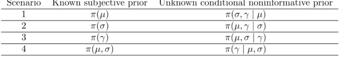
may be different for the different choices of{a(γ), b(γ)}. Nonetheless, a uniform prior of γwithin an appropriate interval could be a good choice as a subjective marginal prior onγ. We summarize these scenarios in Table 2.1:
Scenario Known subjective prior Unknown conditional noninformative prior
1 π(µ) π(σ, γ|µ)
2 π(σ) π(µ, γ |σ)
3 π(γ) π(µ, σ|γ)
4 π(µ, σ) π(γ|µ, σ)
Table 2.1: Scenarios of the RPPI in two-piece location-scale models.
For the two-piece location-scale models, we have the following theorem (Proofs are provided in Section 2.6):
Theorem 1 Consider the two-piece location-scale models in (2.3).
(a) Assume that the subjective marginal priorπ(µ)is available. The RPPI of(µ, σ, γ)is given by
π1(µ, σ, γ) = π(µ)π(σ, γ|µ) ∝ π(µ) σ s 1 a(γ) +b(γ) b0(γ)2 b(γ) + a0(γ)2 a(γ) − a0(γ) +b0(γ) a(γ) +b(γ) 2 ;
(b) Assume that the subjective marginal priorπ(σ)is available. The RPPI of(µ, σ, γ)is given by
π2(µ, σ, γ) =π(σ)π(µ, γ|σ) ∝ π(σ) v u u t 2α1 a(γ)b(γ) α2+ 1 a(γ) +b(γ) b0(γ)2 b(γ) + a0(γ)2 a(γ) − a0(γ) +b0(γ) a(γ) +b(γ) 2 − 4α 2 3λ(γ)2 a(γ) +b(γ)2;
(c) Assume that the subjective marginal priorπ(γ)is available. The RPPI of(µ, σ, γ)is given by
π3(µ, σ, γ) = π(γ)π(µ, σ|γ)∝
π(γ) σ2 ;
(d) Assume that the subjective marginal priorπ(µ, σ)is available. The RPPI of (µ, σ, γ)is given
by π4(µ, σ, γ) = π(µ, σ)π(γ|µ, σ) ∝ π(µ, σ) s α2+ 1 a(γ) +b(γ) b0(γ)2 b(γ) + a0(γ)2 a(γ) − a0(γ) +b0(γ) a(γ) +b(γ) 2 .
The above four priors are closely related to several independence Jeffreys priors based on a particular group partition of parameters discussed in [48]. In fact, π1(µ, σ, γ) with π(µ) ∝1 is
the same as the independence Jeffreys prior when the parameters are grouped as {µ,(σ, γ)}, and it is also the same as the modified Jeffreys prior in [47] if a(γ)·b(γ) is constant; π2(µ, σ, γ) with
π(σ) ∝ 1/σ is the same as the independence Jeffreys prior when the parameters are grouped as
{σ,(µ, γ)}; π3(µ, σ, γ) with π(γ) ∝ s α2+1 a(γ)+b(γ) b0(γ)2 b(γ) + a0(γ)2 a(γ) − a0(γ)+b0(γ) a(γ)+b(γ) 2 or π4(µ, σ, γ) with
π(µ, σ) ∝ 1/σ2 is the same as the independence Jeffreys prior when the parameters are grouped
as {(µ, σ), γ}. In addition, the Jeffreys priorπJ(µ, σ, γ) is a special case of π3(µ, σ, γ) withπ(γ)∝
withπ(µ, σ)∝1/σ.
To further study the propriety of the corresponding posterior distributions under the priors in Theorem 1, we firstly provide a useful lemma, whose proof is similar to that of Theorem 6 in [47] and is thus omitted for simplicity.
Lemma 2 Lety= (y1,· · ·, yn)be a random sample from the population with the pdf in (2.3), where
f(·)is a scale mixture of normals, that is,f(·)could be written as
f(x) =
Z ∞
0
ω·φ(ωx)dP(ω), (2.5)
whereφ(·)is the standard normal pdf andP(ω)is the cumulative distribution function of any positive
random variable. Consider a prior of(µ, σ, γ),
π(µ, σ, γ)∝ 1
σdπ(µ)π(γ), (2.6)
where d≥1,π(µ) is any bounded prior forµ, and π(γ)>0 forγ ∈Γ. A necessary condition for
the propriety of the joint posterior distribution of (µ, σ, γ)under the prior in (2.6) for n≥2is
Z
Γ
a(γ)n+d−1
a(γ) +b(γ)nπ(γ)dγ <∞. (2.7)
In addition, the posterior distribution of (µ, σ, γ) is proper provided that all the observations are
different andπ(γ)is proper whend= 1.
For the three models we considered: the ALD, the-skew model, and the inverse scale factors model, we choose the subjective marginal priors that specified in Theorem 1 as follows,π(σ)∝1/σd, π(γ)∝1, and π(µ, σ)∝π(µ)/σd, whered≥1 andπ(µ) being any bounded prior forµ. Since the location parameterµ does not affect the propriety of the posterior distribution, there is no need to specify the prior forµ. We discuss the propriety of the corresponding posterior distributions under the RPPI for those three special cases.
2.3.1
Asymmetric Laplace distribution
The pdf of the ALD can be obtained from (2.3) by specifying{a(γ) = 1/γ, b(γ) = 1/(1−γ)} andf(·) being the standard Laplace distribution
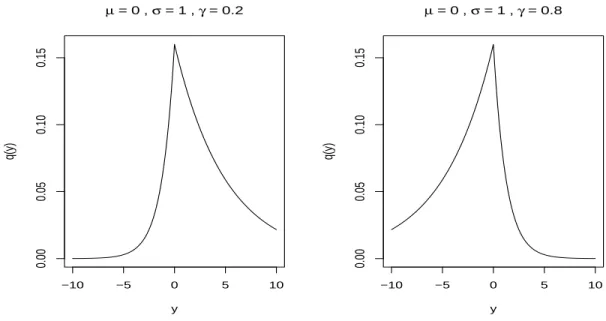
q(y|µ, σ, γ) = γ(1−γ) σ exp 1−γ σ (y−µ) , y≤µ, γ(1−γ) σ exp n −γσ(y−µ)o, y > µ, (2.8)
where−∞< µ <∞,σ >0, andγ is the skewness parameter whose value is between 0 and 1. The
ALD becomes the standard Laplace distribution when γ is equal to 0.5. It’s obviously to see that
the mode of the ALD isµ. The mean and variance of an asymmetric Laplace random variable are
given by E(y) = µ+ 1−2γ γ(1−γ)σ, V(y) = 1 γ2 + 1 (1−γ)2 σ2,
respectively. Note that the meanE(y) is greater than the mode µwhen γ is less than 0.5, which indicates that the density curve is skewed to the right. Similarly, the mean E(y) is less than the modeµwhenγ is greater than 0.5, so the density curve is skewed to the left. Two examples of the ALD could be seen from Figure 2.1.
It is easy to calculate thatα1= 1/2,α2= 1, and α3 = 1/2. Thus the Fisher information
matrix of the ALD is given by
IAL(µ, σ, γ) = γ(1−γ) σ2 0 − 1 σ 0 1 σ2 1 σ 2γ−1 γ(1−γ) −1 σ 1 σ 2γ−1 γ(1−γ) 1 γ2 + 1 (1−γ)2 ,
−10 −5 0 5 10 0.00 0.05 0.10 0.15 µ = 0 , σ = 1 , γ = 0.2 y q(y) −10 −5 0 5 10 0.00 0.05 0.10 0.15 µ = 0 , σ = 1 , γ = 0.8 y q(y)
Figure 2.1: Examples of the ALD
which yields the following RPPI
π1AL(µ, σ, γ) = π(µ)π(σ, γ|µ)∝ π(µ) σpγ(1−γ); π2AL(µ, σ, γ) = π(σ)π(µ, γ|σ)∝ 1 σd s 3γ2−3γ+ 1 γ(1−γ) ; π3AL(µ, σ, γ) = π(γ)π(µ, σ|γ)∝ 1 σ2; π4AL(µ, σ, γ) = π(µ, σ)π(γ|µ, σ)∝π(µ) σd s 1 γ2 + 1 (1−γ)2.
Corollary 1 Consider sampling from (2.3) withf(·)being the standard Laplace distribution,a(γ) =
1/γ, and b(γ) = 1/(1−γ) for γ ∈ (0,1). Then the posterior distribution is proper under prior
πAL
1 (µ, σ, γ)orπAL2 (µ, σ, γ)ifd= 1, and the posterior distribution is improper under priorπAL3 (µ, σ, γ)
orπAL
4 (µ, σ, γ).
Consider the RPPI for the ALD, the three marginal priors forγcorresponding toπAL
1 (µ, σ, γ), πAL 2 (µ, σ, γ) andπ4AL(µ, σ, γ) are π1AL(γ)∝ p 1 γ(1−γ), π AL 2 (γ)∝ s 3γ2−3γ+ 1 γ(1−γ) , and π AL 4 (γ)∝ s 1 γ2 + 1 (1−γ)2.
It is not difficult to verify that both πAL1 (γ) and π2AL(γ) are proper while πAL4 (γ) is improper.
Figure 2.2 displaysπAL
1 (γ), π2AL(γ), π4AL(γ) along with the uniform prior on (0,1) forγ, denoted by
πAL 3 (γ) for convenience. 0.0 0.2 0.4 0.6 0.8 1.0 0 1 2 3 4 5 γ Density π1 AL(γ) π2 AL(γ) π3 AL(γ) π4 AL(γ)
Figure 2.2: The marginal priors forγ
Corollary 1 states that among the four priors of (µ, σ, γ), bothπAL
1 (µ, σ, γ) andπAL2 (µ, σ, γ)
result in a valid Bayesian inference. More generally, we consider a general class of priors given by
π(µ, σ, γ)∝γ
s(1−γ)t
σh c(µ, σ, γ), (2.9)
whereh, s, t,∈R, andc(µ, σ, γ) is any positive and bounded function.
Theorem 2 Let y= (y1,· · ·, yn)be a random sample from the ALD.
(a) For the prior in (2.9), a sufficient condition for the posterior distribution to be proper is
h <min{s, t}+ 2 and n >max{−h+ 1,−min{s, t} −1}. (2.10)
(b) Ifc(µ, σ, γ)∝c1(µ), andc1(µ)is any positive and bounded function. The condition (2.10) for
[47] proposed an AG-Beta prior, which has form πAG(µ, σ, γ)∝ 1 σ |a0(γ)b(γ)−a(γ)b0(γ)| [a(γ) +b(γ)]α0+β0 a α0−1(γ)bβ0−1(γ),
where α0 and β0 are positive numbers. This prior is the same as the one π1(µ, σ, γ) if we choose
α0=β0= 1/2 andπ(µ)∝1. Moreover, for the ALD, we could simplify the AG-Beta prior as
πAGALD(µ, σ, γ)∝γ
β0−1(1−γ)α0−1
σ ,
which is a special case of our prior in (2.9). The AG-Beta prior has restrictions that α0 > 0 and
β0 >0, however, the prior in (2.9) is applicable to more general cases, s, t, and h can be any real
numbers as long as they satisfy the condition (2.10).
2.3.2
The
-skew model
The-skew model corresponds to (2.3) by specifying a(γ) = 1−γ and b(γ) =a+γ with γ∈(−1,1). A special case of the-skew model, the-normal density has been extensively discussed by [39]. A crucial idea in [39] is to form a distribution by joining at x= 0 two half normals with different scale parameters. [5] extended this idea to a more general family of distributions, the
-skew model, and then discussed the moment estimation of the -skew model and the asymptotic
normality of these estimates. Here we study this model from a Bayesian view. The Fisher information matrix of the-skew model is given by
I(µ, σ, γ) = 2α1 σ2(1−γ2) 0 − 2α3 σ(1−γ2) 0 α2 σ2 0 − 2α3 σ(1−γ2) 0 α2+1 1−γ2 .
the posterior distributions according to Theorem 1 and Lemma 2 π1(µ, σ, γ) = π(µ)π(σ, γ|µ)∝ π(µ) σp1−γ2; π2(µ, σ, γ) = π(σ)π(µ, γ|σ)∝ 1 σd(1−γ2); π3(µ, σ, γ) = π(γ)π(µ, σ|γ)∝ 1 σ2; π4(µ, σ, γ) = π(µ, σ)π(γ|µ, σ)∝ π(µ) σdp 1−γ2.
Corollary 2 Consider sampling from (2.3) withf(·)being a scale mixture of normals and{a(γ), b(γ)}
as in the-skew model. Then the posterior distribution is proper under priorπ
1(µ, σ, γ)orπ4(µ, σ, γ)
if d= 1, and the posterior distribution is improper under priorπ
2(µ, σ, γ).
Note that the propriety of the posterior distribution under priorπ3(µ, σ, γ) depends on the choice of
f(·). We can see that the posterior distribution is proper provided thatf(|x|) is decreasing in|x|. For example, f(·) can be a pdf of normal distribution, the Laplace distribution or any other scale mixture of normals.
2.3.3
The inverse scale factors model
The inverse scale factors model corresponds to (2.3) by specifyinga(γ) =γandb(γ) = 1/γ withγ >0. This model was firstly proposed by [18] through transforming an unimodal symmetric distribution. Bayesian inference for a regression analysis under the skewed-t distribution obtained from this class is also considered there. We study this model through the RPPI.
The Fisher information matrix of the inverse scale factors model is given by
IIS(µ, σ, γ) = 2α1 σ2 0 4α3 σ(1+γ2) 0 α2 σ2 α2(γ2−1) σ(γ+γ3) 4α3 σ(1+γ2) α2(γ2−1) σ(γ+γ3) α2 γ2 + 4 (1+γ2)2 ,
which yield the following RPPI πIS1 (µ, σ, γ) = π(µ)π(σ, γ|µ)∝ π(µ) σ(1 +γ2); πIS2 (µ, σ, γ) = π(σ)π(µ, γ|σ)∝ 1 σdγ(γ2+ 1) s (γ2+ 1)2 2 +γ 2 2−4 π ; πIS3 (µ, σ, γ) = π(γ)π(µ, σ|γ)∝ 1 σ2; πIS4 (µ, σ, γ) = π(µ, σ)π(γ|µ, σ)∝ π(µ) σd s α2 γ2 + 4 (γ2+ 1)2.
Corollary 3 Consider sampling from (2.3) withf(·)being a scale mixture of normals and{a(γ), b(γ)}
as in the inverse scale factors model, then the posterior distribution is proper under priorπ1IS(µ, σ, γ),
and the posterior distribution is improper under priorπ3IS(µ, σ, γ)orπIS4 (µ, σ, γ).
The propriety of the posterior distribution under prior πIS
2 (µ, σ, γ) heavily relies on the choice of
f(·). For example, the posterior distribution is improper whenf(·) is the standard normal density.
2.3.4
Inference on the asymmetric Laplace disrtribution
Now we focus on the posterior simulation when the ALD is considered. The RPPI are closely related to several independence Jeffreys priors, in order to distinguish them from the independence Jeffreys priors and highlight the subjective property that the RPPI possess, we advocate a different marginal prior for µ given by π(µ) ∝ exp{−(φ1(µ−φ2)2)/2} with φ1 ≥ 0 and φ2 ∈ R, due to
the conjugacy property. In this chapter, we employ an efficient Gibbs sampler for the posterior simulation. As an illustration, we only consider the case forπAL
1 (µ, σ, γ). We observe from Theorem
1 that π1AL(µ, σ, γ)∝ 1 σpγ(1−γ)exp −φ1(µ−φ2) 2 2 . (2.11)
Note that a mixture representation of the ALD could help us develop an efficient algorithm for the posterior simulation. Let z be a random variable following the ALD(µ, σ, γ). From [32], the
pdf ofzcould be reexpressed as z|µ, σ, γ, v ∼ N µ+av, bσv , (2.12) v|µ, σ, γ ∼ exp 1 σ , (2.13)
witha= (1−2γ)/(γ(1−γ)),b= 2/(γ(1−γ)), and exp(1/σ) stands for the exponential distribution with rate 1/σ. If we multiply the conditional density of z and v in (2.12) and (2.13), then the integration of the joint density with respect tovgives us the density of ALD in (2.8).
The ALD has various mixture forms due to different reparameteraztions. For example, [56] used three parameters (µ∗, σ∗, p) to describe the ALD, a one-to-one transformationµ=µ∗,σ=σ∗/2,
and γ=p∗ gives us the ALD in (2.8). The ALD in [56] can also be written as a scale mixture of
normals with the scale mixing parameter following an exponential distribution. [57] discussed four-parameter ALD(µ∗∗, σ∗∗, p1, p2). If we letµ=µ∗∗, σ=σ∗∗,γ =p1, andp1+p2 = 1, we have the
three-parameter ALD(µ, σ, γ) in (2.8). The four-parameter ALD(µ∗∗, σ∗∗, p1, p2) can be written as
a scale mixture of uniform with the scale mixing parameter following a Gamma distribution. Based on the mixture representation (2.12) and (2.13), the complete likelihood function of
ybecomes L(y|µ, σ, γ,v) ∝ n Y i=1 1 √ 2πbσvi ·exp −(yi−µ−avi) 2 2bσvi ∝ σ−n2γ n 2(1−γ) n 2 exp ( − n X i=1 (yi−µ−avi)2 2bσvi ) · n Y i=1 v−12 i , (2.14)
wherev= (v1, v2,· · · , vn), andvk∼exp(1/σ),k= 1,2,· · · , n. Note that the likelihood function in (2.14) involves the latent variablev, which can be viewed as a usual parameter in Bayesian analysis. Combining the complete likelihood function in (2.14) with the prior ofvin (2.13), and the prior of (µ, σ, γ) in (2.11), the joint posterior distribution of (µ, σ, γ,v) becomes
π(µ, σ, γ,v|y) ∝ L(y|µ, σ, γ,v)π(v|µ, σ, γ)π1AL(µ, σ, γ) ∝ σ −3n 2 −1 γ1−2n(1−γ) 1−n 2 ·exp ( − n X i=1 (yi−µ−avi)2 2bσvi −φ1(µ−φ2) 2 2 ) × exp ( − n X i=1 vi σ ) n Y i=1 v−12 i .
This yields the following full conditional posterior distributions vk|µ, σ, γ,y ∝ exp −(yk−µ−avk) 2 2bσvk ·expn−vk σ o ·v−12 k , k= 1, . . . , n; µ|σ, γ,v,y ∝ exp ( − n X i=1 (yi−µ−avi)2 2bσvi −φ1(µ−φ2) 2 2 ) ; σ|µ, γ,v,y ∝ σ−3n2−1exp ( − n X i=1 (yi−µ−avi)2 2bσvi ) ·exp ( − n X i=1 vi σ ) ; γ|µ, σ,v,y ∝ γn−21(1−γ) n−1 2 ·exp ( − n X i=1 (yi−µ−avi)2 2bσvi ) . (2.15)
Therefore, an efficient Gibbs sampler algorithm can be developed as follows. (i) Simulatevk from the inverse Gaussian distribution, IG(ak, bk) with
ak= s a2+ 2b (yk−µ)2 and bk = a2+ 2b bσ , k= 1,· · ·, n,
where the probability density function of IG(a, b) is given by
f(x|a, b) = r b 2πx −3 2exp −b(x−a) 2 2a2x , x >0.
(ii) Simulateµfrom the normal distribution, N(µ0, σ02) with
µ0= Pn i=1 yi vi−na+φ1φ2bσ Pn i=1 1 vi +φ1bσ andσ20= Pn bσ i=1 1 vi +φ1bσ .
(iii) Simulateσfrom the inverse Gamma distribution, Inverse-Gamma(3n/2, c1) with
c1= n X i=1 vi+ n X i=1 (yi−µ−avi)2 2bvi .
(iv) Simulateγ from the conditional posterior distribution in (2.15).
Although the full conditional posterior distribution of γ is not of standard form, we could employ the Metropolis-Hastings (M-H) method ([13]) for the posterior simulation from (2.15). The proposed Metropolis-within-Gibbs algorithm is commonly used in many literature, such as [56]. The difference is that [56] used the estimates as the mean and variance of the proposal density in the
M-H algorithm, whereas we use a random walk proposal M-H algorithm. Our simulation studies in the next section show that the proposed sampling algorithm is quite efficient in terms of mixing and convergence.
2.4
Simulation study and real data analysis
In this section, we carry out both Monte Carlo simulations and real data analysis to compare the performance of the proposed method with that of the MLEs. In the Metropolis step, we use a normal proposal to generate the samples.
2.4.1
Simulation study
The data in simulation studies are generated from the ALD in (2.8). We generate datasets for each of sample size n ={50,100,250,500}, and µ= 0, σ = 1, and γ ={0.2,0.3,0.5,0.7,0.8}, respectively. The distribution in (2.8) with various values ofγcovers the normal Laplace distribution (γ= 0.5) and some extreme situations (γ= 0.2 or 0.8). Moreover, in order to emphasize the case in which we have prior information of µ, we letφ1 = 1, andφ2 = 0 in (2.11). In other words, the
subjective marginal prior ofµis the standard normal distribution.
As stated by [45], a good acceptance rate in the Metropolis step is between 0.15 and 0.5 because high acceptance rates indicate that the sampler is not moving around the parameter space reasonably well, while low acceptance rates may indicate a slow mixing of the chain. Thus we check the acceptance rate for each dataset and only use the ones with good acceptance rates. We record 1,000 samples for each sample size and each choice ofγ.
Using a Markov chain Monte Carlo algorithm, a sample of size 40,000 was recorded from the posterior distribution after a burn-in period of 50,000 draws with a thinning of 10 draws. Based on the run length control diagnostic in [43], there is no evidence of lack of convergence. The Bayesian estimates were calculated by taking the average of the 1,000 repetitions. We here report the posterior mean and the posterior median, although other estimates may be used when an appropriate loss function is considered.
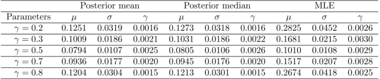
Table 2.2 compares the mean squared error (MSE) of Bayesian estimates and the one of
the maximum likelihood estimates (MLE) for all three parametersµ,σ, andγ whenn= 100. Note
γis far away from 0.5. Similar results also were observed forn= 50,250 and 500. As expected, the differences between these estimators become smaller as the sample size increases.
Posterior mean Posterior median MLE
Parameters µ σ γ µ σ γ µ σ γ γ= 0.2 0.1251 0.0319 0.0016 0.1273 0.0318 0.0016 0.2825 0.0452 0.0026 γ= 0.3 0.1009 0.0186 0.0021 0.1031 0.0186 0.0022 0.1681 0.0215 0.0030 γ= 0.5 0.0794 0.0107 0.0025 0.0805 0.0106 0.0026 0.1010 0.0108 0.0029 γ= 0.7 0.0936 0.0177 0.0020 0.0945 0.0176 0.0020 0.1517 0.0207 0.0028 γ= 0.8 0.1204 0.0304 0.0015 0.1213 0.0301 0.0015 0.2674 0.0418 0.0025
Table 2.2: MSEs of each parameter whenn= 100.
Table 2.3 provides the Bayesian estimates and MLEs along with their corresponding
stan-dard deviations. We observe that the MLE of µ overestimates the location parameter when γ is
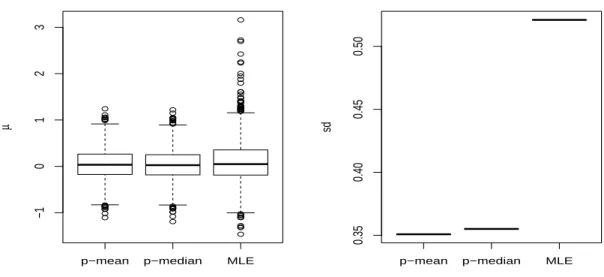
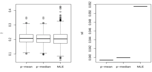
less than 0.5, and underestimates µ when γ is greater than 0.5, especially when γ is close to the endpoints of the interval (0,1), whereas the Bayesian approach offers better results, not only forµ, but also forσandγ. Moreover, the standard deviations for the Bayesian estimates are much smaller than the ones of the MLEs. Figure 2.3 - 2.5 provide a more straight forward comparison of two approaches on point estimation and the corresponding standard deviations.
Table 2.4 displays the acceptance rate for the Metropolis step when sample size is 100. Note that all rates are located in the interval [0.15, 0.5] which indicates that the proposed method is efficient. In addition, Table 2.5 gives the frequentist coverage probabilities of 95% credible intervals for the three parameters. Note that the coverage probabilities are very close to 0.95 for all the three parameters. Therefore, the Bayesian estimates have good frequentist properties. The phenomenon when sample size is not 100 is quite similar, thus, the results where the sample size is different are
Posterior mean Posterior median MLE
Parameters µ σ γ µ σ γ µ σ γ γ= 0.2 0.0470 1.0319 0.2086 0.0386 1.0202 0.2061 0.1068 0.9952 0.2056 (0.3507) (0.1759) (0.0393) (0.3550) (0.1772) (0.0399) (0.5209) (0.2128) (0.0515) γ= 0.3 0.0372 1.0035 0.3043 0.0344 0.9965 0.3027 0.0802 0.9795 0.3037 (0.3156) (0.1367) (0.0467) (0.3195) (0.1364) (0.0472) (0.4023) (0.1454) (0.0547) γ= 0.5 0.0057 1.0051 0.5011 0.0048 0.9985 0.5011 0.0049 0.9842 0.5011 (0.2819) (0.1038) (0.0505) (0.2839) (0.1031) (0.0510) (0.3180) (0.1030) (0.0543) γ= 0.7 -0.0138 1.0054 0.6952 -0.0101 0.9982 0.6968 -0.0529 0.9806 0.6961 (0.3058) (0.1332) (0.0449) (0.3075) (0.1330) (0.0454) (0.3861) (0.1429) (0.0533) γ= 0.8 -0.0574 1.0305 0.7903 -0.0502 1.0192 0.7927 -0.1342 1.0009 0.7916 (0.3424) (0.1719) (0.0380) (0.3448) (0.1726) (0.0384) (0.4996) (0.2046) (0.0493) Table 2.3: Bayesian estimates and MLEs with corresponding standard deviations (sd) in parenthesis when sample size is 100.
p−mean p−median MLE −1 0 1 2 3 µ
p−mean p−median MLE
0.35
0.40
0.45
0.50
sd
Figure 2.3: Boxplots summarizing the Bayesian estimates and MLE of µ, and the corresponding
standard deviations whenγ= 0.2 and sample size is 100.
p−mean p−median MLE
0.4 0.6 0.8 1.0 1.2 1.4 1.6 σ
p−mean p−median MLE
0.18
0.19
0.20
0.21
sd
Figure 2.4: Boxplots summarizing the Bayesian estimates and MLE of σ, and the corresponding
p−mean p−median MLE 0.1 0.2 0.3 0.4 γ
p−mean p−median MLE
0.040 0.042 0.044 0.046 0.048 0.050 0.052 sd
Figure 2.5: Boxplots summarizing the Bayesian estimates and MLE of γ, and the corresponding
standard deviations of them whenγ= 0.2 and sample size is 100.
omitted here for simplicity.
Parameters acceptance rate
γ= 0.2 0.1672
γ= 0.3 0.2718
γ= 0.5 0.3771
γ= 0.7 0.2659
γ= 0.8 0.1734
Table 2.4: Acceptance rates for the Metropolis step when n=100.
2.4.2
Real data analysis
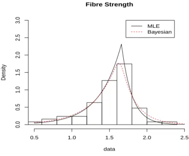
We consider the fibre strength data. The samples are the experimental data of the strength
of n= 63 glass of fibre of length 1.5 cm, from the National Physical Laboratory in England. The
data set was provided by [50]. We fit the data by applying the asymmetric Laplace distribution. The MLEs of (µ, σ, γ) are given by (1.6600, 0.0943, 0.6774). As stated in Corollary 1, the posterior distribution is proper when a normal prior forµis considered. Thus we choose the normal distribution N(1.6,1) as our subjective prior for µ whose prior mean is close to the MLE of µ. According to Theorem 1, the RPPI of (µ, σ, γ) isπ(µ, σ, γ)∝1/(σpγ(1−γ)) exp{−(µ−1.6)2/2}.
n=100 Parameters µ σ γ γ= 0.2 0.965 0.961 0.964 γ= 0.3 0.969 0.953 0.960 γ= 0.5 0.971 0.951 0.958 γ= 0.7 0.962 0.950 0.956 γ= 0.8 0.972 0.956 0.960
Table 2.5: Frequentist converge probability of 95% CI.
Fibre Strength data Density 0.5 1.0 1.5 2.0 2.5 0.0 0.5 1.0 1.5 2.0 2.5 3.0 MLE Bayesian
Figure 2.6: Fitted curves and data histogram: Bayesian predictive density curve (Bayesian), and MLEs based curve (MLE).
The acceptance rate for Metropolis sampling is 0.40432 showing that the result is reasonable. The improvement of fitting is demonstrated in Figure 2.6, where the histogram of the data with the 0.2 cm bin-size is overlaid with Bayesian predictive density curve and fitted MLE curve. We observe that the predictive density curve reflects the data more precisely, especially at the mode of the data.
2.5
Concluding remarks
In this chapter, we have extensively studied Bayesian analysis for a special case of the two-piece location-scale models, the ALD. We have also proposed similar results other two sub-models,
partial information proposed in [52] and have shown that two of them lead to proper posterior distributions for the ALD. The RPPI are different from the independence Jeffreys prior in that they could include subjective prior information for some parameters. Specifically, we focus our discussion on the mostly widely used distribution, the ALD. Numerical results have shown that the proposed Bayesian estimates outperform the MLEs, especially when symmetry is not appropriate.
Since the seminal work of [27], quantile regression has gained increasing popularity in differ-ent areas of study as a comprehensive approach to the statistical analysis of linear response models. Due to the close relationship between the ALD and quantile regression discussed in [61], researchers conduct Bayesian analysis by imposing the ALD on the error terms in the classical linear regression model. Therefore, we plan to extend the proposed Bayesian approach to deal with the quantile regression. This work is currently under investigation and will be reported elsewhere.
2.6
Proofs
Proof of Theorem 1: We provide the proof for part (a) only because the proofs for other cases are quite similar. LetI22(σ, γ) denote the corresponding Fisher information submatrix of (σ, γ). It
can be seen from Remark 2 that
I22(σ, γ) = α2 σ2 α2 σ ha0(γ)+b0(γ) a(γ)+b(γ) i α2 σ ha0(γ)+b0(γ) a(γ)+b(γ) i α2+1 a(γ)+b(γ) hb0(γ)2 b(γ) + a0(γ)2 a(γ) i −haa0((γγ)+)+bb0((γγ))i2 .
Through Lemma 1, the conditional reference prior for (σ, γ) givenµis given by
π(σ, γ|µ) ∝ |I22(σ, γ)| ∝ 1 σ s 1 a(γ) +b(γ) b0(γ)2 b(γ) + a0(γ)2 a(γ) − a0(γ) +b0(γ) a(γ) +b(γ) 2 .
This yields the RPPI of (µ, σ, γ)
π(µ, σ, γ)∝ π(µ) σ s 1 a(γ) +b(γ) b0(γ)2 b(γ) + a0(γ)2 a(γ) − a0(γ) +b0(γ) a(γ) +b(γ) 2 .
Proof of Theorem 2: Given datay= (y1, y2,· · ·, yn), and the prior π(µ, σ, γ) in (2.9), the pos-terior distribution of (µ, σ, γ) becomes
π(µ, σ, γ |y)∝c(µ, σ, γ)γ s(1−γ)t σh γn(1−γ)n σn n Y i=1 exp −yi−µ σ (γ−I(yi≤µ)) .
Note that the above posterior distribution is proper if and only if
Z 1 0 Z ∞ −∞ Z ∞ 0 c(µ, σ, γ)γ n+s(1−γ)n+t σn+h n Y i=1 exp −yi−µ σ (γ−I(yi≤µ)) dσdµdγ <∞.
(a) Sincec(µ, σ, γ) is a positive and bounded function, there exists a positive number B such that c(µ, σ, γ)< B. Therefore, we obtain an upper bound for the left side of the above inequality
B· Z 1 0 Z ∞ −∞ Z ∞ 0 γn+s(1−γ)n+t σn+h n Y i=1 exp −yi−µ σ (γ−I(yi≤µ)) dσdµdγ.
After integrating outσ, the above formula is finite if and only if
Z 1 0 γn+s(1−γ)n+t Z ∞ −∞ 1 P(y i−µ)(γ−I(yi ≤µ)) n+h−1 dµdγ <∞.
Assume (y(1), y(2),· · ·, y(n)) is the order statistics ofy. For each interval (y(i), y(i+1)), we have
Z y(i+1) y(i) 1 n P k=1 (yk−µ)(γ−I(yk ≤µ)) n+h−1 dµ ≤ Z y(i+1) y(i) 1 n P k=i+1 (y(k)−µ)γ n+h−1 dµ = 1 γn+h−1Ai,
hold for the intervals (−∞, y(1)) and (y(n),∞), Z y(1) −∞ 1 Pn k=1(yk−µ)(γ−I(yk≤µ)) n+h−1 dµ = 1 γn+h−1A0, Z ∞ y(n) 1 Pn k=1(yk−µ)(γ−I(yk≤µ)) n+h−1 dµ = 1 (1−γ)n+h−1An, where A0= [Pn k=1yk−ny(1)]−(n+h)+2 (−(n+h)+2)(−n) andAn = [ny(n)−Pnk=1yk]−(n+h)+2 (−(n+h)+2)(−n) .
Combining the above results, we have
Z 1 0 Z ∞ −∞ Z ∞ 0 π(µ, σ, γ|y)dσdµdγ < B Z 1 0 γn+s(1−γ)n+t " 1 γn+h−1 n−1 X i=0 Ai+ 1 (1−γ)n+h−1An # dγ = n−1 X i=0 AiB Z 1 0 γs−h+1(1−γ)n+tdγ+AnB Z 1 0 γn+s(1−γ)t−h+1dγ.
Note that the first term is finite if and only ifs−h+ 1>−1 andt+n >−1, and the second term is finite if and only ift−h+ 1>−1 ands+n >−1. Therefore, we obtain a sufficient condition for the posterior distribution to be proper,
h <min{s, t}+ 2 and n >max{−h+ 1,−min{s, t} −1}.
(b) Ifc(µ, σ, γ)∝c1(µ), then the prior for (µ, σ, γ) becomes
π(µ, σ, γ)∝ γ
s(1−γ)t σh c1(µ).
The necessary part is just the direct application of Lemma 2. Therefore, the condition (2.10) is necessary and sufficient for the posterior distribution to be proper.
Chapter 3
Variable Selection in Quantile
Regression
3.1
Quantile regression
Consider a simple decision theoretic problem: a point estimate is required for a random variable X with distribution functionF(·). Given the loss function is
ργ(µ) =µ(γ−I(µ <0)), (3.1)
whereγis a number between 0 and 1, we want to find the ˆxthat minimizes the expected loss which is given by E[ργ(X−xˆ)] = (γ−1) Z xˆ −∞ (x−xˆ)dF(x) +γ Z ∞ ˆ x (x−xˆ)dF(x). (3.2)
Differentiate both sides with respect to x, we have
0 = (1−γ) Z xˆ −∞ dF(x)−γ Z ∞ ˆ x dF(x) =F(ˆx)−γ.
Thus any element of {x: F(x) = γ} minimizes the expected loss. If the solution is unique, then ˆ
the smallest one. Thus theγth quantile of X is defined by ([27])
F−1(γ) = inf{x:F(x)≥γ}.
IfF(·) is replaced by the empirical distribution function
Fn(x) =
Pn
i=1I(xi≤x)
n ,
where (x1, x2,· · ·, xn) is a random sample. We still choose ˆxto minimize the expect loss (3.2)
Z
ργ(x−xˆ)dFn(x) =
Pn
i=1ργ(xi−xˆ)
n ,
the resulting estimate is the γth sample quantile. Therefore, the problem of finding γth sample quantile becomes a minimization problem
min x n X i=1 ργ(xi−x).
[27] employed this idea and proposed the quantile regression. Consider the linear model
yi=xTiβ+εi, (3.3)
wherey= (y1, y2,· · ·, yn)T is the response vector,xi= (xi1, xi2,· · · , xip)T represents the p known covariates, fori= 1,2,· · · , n, β= (β1, β2,· · · , βp)T is a p×1 vector of the regression coefficients, and εi’s are independent error terms whose distribution is unknown, but is restricted to have the γth quantile equal to zero. Thus theγth regression quantile is defined as any solution β(γ) to the
quantile minimization problem
min β n X i=1 ργ(yi−xTiβ). (3.4)
Compared with the linear mean regression, quantile regression has two advantages. First, it provides richer information in the effects of the predictors on the different quantiles of the re-sponse variable than the one under the regular mean regression. Second, it is very insensitive to heteroscedasticity and outliers, thus quantile regression can accommodate non-normal errors, which
are commonly encountered in many practical applications. These two appealing features of quantile regression result in its broader application in a wide range of disciplines, see [23], [28], [55].
Variable selection plays an important role in the model building process to obtain a bet-ter inbet-terpretation and to improve the precision of model fit. The problem of variable selection is equivalent to identifying an appropriate subset of important variables via the regression coefficients. Over the years, numerous procedures have been developed for the variable selection in the quantile regression models. In Section 3.2, we review some frequentist variable selection methods in the quantile regression. Bayesian variable selection methods in the quantile regression are reviewed in Section 3.3. In Section 3.4, we discuss a drawback in the existing methods and the way how we handle it.
3.2
Frequentist variable selection in the quantile regression
Frequentists usually adopt regularization methods for the variable selection in the quantile regression by automatically setting several coefficient estimates to zeros, such as the Lasso ([37]), SCAD ([58]), adaptive Lasso([58]), to name just a few.
3.2.1
The Lasso
Consider the usual linear regression situation, the ordinary least squares (OLS) estimates are obtained by minimizing the residual squared error. The OLS estimates have two drawbacks. First, it often have low bias but large variance which would decrease prediction accuracy. Second, with a large number of predictors, we desire to choose a small subset which provides the strongest effects rather than estimating the whole model. Two techniques, ridge regression and subset selection, have been proposed to improve the OLS estimates. However, both two techniques have some drawbacks, too. The ridge regression increases the stability of the model by shrinking the coefficients, but it does not set any coefficients to 0 and thus could not provide an easy interpretable model. Subset selection provides interpretable models, but it is sensitive to the data since it is a discrete process, thus small changes in the data can result in quite different models and the prediction accuracy will be reduced.
Motivated by those facts, [53] proposed the Lasso method which not only shrinks the co-efficients and set others to 0, but also remains the good properties of ridge regression and subset
selection. Consider the linear model
yi=xTiβ+εi, (3.5)
wherey= (y1, y2,· · ·, yn)T is the response vector,xi= (xi1, xi2,· · · , xip)T represents the p known covariates, fori= 1,2,· · · , n, β= (β1, β2,· · · , βp)T is a p×1 vector of the regression coefficients, and εi’s are independent identically distributed normal errors with mean 0 and unknown variance σ2. The Lasso estimates are defined as
ˆ β= arg min β ( n X i=1 (yi−xTiβ)2 ) subject to p X j=1 |βj| ≤t, (3.6)
for some non-negative number t, and (3.6) is equivalent to the minimization problem
min β n X i=1 (yi−xTiβ) 2+λ p X j=1 |βj| , (3.7) whereλ≥0.
We consider the check function (3.1) as our loss function in the quantile regression model (3.3), the Lasso estimates of the quantile regression are given by ([37])
min β ( n X i=1 ργ(yi−β0−xTiβ) ) (3.8) subject to p X j=1 |βj| ≤s, (3.9)
where s is the regularization parameter. We refer to it as L1-norm quantile regression (L1-norm
QR). The above minimization problem could be rewritten as
min β0,β γ n X i=1 ξi+ (1−γ) n X i=1 ζi, subject to p X j=1 |βj| ≤s, −ζi≤yi−f(xi)≤ξi, ζi, ξi ≥0, i= 1, . . . , n,
wheref(xi) =β0+P
p
j=1βjxij. [37] derived the Lagrangian primal function to compute the solution path{β(s),0 ≤s≤ ∞} Lp: γ n X i=1 ξi+ (1−γ) n X i=1 ζi+λ? p X j=1 |βj| −s + n X i=1 αi(yi−f(xi)−ξi) − n X i=1 δi(yi−f(xi) +ζi)− n X i=1 κiξi− n X i=1 ηiζi, whereλ?, α
i, δi, κi andηi are non-negative Lagrangian multipliers. Letθi =αi−δi, and we define the elbow set as
Φ={i:yi−f(xi) = 0,−(1−γ)≤θi≤γ}.
As s increases, an event is defined to be either a residualyi−f(xi) changes from nonzero to zero or a coefficientβj changes from nonzero to zero. Thus points inΦstay in the elbow set unless an event happens. Therefore, nonzeroβj’s satisfy:
yi−(β0+
X
j∈Ψ
βjxij) = 0 for i∈Φ,
where Ψ ={j : βj 6= 0}. The idea of the algorithm proposed by [37] is: we start withs = 0 and increase it, and keep track of the location of all data points relative to the elbow set and also of the magnitude of the fitted coefficients along the way. As s increases, if a point passes throughΦ, the correspondingθi must change fromγ to−(1−γ) or vice versa, thus points inΦmust linger in the elbow set. Since all points in the elbow set satisfyyi−f(xi) = 0, a path forβcan be established.
The algorithm focuses on the set of points Φ and the set of nonzero coefficients Ψ. Let βl
0,β
l and sl be the parameter values, Ψl be the set of nonzero coefficients, fl(·) be the function
immediately after thelth event. As shown by [37],
β0 = β0l+ (s−s l)v 0, (3.10) βj = βjl+ (s−s l )vj, ∀j ∈Ψl, (3.11) f(x) = (s−sl) v0+ X j∈Ψl vjxj +fl(x), (3.12)
where v0 = (β0−β0l)/(s−sl) and vj = (βj −βjl)/(s−s
l). Note that from equations (3.10) and (3.11),β0andβj proceed linearly in s forsl< s < sl+1, and equations (3.11) and (3.12) provide us a way to computesl+1. We compute the rate of change of the loss function to update setsΦandΨ
when thelth event occurs:
4loss 4s = Pn i=1ργ(yi−f(xi))−P n i=1ργ(yi−fl(xi)) s−sl = (1−γ)X i∈L v0+ X j∈Ψ vjxij −γ X i∈R v0+ X j∈Ψ vjxij ,
whereL={i:yi−f(xi)<0, θi=−(1−γ)}andR={i:yi−f(xi)>0, θi=γ}. By the definition of an event, there will be|Ψ|variables with nonzero coefficients and|Ψ|+ 1 points in the elbow set,
we need to either remove a point in Φfrom Φ, or add a variable not inΨinto Ψ. We choose the
update that corresponds to the smallest4loss/4s, and terminate the algorithm when all4loss/4s are non-negative.
3.2.2
Smoothly clipped absolute deviation
In the framework of regularization, many different types of penalties have been introduced to achieve variable selection. A good penalty should have three desirable properties ([17]), i) the penalty functions have to singular at the origin to produce sparse solutions; ii) they have to be bounded by a constant to produce nearly unbiased estimates for large coefficients; and iii) they have to ensure the stability of model selection. The Lasso method we discussed in Section 3.2.1 uses theL1 penalty, it creates large bias for coefficients ([17]) and thus L1 penalty may not be a good
penalty. As an alternative way, [17] proposed an approach by choosing new penalty functions who
are symmetric and convex on (0,∞), the smoothly clipped absolute deviation (SCAD) function is
one of those penalty functions.
Later on, [58] studied the penalized quantile regression with the SCAD penalty. The SCAD penalty is defined in terms of its first derivative and is symmetric around the origin. Forθ >0, its first derivative is p0λ(θ) =λ I(θ≤λ) +(aλ−θ)+ (a−1)λ I(θ > λ) , (3.13)
wherea >2 andλ >0 are tuning parameters. Consider the model (3.3) and the loss function (3.1), the SCAD penalized quantile regression solves the minimization problem ([58])
min β n X i=1 ργ(yi−xTiβ) +n p X j=1 pλn(|βj|). (3.14)
Note that the first derivative of the SCAD penalty function (3.13) can be viewed as a sum of two functions: one constant term and the other with a decreasing function on the range (0,∞). Therefore, the SCAD penalty function can be decomposed as the difference of two convex functions
pλ(θ) =pλ,1(θ)−pλ,2(θ), (3.15)
where bothpλ,1(·) andpλ,2(·) are convex functions with derivatives given by
p0λ,1(θ) = λ, p0λ,2(θ) = λ 1−(aλ−θ)+ (a−1)λ I(θ > λ), for θ >0.
Based on this decomposition, the Difference Convex Algorithm (DCA) ([3]) can be used to solve the minimization problem (3.14). The DCA minimizes a non-convex objective function by solving a sequence of convex minimization problems. At each iteration, it approximates the second convex function by a linear function. Then the objective function at each step is convex and easier to optimize than the original one. For the quantile regression, the resulting optimization at each iteration is a linear programming which indicates that the algorithm is very efficient.
According to the decomposition (3.15), the objective function in (3.14) can be decomposed asQvex(β) +Qcav(β), where
Qvex(β) = n X i=1 ργ(yi−xTi β) +n p X j=1 pλn,1(|βj|), Qcav(β) = −n p X j=1 pλn,2(|βj|).
Letβ(t)= (β1(t), β2(t),· · · , βp(t))T be the solution at step t. As proposed by [58], the algorithm
that minimizesQvex(β) +Qcav(β) is as follows