ON ESTIMATING QUANTILES USING AUXILIARY INFORMATION
Berger, Y.G and Mu˜noz, J.F. Abstract
We propose a novel approach for estimating quantiles using auxiliary information. The proposed estimator can be easily implemented using the regression estimator. The proposed approach does not require joint-inclusion probabilities and does not assume that the auxiliary variable is known at the population level. We show that the proposed estimator is consistent and asymptotically unbiased. The main advantage of the pro-posed estimator is its simplicity. Despite the fact the propro-posed estimator is not necessarily more efficient than its competitors, it offers a good com-promise between accuracy and simplicity. It can be used under single and multi-stage sampling designs with unequal selection probabilities. A simulation study supports our finding and shows that the proposed esti-mator is robust and of an acceptable accuracy compared to alternative estimators, which are more computationally intensive.
Key works: Regression Estimator; Distribution Function; Normal Distribution; Sample Survey
1
Introduction
Estimation of quantiles may be of considerable interest when measuring income distribution and poverty lines [e.g. Osier (2009), Verma and Betti (2011), Eurostat (2003), Berger and Skinner (2003)]. For instance, the median is regarded as a more appropriate measure of location than the mean when the variables, such as income, expenditure, etc, have highly skewed distributions.
In addition, quantile estimation is a topic of relevant importance in many practical applications [Law and Kelton (1991), Cannamela et al. (2008)]. In sample surveys, auxiliary information is often used at the estimation stage
to improve the estimation of target parameters. In particular, the use of auxiliary information has been studied extensively for estimation of means. However, it has no obvious extensions to the estimation of quantiles. In this paper, we propose a novel estimator for quantiles which takes into account of
the auxiliary information.
We consider a finite populationU ={1, . . . , i, . . . , N}containingN units. Let
y1, . . . , yN denote the values of the variable of interest,y, andx1, . . . , xN denote the values of an auxiliary variable,x. A samples, of sizen, is selected fromU according to a sampling design. The aim is to estimate the population
quantile
Yα=F−1(α), (1) where F(t) =N−1P
i∈Uδ(yi≤t) is the population distribution function and
δ(·) is the indicator function which takes the value 1 if its argument is true and 0 otherwise. The functionF−1(·) is the inverse of the functionF(·).
Throughout this paper, we define the inverse of any functionG(·) by
G−1(α) = inf{t:G(t)≥α}.
A customary estimator forYαis obtained by substitutingF(t) by its estimator into (1). For example, the H´ajek type estimator ofYαis defined by
b Yπ;α=Fbπ−1(α), (2) with b Fπ(t) = 1 b N X i∈s δ(yi≤t) πi (3)
andNb =Pi∈sπ−i1, whereπi denotes the first-order inclusion probability of uniti. There exists a wide range of estimators for the distribution function
The proposed estimator is based upon a transformation of the variable of interest. We show that the proposed estimator consists in substitutingαby
b
αreg into (2), where the quantityαbreg, defined in (16), takes the auxiliary information into account. The proposed estimator can be justified by using a
transformation of the variable of interest.
We propose a simple estimator which can be computed in situations where alternative estimators can not be obtained. For instance, the proposed method
can be used if we only know the calibration weights and the first order inclusion probabilities are unknown, whereas the Rao et al. (1990)’s estimator
can not be obtained in this situation. This is due to the fact that the Rao et al. (1990)’s estimator depends on the joint inclusion probabilities, which can be unknown for multi-stage designs. The proposed estimator can be naturally
used with multi-stage designs. A simulations study shows that the proposed estimator is good compromise in term of simplicity and efficiency. In Section 2, we define estimators of the distribution function that can be
found in the literature, and which can be used to estimate a quantile. In Section 3, we introduce the proposed estimator for a quantile. In Section 4, we give regularity conditions under which the proposed estimator is consistent. In
Section 5, we propose a simple approach to estimate the precision of the proposed estimator. In Section 6, we compare via simulation the proposed estimator with the alternative estimators defined in Section 2. This paper
concludes with some discussions in Section 7.
2
Estimators of quantiles
The model based estimator for the distribution function suggested by Chambers and Dunstan (1986) is based on the following heteroscedastic
regression model
whereβ is an unknown parameter,ν(xi) is a known function ofxand theui are independent and identically distributed random variables with zero mean.
The distribution function estimator proposed by Chambers and Dunstan (1986) is b Fcd(t) = X i∈s δ(yi≤t) +1 n X j∈U−s X i∈s δ uni≤t−bnxj ν(xj) , (5) with bn = " X i∈s x2 i ν2(xi) #−1 X i∈s yixi ν2(xi); uni= yi−bnxi ν(xi) . The Chambers and Dunstan (1986) estimator ofYαis given by
b
Ycd;α=Fbcd−1(α).
Rao et al. (1990) proposed the following estimator
b Frkm• (t) = 1 N ( X i∈s πi−1δ(yi≤t) + X i∈U b Gi(t)−X i∈s π−i 1Gbic(t) !) where b Gi(t) = 1 b N X j∈s 1 πj δ buj ≤ t−Rxb i x1i/2 ! , b Gic(t) = X j∈s πi πij −1 X j∈s πi πij δ buj ≤ t−Rxb i x1i/2 ! , b uj = yj−Rxb j x1j/2 , b R = " X i∈s xi πi #−1 yi πi ,
and where πij denotes the joint inclusion probability for the unitsiandj. Since the estimatorFb•
rkm(t) is not always a monotone non-decreasing function, Rao et al. (1990) proposed to use the following estimator
b
Frkm(t) = maxnFerkm(y(i)) :y(i)≤t
o
where they(i)’s are the order statistics of the sample{yi, i∈s}and Ferkm(y(i))
is defined by the following recursive formula
e Frkm(y(i)) = max n e Frkm(y(i−1)),Fbrkm• (y(i)) o
withFerkm(y(1)) =Fbrkm• (y(1)). The Rao et al. (1990) estimator ofYα is given byYbrkm;α=Fbrkm−1 (α).
Silva and Skinner (1995) proposed the following estimator based on post-stratification b Fps(t) = 1 N G X g=1 Ng b Ng X i∈s 1 πiδ(yi≤t)δ(i∈Ug), (7) whereU1, . . . , UG areGpost-strata partitioning the population,Ng is the size
ofUg andNbg=Pi∈sgπ
−1
i , withg= 1, . . . , G. The Silva and Skinner (1995) estimator ofYαis given byYbps;α=Fbps−1(α).
When the population quantileXα of an auxiliary variable is known, Rao et al. (1990) proposed the following ratio estimator ofYα
b Yr;α= b Yπ;α b Xπ;α Xα, (8)
whereYbπ;αandXbπ;α are respectively the H´ajek estimators ofYαand Xα[see (2)]. Rao et al. (1990) also proposed a difference estimator given by
b
Yπ;α+Rb(Xα−Xbπ;α) and showed thatYbr;α has a smaller mean square error than the difference estimator. Note that the estimatorsYbcd;α,Ybrkm;αandYbps;α assume that the auxiliary variable is known for all the units of the population,
whereas estimatorYbr;α only requires the knowledge ofXα. The estimator
b
Yrkm;α also requires the joint-inclusion probabilities.
3
Proposed estimator for a quantile
The proposed estimator is based upon the following idea, which can be illustrated for a median. If the distribution of the variable of interest is such
that the mean equals the median, the median could be estimated by using an estimator for the mean. We propose to transform the variable of interest in such a way that the median equals the mean for the transformed variable. If
the transformation is monotone increasing, the median of the variable of interest can be estimated by inverting the estimate for the mean of the transformed variable. This method can also be extended to the estimation of
any quantile.
The proposed estimator is given by (15) in Section 3.3. In order to justify this estimator, it is necessary to transform the variable (Section 3.1) and to use a
regression estimator (Section 3.2).
3.1
A transformation of the variables
We propose to transform the variable of interest in a way that the distribution of the transformed variable is approximately symmetric. Consider the
transformed values
y∗α;i= Ψ(yi) +zκ, (9) where Ψ(yi) =φ−1(F◦(yi)) andφ−1(·) is the quantile function of a normal
N(0,1) distribution or the inverse of the following cumulative distribution function φ(y) = 1 (2π)1/2 Z y −∞ exp −t2 2 dt.
The quantityzκis a known offset term which is given by theκ-th quantile of a normalN(0,1) distribution, whereκ= (dαNe −0.5)/N; that is,zκ=φ(κ). Note thatκcan be approximated byαfor large populations, asκ→αwhen
N → ∞. The functionF◦(·) is the mid-point distribution function [Nyg˚ard and Sandstr¨om (1985)] of the variable of interest defined by
F◦(y) =1
Note that 0< F◦(yi)<1 for alli∈U. We have to use (10) instead ofF(t) because the functionφ−1(·) is not defined on 0 and 1.
The following Lemma gives the relationship between the population quantile
Yα and the population mean of the transformed variable
Y∗α= 1 N X i∈U yα∗;i. Lemma 1. We have thatYα= Ψ−1(Y∗
α), where the function Ψ−1(·)is the
inverse of function Ψ(·)defined in (9). The proof is given in Appendix A.
The transformed values in (9) depend on population values, which would need to be estimated. We propose to estimatey∗
α;i by its substitution estimator given by
b
y∗α;i=Ψ(b yi) +zκ,
whereΨ(b yi) =φ−1(Fb◦(yi)). The functionFb◦(·) is an empirical mid-point estimator of the distribution function (10). This estimator is given by
b
F◦(y) =1
2[Fb(y )−Fb(y)], (11) whereFb(·) is one of the estimators of the distribution function defined previously. This function could be (3), (5), (6) or (7). For example, with the
Rao et al (1990) estimatorFb(t) =Fbrkm(t) and the mid-point distribution function is given byFb◦
rkm(y) = [Fbrkm(y )−Fbrkm(y)]/2. The Chambers and Dunstan (1986) and Silva and Skinner (1995) mid-point distribution function
can be defined in a similar way.
The auxiliary variable may be transformed in the same way. Consider
x∗α;i= Ψx(xi) +zκ,
where Ψx(xi) =φ−1(Fx◦(xi)),Fx◦(x) = [Fx(x)−Fx(x)]/2 and
Fx(t) = 1
N
X
i∈U
Note that the values ofx∗
α;i cannot be calculated if we only know the sampled values of the auxiliary variable, as the functionFx(·) is unknown in this
situation. If this is the case, we propose to estimateFx(·) by one of its estimators (see (3), (5), (6) or (7)).
3.2
The regression estimator
We propose to estimateY∗αusing the regression estimator [e.g. Cassel et al. (1976, 1977)], which uses the auxiliary information. This estimator is defined
by y∗reg;α=y∗α+βbx(X ∗ α−x∗α), (12) wherey∗ α=N−1 P i∈sπ −1 i byα∗;i,X ∗ α=N−1 P i∈Ux∗α;i,x∗α=N−1 P i∈sπ −1 i x∗α;i, with b βx= " X i∈s 1 πiqi2 (x∗α;i−x∗α)2 #−1 X i∈s 1 πiq2i (x∗α;i−x∗α)(yb∗α;i−y∗α). (13) Note that if we only know the sampled values of auxiliary variable, the control
meanX∗α can be estimated byXb ∗
α=Ψx(b Xα), as long as we know the population quantile Xαof the auxiliary variable.
Note that the regression estimatory∗
reg;α is based on the working regression model
b
yα∗;i=β0+βxx∗α;i+qii, (14) whereqi ∝(x∗α;i)γ, and i is a residual with mean 0.
Asφ−1(·) is the quantile function of a normal distribution, the distribution of
theyb∗
α;i’s and thex∗α;i’s is approximately normal. Normality is a desirable property that can improve the estimation of the regression parameters in (14).
For example, if the distribution of the variable of interest is normal given the auxiliary variable, the coefficient (13) is the maximum likelihood estimator.
3.3
The proposed estimator
Based on Lemma 1, the proposed estimator is given by
b
Yreg;α=Ψb−1(y∗reg;α). (15) AsΨb−1(y) =Fb◦−1(φ(y)), an alternative expression for the proposed estimator
is
b
Yreg;α=Fb◦−1(αbreg), (16) whereαbreg =φ(y∗reg;α). The proposed estimator consists in inverting a mid-point distribution function at the valueαbreg, which is adjusted to take
into account of the auxiliary variable. Note that if we invert the mid-point distribution function (11) at the valueαand if we use the estimator (3), we
obtain an estimator which is very close to the H´ajek type estimator (2). Note that the proposed estimator is not affected by outliers, becauseby∗
α;i and
x∗
α;i are implicitly based upon the ranks ofy andx(see (9)). Note that
b
Yreg;α=Xαwhenyi =xi.
4
Design-consistency of proposed estimator
We assume that the standard estimator for the quantileYbα=Fb◦−1(α) is consistent; that is,
|Ybα−Yα|=Op(n−1/2). (17) We also assume that the regression estimatory∗
reg;α in (12) is a consistent estimator ofY∗α; that is,
|y∗reg;α−Y ∗
α|=Op(n−1/2). (18) The conditions (17) and (18) hold when the central limit theorem holds. Isaki
which (18) holds. Furthermore, as they∗
α;i can be considered as values generated from a Normal distribution, the central limit theorem naturally
holds.
AsFb◦−1(·) is a no differentiable function, we need to assume that this function
converges to a differentiable function in order to proof the consistency. We assume that there exists a quantile functionQ(·) which is twice differentiable,
and such that sup
||<o(n−1/2)
|Fb◦−1(α+)−Fb◦−1(α)−Q(α+) +Q(α)|=op(1). (19) This assumption can be justified by Bahadur (1966) Lemma [see also Serfling
(1980), Lemma E, p.97].
Theorem 1. Under assumptions (17), (18) and (19), the proposed estimator
b
Yreg;α is consistent, as|Ybreg;α−Yα|=Op(n−1/2). The proof of Theorem 1 is given in the Appendix B.
In addition,Ybreg;αis asymptotically unbiased when|Ybreg;α−Yα|is uniformly bounded, as in this situation, the convergence in probability ofYbreg;αto Yα implies that the expectation ofYbreg;αconverges toYα[Lehmann (1999), p. 53].
5
Measuring the precision of the proposed
estimator
As the proposed estimator is based upon the regression estimator [see (15)], we could use traditional techniques such as linearisation [S¨arndal et al. (1992),
p. 172], jackknife [Berger and Skinner (2005), Berger (2007)] or bootstrap [Rao et al. (1992)] to estimate the variance ofy∗
reg;α. Alternatively, an empirical likelihood approach [e.g. Wu and Rao (2006), Berger and De La Riva Torres (2012)] can be used to estimate a confidence interval fory∗
reg;α. A woodruff approach is also well suited [Woodruff (1952), Francisco and Fuller (1991)]. LetBbmin andBbmax be respectively the minimum and the maximum
bound of a confidence interval ofy∗
reg;α for a given level of confidence. A natural estimator of the confidence interval of the proposed estimatorYbreg;α for a quantile is given byCI(Ybreg;α) = [Ψb−1(Bbmin),Ψb−1(Bbmax)] . The length
of this confidence interval can be used to estimate the standard error ofYbreg;α.
6
Simulation study
In this section, the proposed estimatorYbreg;α is compared numerically with alternative estimators of Yα, which are based on estimators of the distribution
function described in Section 2. In particular, we considered the na¨ıve estimatorYbπ;α defined by (2) and the estimatorsYbcd;α, Ybrkm;αandYbr;α
defined in Section 2.
The proposed estimator is based on the mid-point distribution function (11), which could be based on (3), (5), (6) or (7). The estimators (5), (6) and (7) use auxiliary information and are therefore expected to be more accurate than
(3). In other words, the proposed estimator will be more accurate if based upon (5), (6) or (7) instead of (3). In this simulation study, we considered the worst case scenario when the proposed estimator is based upon the H´ajek type
distribution functionFbπ(t) given by (3).
The simulation study is based on several populations which are briefly described as follows. (i) The Sugar population consists of N= 338 sugar cane
farms where y denotes the gross value of canes andxis the total cane harvested. The Sugar population was used by Chambers and Dunstan (1986),
Rao et al. (1990) and Silva and Skinner (1995). (ii) The population of municipalities [S¨arndal et al. (1992), p. 652] consists of 284 municipalities, where the variable of interest is the population size of the municipalities in 1985. This population was replicated four times to achieve a population size of
N = 1136 units. We considered two auxiliary variables: (i) the number of conservative seats in municipal council (population MUN-1); and (ii) the total
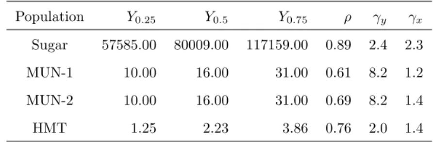
Table 1: Descriptive statistics of the variables of interest of the populations considered. ρis the population correlation coefficient betweeny andx, andγy andγx are respectively the population skewness coefficients ofy andx.
Population Y0.25 Y0.5 Y0.75 ρ γy γx Sugar 57585.00 80009.00 117159.00 0.89 2.4 2.3
MUN-1 10.00 16.00 31.00 0.61 8.2 1.2
MUN-2 10.00 16.00 31.00 0.69 8.2 1.4
HMT 1.25 2.23 3.86 0.76 2.0 1.4
number of seats in municipal council (population MUN-2). (iii) Finally, we considered the Hansen et al. (1983) population (population HMT), which is
N = 14000 units generated from a bivariate gamma population [see also Rao et al. (1990)]. A brief descriptive analysis of the various populations is given
in Table 1.
For each simulation, 1000 samples were selected to compute the empirical relative biasRB= 100%×(E[Ybα]−Yα)/Yαand the empirical relative root
mean square errorRRM SE = 100%×M SE[Ybα]1/2/Yα, where E[·] and
M SE[·] denote respectively the empirical expectation and mean square error. Simple random sampling and stratified random sampling are used to select the
samples. The population quartilesY0.25,Y0.5 andY0.75 are the parameters of
interest.
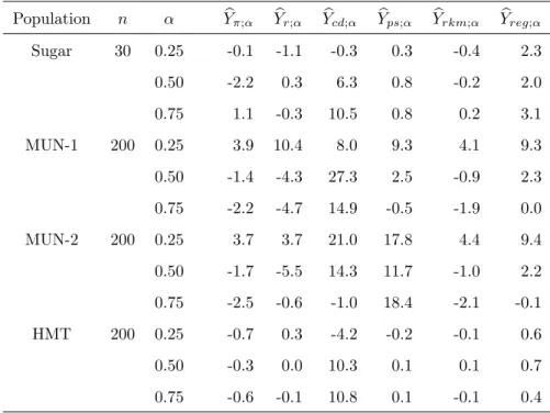
Table 2 reports the empirical relative bias (RB) under simple random sampling. The RBs of the proposed estimator is of a reasonable range compared with the RBs of the alternative estimators which can have a RB larger 10% in some cases. With the MUN-1 and MUN-2 populations, some estimators ofY0.25can have a large positive RB. Note that the proposed
Table 2: RB×100 of estimators of Yα, with α = 0.25, 0.5 and 0.75, under simple random sampling.
Population n α Ybπ;α Ybr;α Ybcd;α Ybps;α Ybrkm;α Ybreg;α Sugar 30 0.25 -0.1 -1.1 -0.3 0.3 -0.4 2.3 0.50 -2.2 0.3 6.3 0.8 -0.2 2.0 0.75 1.1 -0.3 10.5 0.8 0.2 3.1 MUN-1 200 0.25 3.9 10.4 8.0 9.3 4.1 9.3 0.50 -1.4 -4.3 27.3 2.5 -0.9 2.3 0.75 -2.2 -4.7 14.9 -0.5 -1.9 0.0 MUN-2 200 0.25 3.7 3.7 21.0 17.8 4.4 9.4 0.50 -1.7 -5.5 14.3 11.7 -1.0 2.2 0.75 -2.5 -0.6 -1.0 18.4 -2.1 -0.1 HMT 200 0.25 -0.7 0.3 -4.2 -0.2 -0.1 0.6 0.50 -0.3 0.0 10.3 0.1 0.1 0.7 0.75 -0.6 -0.1 10.8 0.1 -0.1 0.4 small.
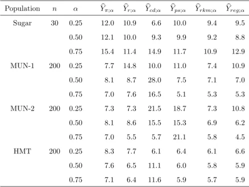
The efficiency of the estimators is measured by the empirical relative root mean square errors (RRMSE) which are reported in Table 3. We notice that the proposed estimator performs well in all situations. The proposed estimator is also more robust than its competitors. The proposed estimator for Yα is the
value of the inverse distribution function taken onαbreg instead ofα; where
b
αreg is defined in (16). As the distribution function is based upon the H´ajek type distribution function given by (3), we notice a clear improvement of using
b
αreg instead ofα, because the RRMSEs of the proposed estimator is usually smaller than of the the RRMSEs of the H´ajek estimatorYbπ;α, except with
Table 3: RRM SE×100 of estimators ofYα, withα= 0.25, 0.5 and 0.75, under simple random sampling.
Population n α Ybπ;α Ybr;α Ybcd;α Ybps;α Ybrkm;α Ybreg;α Sugar 30 0.25 12.0 10.9 6.6 10.0 9.4 9.5 0.50 12.1 10.0 9.3 9.9 9.2 8.8 0.75 15.4 11.4 14.9 11.7 10.9 12.9 MUN-1 200 0.25 7.7 14.8 10.0 11.0 7.4 10.9 0.50 8.1 8.7 28.0 7.5 7.1 7.0 0.75 7.0 7.6 16.5 5.1 5.3 5.3 MUN-2 200 0.25 7.3 7.3 21.5 18.7 7.3 10.8 0.50 8.1 8.6 15.5 15.3 6.9 6.2 0.75 7.0 5.5 5.7 21.1 5.8 4.5 HMT 200 0.25 8.3 7.7 6.1 6.4 6.1 6.6 0.50 7.6 6.5 11.1 6.0 5.8 5.9 0.75 7.1 6.4 11.6 5.9 5.7 5.9
can be more efficient than alternative estimators, especially when estimating
Y0.5andY0.75.
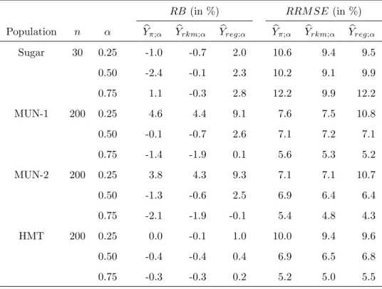
In Table 4, we have the RBs and the RRMSEs under stratified simple random sampling. We observe a small RB for all the estimators, except for estimators ofY0.25 of the MUN-1 and MUN-2 populations. With MUN-1 and MUN-2
populations, the RRMSEs of the proposed estimator is generally smaller than the RRMSE’s ofYbrkm(t). With the HMT population, the proposed estimator
andYbrkm(t) have similar RRMSEs.
Note that Ybrkm(t) is usually the most efficient estimator. The proposed estimator is slightly less accurate thanYbrkm(t), but much simpler to implement than Ybrkm(t). For medians, the proposed estimators is the most
Table 4: RB×100RRM SE×100 of estimators ofYα, withα= 0.25, 0.5 and 0.75, under stratified sampling with proportional allocation.
RB (in %) RRM SE (in %)
Population n α Ybπ;α Ybrkm;α Ybreg;α Ybπ;α Ybrkm;α Ybreg;α
Sugar 30 0.25 -1.0 -0.7 2.0 10.6 9.4 9.5 0.50 -2.4 -0.1 2.3 10.2 9.1 9.9 0.75 1.1 -0.3 2.8 12.2 9.9 12.2 MUN-1 200 0.25 4.6 4.4 9.1 7.6 7.5 10.8 0.50 -0.1 -0.7 2.6 7.1 7.2 7.1 0.75 -1.4 -1.9 0.1 5.6 5.3 5.2 MUN-2 200 0.25 3.8 4.3 9.3 7.1 7.1 10.7 0.50 -1.3 -0.6 2.5 6.9 6.4 6.4 0.75 -2.1 -1.9 -0.1 5.4 4.8 4.3 HMT 200 0.25 0.0 -0.1 1.0 10.0 9.4 9.6 0.50 -0.4 -0.4 0.4 6.9 6.5 6.8 0.75 -0.3 -0.3 0.2 5.2 5.0 5.5 accurate estimator.
We now propose to investigate the conditional relative biases of the proposed estimator by using the sample means of the auxiliary variable. For this purpose, the 1000 selected samples were ordered according to the mean of the
auxiliary variable. Then this ranking was used to create 20 groups of 50 observations each. Conditional relative biases are then obtained by calculating
the values ofRB for each of the 20 groups.
Figure 1 displays the conditional relative biases of the estimators of the first quartile under simple random sampling from the Sugar population. We observe that the H´ajek type estimator clearly exhibits the worst conditional
Figure 1: Conditional relative biases of estimates ofY0.25 under simple random
sampling from the Sugar-1 population withn= 30.
45 50 55 60 65 70 75 Group mean of x -10 -5 0 5 10 RB (in %) Proposed Rao el al. Hajek
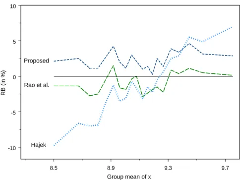
Figure 2: Conditional relative biases of estimates ofY0.5 under simple random
sampling from the MUN-1 population withn= 200.
8.5 8.9 9.3 9.7 Group mean of x -10 -5 0 5 10 RB (in %) Rao et al. Proposed Hajek
performance with a linear trend as the groupx-mean increases. The conditional RB of the proposed estimator and the Rao et al. (1990) estimator does not seem to be affected by variation in the group mean ofx. The Rao et al. (1990) estimator has a bias which is slightly smaller than the bias of the
proposed estimator.
Figure 2 displays the conditional relative biases of the estimators of the median under simple random sampling from the MUN-1 population. The conditional RB of the proposed estimator and the Rao et al. (1990) estimator
does not seem to be affected by variation in the x-mean.
7
Discussion
The proposed estimator is based on the regression estimator of the population mean, which is a technique widely used for survey data. The proposed estimator is a practical procedure that can be applied to many standard
surveys. As the proposed estimator is based upon first-order inclusion probabilities and the regression estimator, it can be easily implemented ith
multi-stage sampling designs.
Alternative estimators proposed by Chamber and Dunstan (1986) and Rao et al. (1990) can slightly be more accurate than the proposed estimator. However, in order to compute these alternative estimators, it is necessary to know the auxiliary variable for the entire population. The Rao et al. (1990) estimator also requires the joint inclusion probabilities, which are usually unknown with multi-stage designs. The proposed estimator is computationally
simpler because it is free of joint inclusion probabilities, it is based on the regression estimator and it can be computed when the auxiliary variable is not
known for the non-sampled units.
The accuracy of the proposed estimator can also be improved by inverting the Rao et al. (1990) estimator of the distribution function (or any other
estimators) rather than the H´ajek type estimator of distribution function. We have considered the regression estimator to account for the auxiliary
information. Other type of estimators based upon auxiliary information [Huang and Fuller (1978), Deville and S¨arndal (1992), Chen and Sitter (1999),
Breidt and Opsomer (2000), etc.] can also be used to improve the accuracy of the proposed estimator. The proposed estimator can be easily extended to these estimators. The proposed estimator can also be generalized to several auxiliary variables, since the regression estimator can be easily extended to
accommodate this situation.
A
Proof of Lemma 1
We have that Y∗α= 1 N X i∈U yα∗;i= 1 N X i∈U φ−1(F◦(yi)) +zκ, (20) F◦(yi) =Ri, (21) whereRi=N−1(rank(yi)−0.5) andrank(yi) is the rank of observationyiinthe population andφ−1(·) is the quantile function of aN(0,1) distribution.
By substituting (21) into (20), we have that
Y∗α= 1 N X i∈U φ−1(Ri) +zκ= 1 N(S<0.5+S>0.5+S0.5) +zκ (22) with S<0.5= X i∈U φ−1(Ri)δ(Ri <0.5), S>0.5= X i∈U φ−1(Ri)δ(R i >0.5), S0.5= X i∈U φ−1(Ri)δ(Ri= 0.5).
It is clear thatS0.5= 0. Consider a unit isuch thatrank(yi)<(N+ 1)/2.
This implies that Ri<0.5. Thus
S<0.5= X r<(N+1)/2 φ−1((r−0.5)/N), (23) S>0.5= X r<(N+1)/2 φ−1((N−r+ 1−0.5)/N) = = X r<(N+1)/2 φ−1(1−(r−0.5)/N). (24) Substituting (23) and (24) into (22), we obtain
Y∗α= 1 N X r<(N+1)/2 φ−1((r−0.5)/N) +φ−1(1−(r−0.5)/N) +zκ. (25) As the normal distribution is symmetric, we have thatφ−1(p) =−φ−1(1−p).
Hence the sum in (25) equal zero. This implies that
Y∗α=zκ. (26) AsF◦(Yα) =N−1(rank(Yα)−0.5),rank(Yα) =dαNe, and
κ=N−1(dαNe −0.5) , we have that
F◦(Yα) =κ (27) We also have that
F◦(Yα) =φ(φ−1(F◦(Yα))) =φ(Ψ(Yα)). (28) Equations (27) and (28) implies that
φ(Ψ(Yα)) =κ. (29)
As zκ is theκ-th quantile of a normalN(0,1) distribution, we have that
φ(zκ) =κwhich combined with (29) gives
Thus, the last expression implies
zκ= Ψ(Yα), (30) as φ(·) is a bijective function. Combining (26) with (30), we have that
Ψ(Yα) =Y∗α. The Lemma follows.
B
Proof of Theorem 1
Asφ(·) is twice differentiable, a first order Taylor expansion implies that
φ(y∗reg;α)−φ(Y ∗ α) = (y∗reg;α−Y ∗ α)f(Y ∗ α) +Op(|y∗reg;α−Y ∗ α|2), (31) wheref(y) is the density of aN(0,1) distribution. Equation (26) implies that
φ(Y∗α) =φ(zκ) =κ. Thus, asκ→αasN → ∞, limN→∞φ(Y ∗ α) =αand we have that φ(y∗reg;α)−α= (y∗reg;α−Y ∗ α)f(Y ∗ α) +Op(n−1), (32) becausey∗reg;α−Y ∗ α=Op(n−1/2).
AsQ(α) is twice differentiable, a first order Taylor expansion implies that
Q(φ(y∗reg;α))−Q(α) = (φ(y∗reg;α)−α)Q0(α) +Op(|φ(y∗reg;α)−α|2) whereQ0(α) =∂Q(α)/∂α. Assumption (18) and (32) imply that
Q(φ(y∗ reg;α))−Q(α) = (y∗reg;α−Y ∗ α)f(Y ∗ α)Q0(α) +Op(n−1), (33) asf(Y∗α) is bounded. Using assumption (19), equation (33) implies that
b F◦−1(φ(y∗reg;α))−Fb◦−1(α) = (y∗reg;α−Y ∗ α)f(Y ∗ α)Q0(α) +Op(n−1). (34) AsFb◦−1(φ(y∗
reg;α)) =Ybreg;αandFb◦−1(α) =Ybα, equation (34) becomes
b Yreg;α=Ybα+ (y∗reg;α−Y ∗ α)f(Y ∗ α)Q0(α) +Op(n−1).
which implies b Yreg;α−Yα=Ybα−Yα+ (y∗reg;α−Y ∗ α)f(Y ∗ α)Q0(α) +Op(n−1). Thus, the last expression combined with assumption (17) and (18) imply
|Ybreg;α−Yα|=Op(n−1/2).
References
[1] Bahadur, R. R. (1966). A note on quantiles in large samples. The Annal of Mathematical Statistics, 37, 577-580.
[2] Berger, Y. G. and Skinner, C. J. (2003). Variance estimation of a low-income proportion. Journal of the Royal Statistical Society Series C, 52, 457-468.
[3] Berger, Y. G. and Skinner, C. J. (2005). A Jackknife Variance Estimator for Unequal Probability Sampling.Journal of the Royal Statistical Society Series B, 67, 79-89.
[4] Berger, Y. G. (2007). A jackknife variance estimator for unistage stratified samples with unequal probabilities. Biometrika, 94, 953-964.
[5] Berger, Y. G. and De La Riva Torres, O. (2012). A unified theory of empir-ical likelihood ratio confidence intervals for survey data with unequal prob-abilities. Proceedings of the Survey Research Method Section of the Amer-ican Statistical Association, Joint Statistical Meeting, San Diego, 15pp. [6] Breidt, F. J. and Opsomer, J. D. (2000). Local polynomial regression
es-timators in survey sampling. The Annal of Mathematical Statistics, 28, 1026-1053.
[7] Cannamela, C., Garnier, J. and Iooss, B. (2008). Controlled stratification for quantile estimation. Annals of Applied Statistics, 4, 1554-1580.
[8] Cassel, C. M., S¨arndal, C. E. and Wretman, J. H. (1976). Some results on generalized difference estimation and generalized regression estimation for finite populations. Biometrika, 63, 615-620.
[9] Cassel, C. M., S¨arndal, C. E. and Wretman, J. H. (1977). Foundation of inference in survey sampling. John Wiley, New York.
[10] Chambers, R. L. and Dunstan, R. (1986). Estimating distribution functions from survey data. Biometrika, 73, 597-604.
[11] Chen, J. and Sitter, R. R. (1999). A pseudo empirical likelihood approach to the effective use of auxiliary information in complex surveys. Statistica Sinica, 9, 385-406.
[12] Deville, J. C. and S¨arndal, C. E. (1992). Calibration estimators in survey sampling. Journal of the American Statistical Association, 87, 376-382. [13] EUROSTAT (2003). ”Laeken” Indicators-Detailed
Cal-culation Methodology, Directorate E: Social Statis-tics, Unit E-2: Living Conditions, DOC.E2/IPSE/2003. http://www.cso.ie/en/media/csoie/eusilc/documents/Laeken%20Indicators%20-%20calculation%20algorithm.pdf.
[14] Francisco, C. A. and Fuller, W. A. (1991). Quantile estimation with a complex survey design. Annals of Statistics, 19, 454-469.
[15] Hansen, M. H., Madow, W. G. and Tepping, B. J. (1983). An evaluation of model-dependent and probability-sampling inferences in sample surveys. Journal of the American Statistical Association, 78, 776-793.
[16] Huang, E. T. and Fuller, W. A. (1978). Nonnegative regression estimation for survey data. In Proc. American Statistical Association (Social Statistics Section), 300-303.
[17] Isaki, C. T. and Fuller, W. A. (1982). Survey design under the regression super-population model. Journal of the American Statistical Association, 77, 89-96.
[18] Law, A. M. and Kelton, W. D. (1991). Simulation Modeling and Analysis, 2nd Ed. McGraw-Hil, New York.
[19] Lehmann, E. L. (1999). Elements of large-sample theory, New York: Springer-Verlag.
[20] Nyg˚ard, F. and Sandstr¨om, A. (1985). The estimation of the Gini and the entropy inequality parameters in finite populations. Journal of Official Statistics, 4, 399-412.
[21] Osier, G. (2009). Variance estimation for complex indicators of poverty and inequality using linearization techniques. Journal of the european Survey Research Association, 3, 167-195.
[22] Rao, J. N. K., Kovar, J. G. and Mantel, H. J. (1990). On estimating distri-bution functions and quantiles from survey data using auxiliary informa-tion. Biometrika, 77, 365-375.
[23] Rao, J. N. K., Wu, C. F. J. and Yue, K. (1992). Some recent work on resampling methods for complex surveys. Survey Methodology, 18, 209-217.
[24] Robinson, P. M. and S¨arndal, C. E. (1983). Asymptotic properties of the generalized regression estimator in probability sampling. Sankhya B, 45, 240-248.
[25] S¨arndal, C. E., Swensson, B. and Wretman, J. H. (1992). Model Assisted Survey Sampling, New York, Springer Verlag.
[26] Serfling, N. (1980). Approximation Theorems of Mathematical Statistics, New York: Wiley.
[27] Silva, P. L. D. and Skinner, C. J. (1995). Estimating distribution func-tions with auxiliary information using poststratification. Journal of Official Statistics, 11, 277-294.
[28] Verma, V. and Betti, G. (2011). Taylor Linearization Sampling Errors and Design Effects for Poverty Measures and Other Complex Statistics. Journal of Applied Statistics, 38, 1549-1576.
[29] Woodruff, R. S. (1952). Confidence intervals for medians and other position measures. Journal of the American Statistical Association, 47, 635-646. [30] Wu, C. and Rao, J. N. K. (2006). Pseudo-empirical likelihood ratio
con-fidence intervals for complex surveys. Canadian Journal of Statistics, 34, 359-375.