Price Prediction of Selected Cryptocurrencies Using Machine Learning Algorithms

Czech Technical University in Prague

Faculty of Mechanical Engineering

Department of Instrumentation and Control Engineering

Bachelor’s Thesis

Price Prediction of Selected

Cryptocurrencies Using Machine

Learning Algorithms

Author:

František Grossmann

Supervisor:

Ing. Matouš Cejnek

BACHELOR‘S THESIS ASSIGNMENT

424937

Personal ID number:

Grossmann Frantisek

Student's name:

Faculty of Mechanical Engineering

Faculty / Institute:

Department / Institute: Department of Instrumentation and Control Engineering Bachelor of Mechanical Engineering

Study program:

Information and Automation Technology

Branch of study:

II. Bachelor’s thesis details Bachelor’s thesis title in English:

3ULFH3UHGLFWLRQRI6HOHFWHG&U\SWRFXUUHQFLHV8VLQJ0DFKLQH/HDUQLQJ$OJRULWKPV

Bachelor’s thesis title in Czech:

3redikcHvývoje cenyY\EUDQêFKkryptoměnSRPRFtVWURMRYpKRXþHQt

Guidelines:

- introduce deep learning and recurrent netw. used as a tool for predicting the development of a cryptocurrency's price. - select appropriate prediction models and apply technical indicators as features to predict a cryptocurrency's price. - compare strategies used in traditional prediction methods with methods used in Machine Learning and it's results.

Bibliography / sources:

Shai Shalev-Shwartz, Shai Ben-David: "Understanding Machine Learning: From Theory to Algorithms", Cambridge University Press, 2014.

John V. Guttag : "Introduction to Computation and Programming Using Python" Massachusetts Institute of Technology, 2013

Arvind Narayanan, Joseph Bonneau, Edward Felten, Andrew Miller, Steven Goldfeder: "Bitcoin and Cryptocurrency , Princeton University, 2016

Name and workplace of bachelor’s thesis supervisor:

Ing. Matouš Cejnek, U12110.3

Name and workplace of second bachelor’s thesis supervisor or consultant:

Deadline for bachelor thesis submission:..201

Date of bachelor’s thesis assignment: ..2018

Assignment valid until: _____________

___________________________ ___________________________

___________________________

prof. Ing. Michael Valášek, DrSc.

Dean’s signature Head of department’s signature

Ing. Matouš Cejnek

Supervisor’s signature

Prohlášení

Prohlašuji, že jsem tuto bakalářskou práci vypracoval samostatně s tím, že její výsledky mohou být dále použity podle uvážení vedoucího bakalářské práce jako jejího spoluautora. Souhlasím také s případnou publikací výsledků bakalářské práce nebo její podstatné části, pokud budu uveden jako její spoluautor. Dále prohlašuji, že všechny použité prameny jsou citovány.

V Praze dne ... ... František Grossmann

Acknowledgment

Abstract

The aim of this bachelor’s thesis is to investigate the efficiency and application of machine learning algorithms to predict the future price of a cryptocurrency. The first half of the paper deals with a brief description of cryptocurrencies and the technology backing the whole ecosystem. Following an evaluation of traditional methodologies used to forecast financial times series and how the cryptocurrency market reacts to the application of these methods. Appropriate features are en-gineered from data-sets of selected cryptocurrencies and applied to the machine learning algorithms. These algorithms are eventually tested. Their performances are reviewed and a conclusion is drawn from the results.

Keywords

Cryptocurrencies, Machine Learning, Artificial Neural Networks, Recurrent Neural Networks, Data Analysis, Technical Indicators.

Abstrakt

Řadu let je oblastí velkého zájmů jak akademiků, tak ekonomů predikce fi-nančních časových řad. Potenciál správně predikovat aktiva libovolného druhu se dramaticky zlepšil s nástupem umělé inteligence.

Specificky, aplikace strojového učení na časové řady je tématem mnoha diskuzí. Ačkoliv bylo vydáno několik vědeckých prací a článků na zmíněné téma, pouze hrstka se zabývá užitím umělé inteligance v predikci cen jednotlivých kryptoměn. Tato bakalářská práce se zabývá aplikací algoritmů strojového učení na klíčové technické indikátory a jejích účinností v predikci vybrané kryptoměny. Modely a indikátory jsou naprogrogramované v Pythonu. V závěru této práce se porov-nají výsledky predikačních modelů a srovporov-nají s doposud zveřejněnými výsledky v tomto oboru.

Klíčová slova

Kryptoměny, Strojové učení, Neuronové sítě, Rekurentní sítě, datová analytika, Technické indikátory.

Contents

1 Introduction 1

1.1 Outline of the thesis . . . 2

2 Related research 3 2.1 Efficient Market Hypothesis . . . 3

2.2 Literature review . . . 4

3 Cryptocurrencies 7 3.1 Overview . . . 7

3.1.1 The Cryptocurrency Market . . . 8

4 Machine Learning 10 4.1 Fundamental Algorithms . . . 10

4.2 Introduction to Neural Networks . . . 12

4.2.1 Feed-Forward Neural Networks . . . 12

4.2.2 Neuron . . . 13

4.2.3 Network Structure . . . 14

6 Practical Implementation 26 6.1 Technical Background . . . 26 6.2 Data Analysis . . . 27 6.2.1 Data Fundamentals . . . 27 6.2.2 Data Processing . . . 29 6.3 Methodology . . . 33 6.3.1 Motivation . . . 33

6.3.2 Technical Indicators as Features . . . 33

6.3.3 Sliding Window . . . 35

6.4 Prediction Model Evaluation . . . 36

6.4.1 Recurrent Network - LSTM . . . 36

6.4.2 Results . . . 38

7 Conclusion 42

List of Figures

3.1 The market capitalization reached it’s peak in January 2018 with a value surpassing 800 billion dollars. Source [20]. . . 8 3.2 Chart depicting Bitcoin price volatility against the USD. Source [22] 9 4.1 A simple illustration of how the learning phase works in supervised,

unsupervised and reinforcement learning. . . 11 4.2 An image of a biological neuron [25]. . . 12 4.3 An illustrative example of a computational neuron. . . 13 4.4 A scheme of the multi-layer perceptron with one hidden layer. This

illustration does not reflect the applied MLP for the task of this thesis. . . 15 4.5 A simple example of the gradient descent convergence towards the

global minimum of the cost function, including a depiction of the hyperparameter η and their possible settings . . . 17 4.6 Flowchart illustrating how the backpropagation technique works.

The blue arrows defining the forward flow of information and the red one’s backward flow. For simplicity sake, the biases were omit-ted. . . 19 5.1 The straightforward diagram presents a recurrent cell. It takes in

an input xt and outputs a valueht of the hidden layer in time t. . 22 5.2 Unrolling of RNN dynamics. . . 22

List of Figures

5.3 A scheme of a Long Short-Term Memory cell unit. The cell is structured into four gates. The Input Gate evaluates what values need to be updated. The Forget Gate calculates whether to keep the incoming information or not. The CEC Cell is responsible for preventing vanishing gradients. The Output Gate decides on the output [36]. . . 23 6.1 In our thesis, we work with Market Data as seen in the table - The

Four Essential Types of Financial Data [46]. . . 28 6.2 Graph showing normalized input feauture - close price.

Cryptocur-reny pair LTC/USD. . . 31 6.3 Graph indicating the ratio of 80% to 20% of training/testing data. 31 6.4 Depiction of the Simple Moving Average feature. The image clearly

shows how reactive the individually set MA are to price changes. This graph depicts the first 600 minutes of trading. . . 34 6.5 Denormalized close price data against the prediction of the

cur-rency pair LTC/USD. . . 38 6.6 A detailed look on the denormalized close price against the

pre-diction of the currency pair LTC/USD. The graph is a 120 minute time frame in 15 minute time-steps. . . 39 6.7 This figure shows the training and validation loss of our

RNN-LSTM model. The decay of the optimizer Adam is set to 0.25. 12 epochs were used for training the model and the test validation value did not decrease in a continuous manner. This is a sign that we are overfitting the data. . . 39 8.1 Denormalized close price data against the prediction of the

cur-rency pair BTC/USD. . . 47 8.2 A detailed look on the denormalized close price against the

pre-diction of the currency pair BTC/USD. The graph is a 120 minute time frame in 15 minute time-steps. . . 48 8.3 This figure shows the training and validation loss of our

RNN-LSTM model. The decay of the optimizer Adam is set to 0.25. 12 epochs were used for training the model and the test validation value did not decrease in a continuous manner. This is a sign that we are overfitting the data. . . 48 8.4 Denormalized close price data against the prediction of the

cur-rency pair ETH/USD. . . 49 9

List of Figures

8.5 A detailed look on the denormalized close price against the pre-diction of the currency pair ETH/USD. The graph is a 120 minute time frame in 15 minute time-steps. . . 49 8.6 This figure shows the training and validation loss of our

RNN-LSTM model. The decay of the optimizer Adam is set to 0.25. 12 epochs were used for training the model and the test validation value did not decrease in a continuous manner. This is a sign that we are overfitting the data. . . 50 8.7 Denormalized close price data against the prediction of the

cur-rency pair ETH/USD. . . 50 8.8 A detailed look on the denormalized close price against the

pre-diction of the currency pair ETH/USD. The graph is a 120 minute time frame in 15 minute time-steps. . . 51 8.9 This figure shows the training and validation loss of our

RNN-LSTM model. The decay of the optimizer Adam is set to 0.25. 12 epochs were used for training the model and the test validation value did not decrease in a continuous manner. This is a sign that we are overfitting the data. . . 51

List of Tables

6.1 Table with historical price data. This example shows the LTC-USD dataset . . . 30 6.2 Parameters settings of the RNN-LSTM model that yield the best

results. . . 37 6.3 The table exhibits the numerical results of the prediction model.

We present four metrics, MAE, MSE, Train Loss and Test Loss. . 40

1

|

Introduction

The prediction of financial time series has been an area of great interest through-out fields such as computer science, economics, and statistics. An accurate model can yield significant profits which makes it a key driver for research. Over the years a wide range of instruments and approaches were developed both by aca-demics and industry professionals. In traditional markets, the methods used to evaluate the asset’s future price fall into three main categories: fundamental anal-ysis, technical analysis and technological methods [1].

Fundamental analysis involves the study of a company’s fundamentals, such as it’s financial situation, market position, company management and other qualita-tive and quantitaqualita-tive factors. The analysis should determine whether the market has incorrectly priced an asset [2]. Technical analysis, on the other hand, is an analysis methodology based solely on the study of past market data, price and volume [3].

Investors forecasting an asset’s price believe that all the fundamental informa-tion is already projected into the historical price. Particular visual formainforma-tions in charts, alongside with techniques such as the Simple Moving Average provide the basis to predict a future price.

Breakthroughs in technology, particularly in artificial intelligence (AI) lead to wide adoption of these new technologies in the financial market. Specifically, Machine learning a sub-field of AI gained wide recognition among individuals and financial institutions. Technical analysis alone gained a totally new dimension and from a naturally qualitative tool turned into a quantitative tool.

Chapter 1. Introduction

1.1

Outline of the thesis

The following points provide an outline of this thesis:

• Chapter 2In this chapter we introduce the Efficient Market Hypothesis as

a cornerstone theory in the field of financial market predictions. Following a literature review of research involving machine learning applied to price prediction of securities

• Chapter 3We uncover the topic of cryptocurrencies and outline their

tech-nical background and dive into the dynamic of the cryptocurrency market. • Chapter 4 This chapter examines the most well-known machine learning

algorithms, Neural Networks and detailing their working and mathematical formulation.

• Chapter 5 Following an introduction into Deep Learning with Recurrent

Neural Networks.

• Chapter 6 This chapter describes the practical aspect of this thesis, how

we collected and processed our data, what methodology can enhance the prediction model and our price prediction strategy.

• Chapter 7In this chapter we evaluate the achieved results by our

predic-tion model.

• Chapter 8 This chapter concludes our findings and examines the results

from a general perspective.

2

|

Related research

This chapter begins with the introduction of Efficient Market Hypothesis a critical theory in forecasting security prices in the finance market. Later on, we will review research that has been conducted so far in the area of cryptocurrency price prediction.

2.1

Efficient Market Hypothesis

“The price of a security at any time fully reflects all available information; hence, it is impossible for investors to make a profit above the average market returns.” — Eugene Fama

The last century saw an immense concentration of research and mathematical complexity pour into the finance market. One assumption of financial economics that gained significant recognition among professionals over the years is the Ef-ficient Market Hypothesis (EMH). The theory claims that market prices fully reflect all available information; hence a market with fully reflected information is called efficient [4]. Authors of the theory Paul A. Samuelson and Eugene F. Fama declared that securities always trade at their fair value, making it impossi-ble for traders to outperform the market with expert tools or market timing. New information is quickly integrated into the market price. The investor is essentially forced to purchase riskier investments [5]. In 1970 Fama formalized a notation of the non-predictability of market prices by:

Chapter 2. Related research

The Reality of Efficient Market Hypothesis

Despite the theoretically solid nature of EMH, the application and research over the past 30 years has proved several times that certain market phenom-ena contradict with assumptions of EHM. For example, stock markets exhibit seasonal trends which can be exploited with trading strategies allowing for high winter returns and low summer returns [6]. Another major alternative to the EHM is behavioral psychology in finance. Behavioral finance believes that the market reflects all of the imperfections and ineffective decisions made by humans, reflect-ing their desires, goals, motivations, and overconfidence. These biases also lead to tendencies to underestimate new information and have a generally one-sided view of the market [7].

Although intellectuals from academia point to evidence in support of the EHM theory, many well-known individuals in the financial sector advocate strongly against it. Most notably Warren Buffet who outperformed the market by detecting mispriced securities to achieve significant profits [8].

2.2

Literature review

The practical use of machine learning in finance has been studied for several decades. Research conducted on the efficiency of machine learning methods to predict a cryptocurrency’s price is limited.

Jang and Lee implemented Bayesian neural networks along with features de-rived from the fundamentals of Bitcoin and blockchain technology. The authors confirmed high volatility of Bitcoin and designed a well-performing price time series predicator [9]. Another study issued by Madan, Saluja and Zhao investi-gated the problem of predicting Bitcoin’s price fluctuations from a classification perspective. An accuracy of 98.7% was achieved for daily predictions and 50-55% using 10 minute time intervals [10]. Another paper examined the correlation be-tween fundamental economic variables, sentimental analysis, and Bitcoin price. Geourgoula et. al. applied support vector machines to their study and found that the frequency of Wikipedia views and the networks hash rate had a positive cor-relation with Bitcoins price. Owing to vast amounts of available data, sentiment is increasingly utilized as a predictor of cryptocurrency price. Zhang and Shah describe the use of nonparametric classification for predicting trends. They intro-duce a latent source model1_{, discussed by Chen, Nikolov and Shah [12]. Namely,}

Bayesian regression is used for predicting Bitcoin price movements, resulting in a nearly double gain of their initial investment in a 60 day period [13]. Alex Greaves and Benjamin Au engineered blockchain-network features to analyze the network’s influence on Bitcoin price. By applying the features to SVM and ANN 1_{A latent source is designated from latent variables which present characteristics not directly} observable, but rather an approach which underlines a phenomenon of a system from a set of variables [11].

Chapter 2. Related research

algorithms, they achieved a price movement accuracy of 55% [14]. The results achieved by Alex Greaves and Benjamin Au can be considered as optimistic and in a sense contradict the EHM theory. Several studies have taken into account sentiment analysis which plays an increasingly important role in today’s society highly influenced by social media. Young Bin Kim et al. studied online cryp-tocurrency communities in order to predict price fluctuations using a well-known solution for predicting currency and share value called the Granger casuality test [15]. The authors of the study came to a conclusion that comments and opinions on social media regarding cryptocurrencies do affect the price. Several articles and studies began to recently experiment with the application of Recurrent neu-ral networks (RNN) on Bitcoin data. Evidence suggests that RNNs can provide improved performance. In his paper [16] Sean McNally aimed to predict the di-rection of Bitcoin price against the USD. Both RNN and LSTM (Long short term memory) networks were tested on daily prices of Bitcoin. The LSTM net-work reached the best results on a 100-day window with an accuracy of 52%. Douglas Garcia Torres and Hongliang Qiu analyzed the performance of ARIMA (AutoRegressive Integrated Moving Average) and RNNs on sample Bitcoin data. They proved that RNN provides better performance over non-dynamic ARIMA. From the prediction accuracy point of view, the choice between LSTM and GRU (Gated Recurrent Unit) do not play a major role [17].

3

|

Cryptocurrencies

This chapter introduces a new digital form of currency known as a cryptocurrency. The asset is discussed in regard to the market that it is situated in.

3.1

Overview

A cryptocurrency is a digital asset designed to work as a medium of exchange using cryptography to secure it’s transactions, prevent tampering with payments and to encode the rules for creating new units of currency. As opposed to tra-ditional finance systems, cryptocurrencies operate on a decentralized peer-to-peer network where each transaction is facilitated into a public ledger called the blockchain. This enables participants in the network to send assets directly, with-out any intermediary. Cryptocurrencies are transferred between parties through the use of a public and private key.

Bitcoin, created in 2009 is currently the most well-known cryptocurrency as well as the first decentralized currency to work on a blockchain. Bitcoin is an en-tirely virtual currency, no physical coins exist. New bitcoins are created through a process called mining, which is a technique to validate transactions by the use of computational power. Miners provide processing power to solve complex math-ematical/cryptographic puzzles and receive bitcoins for successfully validating a transaction. The solution to this problem is called Proof-of-Work and acts as a signature that the miner expended significant computing power. A new block is mined every 10 minutes and is added to the blockchain. The Proof-of-Work algorithm forces the creation of new blocks to be placed in chronological order, making it exceptionally difficult to reverse previously approved transactions. The mining process furthermore disables double-spending, an issue burdening current financial institutions. The aforementioned properties of mining furthermore serve as a genuine security mechanism against fraudulent transactions [18],[19].

Chapter 3. Cryptocurrencies

3.1.1

The Cryptocurrency Market

The past few years have seen a significant breakthrough of cryptocurrencies in the world of finance. Since the launch of Bitcoin, more than 2,000 new cryptocurren-cies have been introduced with a majority of them functioning on the underlying blockchain technology. As of December 2018, the market capitalization of actively traded cryptocurrencies has surpassed 140 billion USD.

Figure 3.1: The market capitalization reached it’s peak in January 2018 with a value surpassing 800 billion dollars. Source [20].

Each cryptocurrency has a predetermined supply of coins/tokens1, essentially

setting a monetary policy against inflation. Therefore giving opportunity to a potentially dramatic increase in value. From the perspective of economic the-ory(cislo), whether a cryptocurrency represents a store of value or a medium ex-change is not clearly defined. Broadly speaking, cryptocurrencies presently serve as a medium of exchange and an asset for speculation. As a result of this, the market can be described as unique in contrast to other markets. Notable media coverage and an influx of wealth into the technology prompt a number of finan-cial institutions into exploring the adoption of cryptocurrencies and blockchain technologies.

1_{Tokens are a tradable asset or utility working on blockchain technology [21].} 8

Chapter 3. Cryptocurrencies

According to conducted research, the market is currently in a very volatile state (knížka bank of england). Some of the major factors influencing the volatility of the ecosystem are:

• Negative media coverage

• Unevenly distributed coin volume • Automated trading bots

• Insufficient institutional capital • Inadequate regulatory oversight • Security flaws

Figure 3.2: Chart depicting Bitcoin price volatility against the USD. Source [22] The novelty and instability of the market present an interesting opportunity to apply modern analytical techniques to forecast future prices of cryptocurrencies. Available API solutions for market data and an open source environment serve as a basis for creating useful libraries and tools for time series forecasts. We shall use these options to our advantage and feel it necessary to leverage machine learning algorithms to predict future prices of cryptocurrencies.

4

|

Machine Learning

The aim of this chapter is to introduce machine learning algorithms used to predict the future price a cryptocurrency. The general concept of each algorithm and its main uses are described. For optimization, we cover the hyperparameters via cross-validation.

4.1

Fundamental Algorithms

Machine learning is the ability of an algorithm to detect and extrapolate patterns from a given data set without being explicitly programmed. The algorithms adap-tively improve their performance as the number of samples available for learning increases. Machine learning tasks are divided by their feedback into two broad categories:

Supervised Learning

In supervised learning, an algorithm is presented with a data set containing instances which are associated with a label. Specifically, the learning process involves observing examples of a random vector x and a value y, and generating a function to predict y fromx by estimating a probability distributionp(y|x,D)

[23]. If the target output y is of a finite set of values (green, blue, red) then the learning problem is calledclassification. On the other hand when the target output yis a numerical, continuous value (price) then aregressionmodel is implemented. This type of prediction is suitable for algorithmic trading and will be applied in this thesis.

Unsupervised Learning

An unsupervised learning algorithm has presented a data set containing in-stances without a label. Similarly, the learning algorithm iterates through several examples of a random vectorx and attempts to learn the probability distribution

p(x) or discover hidden patterns without any explicit feedback. The most

com-mon task of unsupervised learning algorithms consists of dividing a dataset into clusters from respective inputs. An example of the most popular algorithm used in unsupervised learning is k-means.

Chapter 4. Machine Learning

Reinforcement Learning

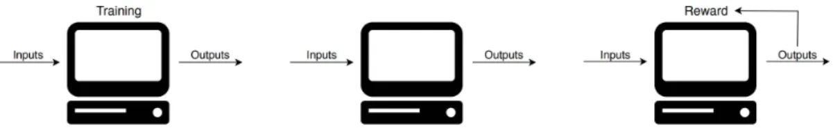
Reinforcement Learning (RL) is an area of machine learning, where an agent learns in an interactive environment by trial and error using feedback from its own actions and experiences in order to maximize a numerical signal reward. RL is considered one of three major machine learning paradigms along with supervised and unsupervised learning. The learning approach does not make use of a training dataset to learn patterns, instead, the agent must discover which actions yield the greatest reward. This process essentially works in a closed loop so the learning system’s actions influence its later inputs. In conclusion, Reinforcement Learning is characterized by three significant features: Closed-loop architecture, no direct instructions as to what actions to take, and where the consequences of actions along with rewards play out over a time period [24].

Reinforcement learning is gaining popularity in recent years and is widely applied in several devices and problems. For example, a mobile robot may decide whether to continue cleaning a room or returns to the battery charging station. It makes a decision based on the charge level of its battery and how quickly it manages to find the station in the past.

Figure 4.1: A simple illustration of how the learning phase works in supervised, unsupervised and reinforcement learning.

This section brought a brief overview of the three main areas of machine learn-ing. As the topic of this paper is to create a model, capable of performing a predic-tion on a provided data set with labeled instances, thus the outlined algorithms will be used for a supervised learning regression problem.

Chapter 4. Machine Learning

4.2

Introduction to Neural Networks

Neural Networks or Artificial Neural Networks (ANN) are computational models originally motivated by neural networks in biological brains. The fundamental functional units of the brain are called neurons and carry out highly complex computing tasks. Together with other neurons located in the brain, they form a large communication network with significant computing capacity. Each neuron consists of dendrites a cell body, axon and axon terminals. The cell body receives input signals from multiple dendrites and effectively processes them in the nucleus from where a definite output value is sent, through the axon, to its terminals.

Figure 4.2: An image of a biological neuron [25].

Formally, ANN are simplified technical constructs representing a collection of nonlinear statistical models that yield convincing results associated with learning tasks. Areas, where ANN have proven to be highly effective include computer vision, speech recognition, machine translation, time series forecasting and many more. Three major learning paradigms are used to address problems: supervised learning, unsupervised learning and reinforcement learning; with considerable use in regression and classification. Several models and learning methods have been developed over the years. The most commonly used are feed-forward neural net-works, convulational neural networks and recurrent neural networks to name a few.

Due to the predictive power and sustainable results obtained by research, the feed-forward neural network architecture presents a possible model suited for this task. In the following sections, we shall introduce the architecture, functioning, and training of ANN. The mathematics in this chapter stem profoundly from [26].

4.2.1

Feed-Forward Neural Networks

The feed-forward neural networks are the simplest neural network architecture devised. It is defined as a directed acyclic graph of nodes corresponding to neurons

Chapter 4. Machine Learning

and edges corresponding to links1_{. The nodes are arranged in n layers}

intercon-nected by edges that pass on the information. The output of a neuron in the i-th layer is connected to the input of a neuron in i+1 layer until reaching the output layer. So in a sense, this architecture has no feedback connections or form any cycles.

4.2.2

Neuron

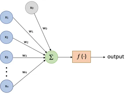
The functional building block of each ANN is a Neuron. Every neuron receives an input signal from which it derives an output. The first layer, marked blue, is called the input layer and represents vector features {(x1,x2, ...,xn)}. This layer is connected to the neuron via a link carrying a numeric weight{(w1,w2, ...,wj)}, determining the importance of respective inputs to the output [27]. The structure also incorporates a bias unit b, with a fixed value of 1 and our case associated with weightwj0.

Figure 4.3: An illustrative example of a computational neuron.

The neuron firstly computes the weighted sum of inputs to structure an acti-vation:

N

X _{(1) (1)}

Chapter 4. Machine Learning

zj =h(aj). (4.2) We defined (4.5) in order to bring more clarity into further equations. Super-script (1) and subSuper-script j inform the reader that the parameters are located in the first layer of the ANN. Furthermore (4.3) declares the activation outputs of neurons located in the hidden layer. To calculate the neurons activation’s of the output layer we proceed to the following formula

ak = M X i=1 w_kj(2)zj +w (2) k0 (4.3)

wherek=1,...,K corresponds to the number of outputs of the subsequent layer, in our case the second one. A generally accepted choice for the nonlinear activation functionh(·)is a sigmoid function, although more functions are gaining traction

in the field.

h ≡σ(a) = 1

1 +−_a (4.4)

From this stage, the outputs of neurons are transformed by an arbitrary acti-vation function to produce a final output of the entire network

yk(x,w) =σ M X j=1 w_kj(2)h N X i=1 w_ji(1)xi +w (1) j0 ! +w_k(2)₀ ! (4.5) This mathematical statement essentially states how forward propagation works. The model takes in a set of inputxi variables to propagate a set of output variables

yk restrained by the adjustable weight vectorw.

4.2.3

Network Structure

The most trivial neural network is a Single-Layer Network known as a Percep-tron. The model embodies N amount of weighed inputs that are directly fed into the output. The perceptron is considered to be the first machine learning algo-rithm. It’s was constructed by a US military institute for image recognition and laid down the fundamentals for other ANN to follow. Although seeming promis-ing, the perceptron was only capable of learning linearly separable patterns and could not withstand more complex problems. Eventually, theMulti-Layer Percep-tron (MLP) was introduced, adding more processing power and vastly increasing applicability to nonlinear problems.

Chapter 4. Machine Learning

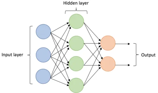
Figure 4.4: A scheme of the multi-layer perceptron with one hidden layer. This illustration does not reflect the applied MLP for the task of this thesis.

The MLP network consists of at least three layers - input layer, hidden layer, and an output layer. Apart from the input layer, each following layer comprises of N neurons, processing weighed inputs from the previous layer, gradually carrying the value to the successive layer. The hidden layers form the main computing body of neural networks and present one of the parameters of the network. The number of neurons and hidden layers have to be carefully considered when constructing the neural network. Applying too few neurons or hidden layers can result in an effect called underfitting. On the contrary, too many neurons or hidden layers in the structure lead to overfitting2. Figure 4.4 provides an illustration of the

multi-layer perceptron.

4.2.4

Learning

So far we have introduced neural networks as a class of nonlinear functions with predictive potential. As in the biological realm, the artificial neuron has to be trained in order to reach or recognize the desired pattern. This phase is critical and requires a careful adjustment of the parameters3 via a series of training steps

and methodologies.

Given our training set {(x1,y1), ...,(xn,yn)}, where xi is the input vector and yi the output vector for all i ∈ h1,ni. Neural network training is generally

Chapter 4. Machine Learning

of each individual training session. Although rigorous, the loss function provides information associated with a single training example. In order to support this observation, a cost or also known as cost function needs to be defined. It measures how well the overall training set is doing with respect to the input vector. The error function4 weighs the average of the previously mentioned loss function to

form the following:

E(w) = 1 2 N X n=1 ||y(xn,w)−tn||2 (4.6) Gradient Descent

The aim of training the neural network is to minimize the error function which we will achieve by using an optimization algorithm calledGradient Descent. The algorithm is a vector consisting of partial derivatives of the error function (4.6). Updates to the weights are expressed as:

w(τ+1)= (w)(τ)−η∆E(w(τ)) (4.7)

and indicate that the vector moves in the direction of the greatest decrease in the error function.τ designates to individual iteration steps and η >0 is known

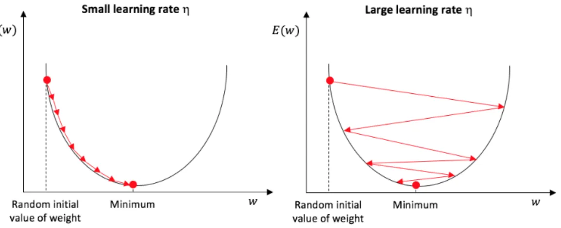
as the step size or learning rate. It represents a hyper-parameter that needs to be adjusted manually and plays the most significant role in the learning process. It determines how quickly the neural network adjusts to correct outputs in the training set, or in other words how quickly do the parameters update and when will the gradient decent find the optimum of the cost function. If the value of the hyper-parameter is set too low the gradient will take too long to calculate the minimum. On the other hand, a large learning rate can lead to divergence of the error function. A rule of thumb is to set the learning rate in an interval of

h0.01−0.001i

Although we have a fundamental description of how to update parameters of the network, the heart of how a neural network actually learns lies in an iterative approach calledBackpropagation. The backpropagation method gives an efficient

way to compute partial derivatives and involves two major stages.

Forward propagation

This is the initial phase of the training procedure. In this step, the weights and biases of the neural network are set to a random, but preferably small number [deepbook]. An input vector is fed into the network and propagated through each hidden layer to the output layer. Finally, the error function is calculated.

Backpropagation

4_{As in most ANN tasks, the error function is non-convex.}

Chapter 4. Machine Learning

Figure 4.5: A simple example of the gradient descent convergence towards the global minimum of the cost function, including a depiction of the hyperparameter η and their possible settings

Stage 1:

Derivatives of error functions are evaluated with respect to the weights. Here the errors of each output are propagated back into the network (Bishop)

Stage 2:

In this stage, the derivatives are used to compute the adjustments to be made to the weights by gradient descent.

We begin the process with an introduction to the chain rule(číslo) for partial derivatives, considering the evaluation of a derivative of En and receive

∂En ∂wji = ∂En ∂aj ∂aj ∂wji (4.8) with aj being the computation of a weighted sum of inputs and wji being the weight associated with the connection. In this case, En is dependent on wji via

aj to neuron j. So the derivative of wji is given by the product of derivative wji activity and derivative of activity wji weight. To prevent over-clustering and to keep order in the mathematics of the process we issue a useful notation δj, which is generally referred to as errors for each hidden and output neuron

δj ≡ ∂En

Chapter 4. Machine Learning

Finally, by substituting (4.9) and (4.10) we receive the following equation ∂En

∂wji

=δjzi (4.11)

This mathematical statement essentially declares that the required derivative is obtained by multiplying value δ for the neurons output end of the weight by the value z for the neuron input end of the weight. With the current equations

at hand, the additional step is to calculateδi which will naturally bring us to the evaluation of the derivatives.

Due to the fact that the problem of this thesis is based on regression modeling, we can define the neuron’s output equation in such a way that if

E = 1 2 X j (yj −tj)2 (4.12) and yj =aj = X wjizi (4.13) then we get δj ≡ ∂E ∂aj =yj −tj (4.14)

yj is the hypothetical value produced by the network and tj is the labeled target we are aiming to achieve.

We still need to tackle the calculation ofδi of each neuron in the hidden layer. To solve this problem efficiently we will once again make use of the chain rule for derivatives to determine δj ≡ ∂En ∂aj =X k ∂En ∂ak ∂ak ∂aj (4.15)

This can be considered the final gateway to the backpropagation formula. The sum runs through the all k neurons to whichj’s are connected. Due to the nature

of this approach, backpropagation is sensitive to small changes in the individual parameters of the network. For example, a change in aj produces a change in the error function through variations inak variables. Initially, by substituting the definedδ element in (4.15) with

Chapter 4. Machine Learning

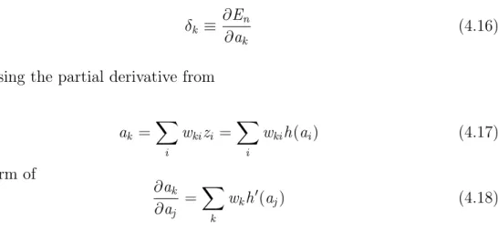
δk ≡ ∂En

∂ak

(4.16) and using the partial derivative from

ak = X i wkizi = X i wkih(ai) (4.17) to the form of ∂ak ∂aj =X k wkh0(aj) (4.18) we arrive at the backpropagation formula for error derivatives at stage j.

δj =h0(aj)

X

k

wkjδk (4.19)

Equation (4.19) denotes that the value of δ for a particular hidden neuron can be obtained by propagating the δ’s backward from neurons higher up in the network [26].

Figure 4.6: Flowchart illustrating how the backpropagation technique works. The blue arrows defining the forward flow of information and the red one’s backward flow. For simplicity sake, the biases were omitted.

The backpropagation algorithm is iterated through all the neurons until the value of the error function becomes sufficiently small. This repetitive cycle is known as an epoch. One epoch is equal to one forward pass and one backward pass through the entire training set[28]. A posing challenge of the learning phase

5

|

Deep Learning

During the last few decades, neural networks played a fundamental role in push-ing forward advancements in computational tasks such as speech recognition, image recognition and other. Continuous research in neural networks and a vast increase in available training data lead to the development of even more com-plex neural structures, from which the term Deep Learning emerged [29]. Neural networks which were described earlier in this paper present a shallow (3-layers) architecture of the network and their performance is significantly limited. Deep architectures with many hidden layers can execute more instructions than shal-low neural networks and outperform them in many important pattern recognition applications [30]. Deep neural networks (DNN) can train a large number of pa-rameters from the input data very efficiently. The extra provided layers also allow feature extraction and transformation which is very beneficial for complex prob-lems such as computer vision or natural language processing [31]. Fundamentally, the concept of DNNs is that the input data represent a value composed of several levels of abstraction, from simple concepts to complex. The networks are designed hierarchically extracting higher features from lower features [32].

5.1

Recurrent Neural Networks

As we introduced in section 4.2, artificial neural networks take an input in a sin-gle time period and work in a feed-forward motion. Fundamentally ANNs are not able to recognize the context of the problem because they form acyclic graphs. Recurrent neural networks are a modified class of ANNs that have feedback con-nections in order to store recent representations of inputs events. Simply speaking, they feed the output value or signal back into its input along with some sequence. This characteristic enables RNNs to exhibit dynamic behavior presenting its in-ner state or memory. Therefore allowing us to model long-term dependencies in sequential data which is suitable for times series modeling.

Chapter 5. Deep Learning

Figure 5.1: The straightforward diagram presents a recurrent cell. It takes in an input xt and outputs a valueht of the hidden layer in time t.

where Whx and Whh are weight matrices. Whx is the weight matrice between

the input and the hidden layer and Whh is the weight between the hidden layer

itself. Vector bh denotes the bias vector andf is the activation function [33]. The RNN returns one output yt at each time step accordingly:

yt =f(Whyht +by) (5.2) Why is the hidden to output weight matrice andht is the output of the hidden layer at time t.

Figure 5.2: Unrolling of RNN dynamics.

It is common practice to reveal the dynamic of RNN by unrolling as seen in Figure 5.2. This interpretation of the unrolled networks shows a very deep neural network with one layer per time step with fixed weights. So we can conclude that the unrolled RNN can be trained with backpropagation across many times steps. Although RNN are very efficient algorithms they have difficulties learning long sequences due to the vanishing gradient problem [34]. During training with backpropagation, the computed errors are multiplied by each other every step causing the gradient to grow too small, causing the network to learn only short-term relations. This issue is addressed by a novel recurrent network architecture called Long Short-Term Memory.

Chapter 5. Deep Learning

5.1.1

Long Short Term Memory - LSTM

RNN networks in principle use their feedback loop connections to store a rep-resentation of values from inputs in forms of activations. As mentioned in the previous section, RNN suffer from the vanishing gradient problem, where the er-ror signals tend to either vanish or extremely diverge. This issue was approach by Hochreiter and Schmidhuber [35] who introduced the LSTM model in order to tackle the problem of the vanishing gradient. The newly submitted model resem-bles the standard recurrent neural network but each node of this net is replaced with a new memory cell that can hold information for an arbitrary amount of time. The cell has a core unit called Constant Error Carousel (CEC) which is connected to a recurrent edge with a fixed weight one. This enforces a constant error flow ensuring that the gradient can pass several times without vanishing or diverging.

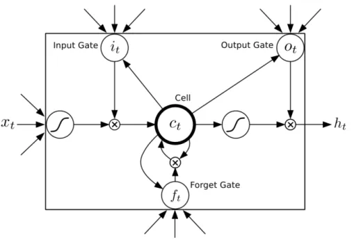
Figure 5.3: A scheme of a Long Short-Term Memory cell unit. The cell is struc-tured into four gates. TheInput Gate evaluates what values need to be updated. TheForget Gate calculates whether to keep the incoming information or not. The CEC Cell is responsible for preventing vanishing gradients. TheOutput Gate de-cides on the output [36].

Formally the process of calculating the output is more complex than in a standard RNN node, however, the principle of this operation derives from the same understanding. LSTM cells perform calculations of their outputsh at each

Chapter 5. Deep Learning

ct =ftct−1+ittanh(Wxcxt +Whcht−1+bc) (5.5)

ot =σ(Wxoxt +Whoht−1+Wcoct−1+bo) (5.6)

ht =ottanh(ct) (5.7)

i,f,o characterize input, forget and output vectors respectively. If the output

value is reaching 0 the gates block the information flow, on the other if the output value is close to 1 information will flow freely. Sigmoid and hyperbolic tangent tanh activation functions are used in the LSTM model [37].

6

|

Practical Implementation

6.1

Technical Background

The implementation part of the thesis is written in a dynamic, interpreted high-level programming language. The main features of Python that can be considered as an advantage compared to other languages include:

Readability - Python’s syntax is very clear and easy to interpret. It is unclut-tered, maintainable and resembles human written language.

Cross-platform - Python runs on all major operating systems like Microsoft, Linux, and Mac OS X. It is also open source with an active community of devel-opers further enhance it.

Extensive Library Support - The main advantage of Python stems fro its large variety of existing libraries. These libraries contain over 130 000 packages that provide tools suited for many tasks such as database handling, automation, web scraping, scientific computing, image processing and others [38]. Some of the li-braries, which I shall describe below, were selected and used for the task of this thesis. The code was written and executed in Jupyter Notebook a web-based, in-teractive environment supporting visualization, data analysis, and statistic mod-eling. Finally, Python is widely used for machine learning tasks and regarded as the most convenient language for this purpose.

As stated earlier, I will briefly introduce the libraries that were applied in the code leading to the solution of the problem at hand.

Numpy is a scientific library serving as the backbone for data

manipula-tion. It provides a large pool of mathematical functions, support for large, multi-dimensional arrays and matrices. It can be further adopted as an efficient con-tainer of generic data [39].

Pandasprovides high-performance tools for handling data structures,

numer-ical tables, time series and effective data reading [40].

Scikit-learnis a machine learning library featuring several effictient tools for

data analysis, data mining, supervised and unsupervised algorithms. It further 26

Chapter 6. Practical Implementation

contains packages for data visualization. We mainly use the data prepossessing packages in our work. [41].

Keras is an open source research library for deep neural network learning

applications. It provides a clean and efficient way of creating a wide range of neural network models on top of either Tensorflow1 _{and Theano}2 _[44].

TA-Lib is a large library specifically developed for trading professionals and

developers. It covers over 200 technical indicators, such as Relative Strength In-dex, Moving Average Convergence/Divergence and enables candle stick recogni-tion from datasests [45].

6.2

Data Analysis

In the first section, we shall introduce a fundamental overview of data and a brief analysis of the data in the cryptocurrency market. The second stage of this section will describe the chosen dataset for the problem and what steps need to be taken for implementation.

6.2.1

Data Fundamentals

Among several technical advancements introduced over the years, data followed along as a definite product of the modern economy. Data is generated by a di-verse array of actors such as sensors, computers, machines, government bodies, institutions, and people. In a general manner, data present an informative value of a given subject. Data is measured, collected and visualized in several forms for example logs, databases, and flat files. In our study we focus on financial data, particularly market data - see tbl.

The World Wide Web enabled an enormous surge of data being produced every day. This data is labeled as raw data and is usually unorganized and stored in data servers or individual hard disks. A collection of data is referred to as a data set which lists several variables and their values. Data sets can be of very large sizes shifting them into the realm of so called Big Data. An important attribute is data granularity which defines the size and how detailed the datasets are. In the area of financial forecasting, granularity plays a fundamental role. It can be considered as a parameter of the dataset with the property of possibly enhancing the accuracy of the model outcome. Datasets are either coarse-grained or

fine-Chapter 6. Practical Implementation

Figure 6.1: In our thesis, we work with Market Data as seen in the table - The Four Essential Types of Financial Data [46].

Cryptocurrencies are a very recent occurrence in comparison to other assets in the financial markets. Although Bitcoin was invented in 2009, it’s relevance as a trading asset is significant mostly from the year 2013. The amount of data is therefore limited to only a few years. The market experienced considerable turbulence’s as well as an increase in the amount companies issuing their own cryptocurrency. Like with almost any data analysis problem a subject of research is - how accessible and in what quality is the data available. Cryptocurrencies present an advantage in this state because their market data is significantly more available than data of traditional FX currencies. Exchanges offer their API’s for the collection of live data in the form of json files. Better established exchanges provide historical prices in the form of OHLC (Open-High-Low-Close) as well as high-frequency data. The market has highly disintegrated prices across all the exchanges in the space; this may potentially provide an opportunity for testing the effectivity of our strategy. It is therefore critical to train and test the algorithms on a dataset from retrieved from one exchange.

On the other hand, analyzing datasets from several exchanges can provide better insight into the current situation on the market. Another drawback lies in the fact that the freely available datasets with desirable characteristics are mostly available for Bitcoin in contrary to altcoins3_{. Cryptocurrency exchanges}

are open every day of the year and seasonality is not evident. They also differ in the trading fees - some have a uniform price, others do not charge trading fees. The market experienced incredible growth from the second quarter of 2017 to the first quarter of 2018 before encountering a correction. This vast influx of capital into the market led to an increase of thousands of percent of all cryptocurrency prices. Due to this evolution, we should consider two approaches: an analysis of the market before the major inflation and an analysis from the time period of 2014 to 2017.

3_{Altcoins are alternative cryptocurrencies that emerged from Bitcoin. They are} fundamen-tally based on the Bitcoin protocol but differ in some technological aspects [47].

Chapter 6. Practical Implementation

In this section, we described the most relevant theoretical concepts of data and data analysis. Furthermore, we examined the cryptocurrency market and its setting in data science.

6.2.2

Data Processing

The process of data analysis and processing requires knowledge of the presented problem. A variety of tools and methods that are feasible today provide an excel-lent asset in preparing the datasets for further use. But the developer might still need to apply manual techniques and proceeds in order to achieve a functional dataset. So In this subsection we shall go through the process of collecting the data, describing the main characteristics, cleaning it and processing it into a form suitable for our prediction model.

6.2.2.1 Data Collection

Due to the nature of the cryptocurrency market consisting of severe fluctuations throughout the day, we came to a conclusion that a dataset with a granular-ity level of one-minute intervals presents a good alternative. The price percent-age change occurring on the cryptocurrency market increases dramatically over longer time periods, while on smaller scale intervals the fluctuations aren’t so significant. The logic behind this statement provides an argument for the usage of the mentioned dataset and granularity level. We collected four datasets from the exchange Bitfinex4 containing a time series of one-minute prices of Bitcoin

(BTC), Ethereum (ETH), Litecoin (LTC) and Bitcoin Cash (BCH) against the USD. Tha datasets contain no headers and the time feature is provided in a unix timestamp format. We converted the timestamp to a datatime format and added headers for illustrative purposes, see Table 6.2. All of the datasets initialize on the 2018-06-14 ; 09:31:00 and finish on the 2018-08-25 ; 16:37:00. Raw trading data comes in several variations with different indexes and values adjusted to them. In our case, the order of features is changed from the commonly known OHLC. This is not an issue as we will feed our prediction model only the Close values.

We eventually need to drop all of the empty values NaN located in the sets. The collected and cleaned dataset will be used to train and test the price prediction models.

Chapter 6. Practical Implementation

• Open: Opening price of the cryptocurrency at the start of trading. Doesn’t

need to correspond to the closing price • Close: Closing price at the end of trading

• Volume: The total quantity of traded tokens or coins over a time period.

Time Low High Open Close Volume

2018-06-14 09:31:00 96.580002 96.589996 96.589996 96.580002 9.647200 2018-06-14 09:32:00 96.449997 96.669998 96.589996 96.660004 314.387024 2018-06-14 09:33:00 96.470001 96.570000 96.570000 96.570000 77.129799 Table 6.1: Table with historical price data. This example shows the LTC-USD dataset

Because the dataset is virtually a sequence of time series data points, or in-herently sequential, we need to restructuralize so as to prevent fromoverfitting5_.

6.2.2.2 Data Normalization

It takes several steps before the dataset can be fed into the model. One of them is to normalize the data. Fundamentally what we are trying to achieve with normal-izing the data is to scale them into a range easily interpretable for the network. By normalizing we rescale the data from (e.g. 10s to 100s value) into values on the scale of [-1, 0, 1]. Without this scaling, the widely different feature values might cause the fed model to create a bias and adjust weights unevenly leading onto slow and possibly inaccurate training. On of the approaches of normalizing the data is to apply MinMaxScaler provided by Keras. This method ensures that the dimensions of the input features are in the borders of [-1, 1] without the leakage of outliers [50]. By doing so we managed to smooth out the training data for the model and fit the input features into an appropriate scale for the activation function.

6.2.2.3 Training and Testing Data

After cleaning and normalizing the data we have to determine what fraction of the dataset should be reserved as a training set and what section as the testing set. Given the non-stationarity of cryptocurrency prices, we face a dilema; using too much data for training will make our model irrelevant, using too little data for training will most likely lead to underfitting6 _{of the model. One might therefore}

ask, what is the ideal ratio of training to testing data? The answer to this question 5_{"The production of an analysis which corresponds too closely or exactly to a particular set} of data, and may fail to fit additional data or predict future observations reliably" [49]

6_{The opposite issue of overfitting - definition stated earlier} 30

Chapter 6. Practical Implementation

is not straightforward but a theory built on other real life problems addresses this issue most frequently. It states that from any event, about 80% of the effects come from 20% of causes [51]. This theory is called thePareto principle. For our purposes, we decided to split the dataset into a ratio of 80% training data and 20% testing data, supported by research on this topic [52].

Figure 6.2: Graph showing normalized input feauture - close price. Cryptocurreny pair LTC/USD.

Figure 6.3: Graph indicating the ratio of 80% to 20% of training/testing data. In this chapter, we described the fundamentals of data and datasets. What are

Chapter 6. Practical Implementation

6.3

Methodology

6.3.1

Motivation

The motivation behind choosing the topics of prediction cryptocurrencies with machine learning algorithms was heavily inspired by the increasingly better per-forming neural network architectures. With widespread media coverage of cryp-tocurrencies during the year 2018 the public began to question this speculative security but also began to comprehend machine learning techniques and challenge biases associated with predicting future asset prices. The community of develop-ers interested in both cryptocurrency technology as well as machine learning grew taking me along. Neural networks are a tool applied on time series for prediction purposes for several decades with mediocre results. During the last few years, the amount of freely available data increased dramatically and other algorithms could be tested and improved upon. Applications desiring the use of machine learning algorithms increased and most of them work very efficiently. Recurrent Neural Networks proved to be a good bet on the use of forecasting time series but it lacked the ability to handle the vanishing gradient problem. Long Short-Term Memory cells suppressed this problem. This characteristic proved to be a useful asset in asserting time-series tasks, especially thanks to their ability to find non-linear relationships among the data over a sequence of time. They are also suitable for this task due to the memory state giving them the edge of understanding tem-poral dependencies. The strong results of LSTM networks on predicting future prices support our motivation to build a predictive Recurrent Network model as well.

6.3.2

Technical Indicators as Features

Recurrent networks with LSTM cells are capable of reaching good results using only the normalized inputs and activation function. On the other hand technical indicators - tools developed in the 20. century precisely for the financial markets can enhance the results obtained by RNN alone.

Technical indicators are mathematical calculations building on domain knowl-edge from technical analysis. While technical analysis builds on a wide range of different methods and techniques, we will focus on applying the most popular features. For our task, we used the Simple Moving Average, Standard Deviation and Relative Strength Index as enhancing input features.

Chapter 6. Practical Implementation

closing prices recorded over a time period, divided by the total number of prices in the calculation. So, for instance, a 15-day moving average is the result of the last ten closing prices divided by ten [53]. We have constructed three moving averages in the range of 15-minute, 30-minute and 60-minute.

Figure 6.4: Depiction of the Simple Moving Average feature. The image clearly shows how reactive the individually set MA are to price changes. This graph depicts the first 600 minutes of trading.

Standard Deviation

Another technical indicator that we use as a feature is the Standard Deviation (STD). It measures the amount of variability or volatility relative to the moving average. The higher the standard deviation, the higher the volatility in that given time period. it is a useful tool specifically in the cryptocurrency market because it indicates the possible future price volatility rate. A simple rule is that if the STD is too low the market is absolutely inactive and we can expect rapid change. If STD is too high a decline in activity might occur [54].

Relative Strength Index

The Relative Strength Index (RSI) is a momentum indicator for analyzing the current and historical index or speed and change constructed from occurred price changes over a certain period of time. The RSI oscillates between the values of 0 and 100. Developed by J. Welles Wilder [55] who stated that if the RSI values are in the range of 70, the security is considered overbought. When the RSI range is at around 30 it is considered to be oversold. This is an excellent instrument for recognizing whether or not a cryptocurrency is pumped - overbought or dumped - oversold.

Chapter 6. Practical Implementation

Listing 6.1: A snippet of the technical indicator features coded in Python

import talib

import pandas as pd import numpy as np # Data Loading

Path = "~/LTC−USD.csv"

df = pd.read_csv(Path, names=["Time", "Low", "High", "Open", "Close", " Volume"])

# Simple Moving Average

df["15minute MA"] = df["Close"].shift(1).rolling (window = 15).mean() df["30minute MA"] = df["Close"].shift(1).rolling (window = 30).mean() df["60minute MA"] = df["Close"].shift(1).rolling (window = 60).mean()

# Standard deviation

df["STD"]= df["Close"].rolling(5).std()

# Relative Strength index

df["RSI"] = RSI(df["Close"].values, timeperiod = 9)

6.3.3

Sliding Window

Before we begin our simulations we need to define what steps are taken for the model to essentially learn to predict into the future. The dataset containing the closed prices is a time series of lengthN and with a closing price ofp0,p1, ...,pN−1.

Now with this in mind we can imagine a method, containing a sliding window represented by a variable Window and to which we assign a numerical value containing the information of how much to the right can the window slide. This practice is generally referred to as a method for partitioning or lagging method.

Listing 6.2: Python code for sliding window

#Sliding Window

defextract_window_data(df, window=15, zero_base=True):

window_data = []

for idx in range(len(df)− window):

Chapter 6. Practical Implementation

We began this chapter with a brief overview of neural networks in relation to future price predictions. We further discussed our motivation to research the effectivness of RNN for the problem of predicting the future price. Afterward, we followed up on technical indicators adopted as features for the RNN-LSTM network. And finally, we presented the sliding window method as our means of predicting the future cryptocurrency price.

6.4

Prediction Model Evaluation

This chapter examines the process of applying the price prediction strategy with analytically prepared data to the Recurrent Neural Network with LSTM cells. The prediction model was designed in accordance with common principles and with the use of the Keras library. The model’s performance will be evaluated and presented in the form of graphs and in a table with respect to its parameters.

6.4.1

Recurrent Network - LSTM

The first parameter for selection was the size of the sliding windowWt. Thanks to

the high level of granularity that the dataset contains we based the window size on a 15-minute time interval into the future. The values of the sliding window start at

W0 to the windowWt+15at timet. This parameter lies outside of hyperparameters

of the actual RNN-LSTM network.

6.4.1.1 Model Hyperparameters

Before the simulation was conducted a thorough grid-search was performed on the selected parameters of the prediction model. The grid search did not include windows size and training size, those values were chosen arbitrarily.

Optimizer

The stochastic gradient descent algorithm is an important element in Neural Network, specifically for updating network weights during training. Several other optimization algorithms have been developed and applied in machine learning algorithms. We have adopted a new algorithm named Adam. This optimizer is suitable for non-convex optimization problems and has a list of beneficial aspects, to name a few: little memory requirements, effecient for problems with noisy gradients, computationally efficient etc.[56].

Chapter 6. Practical Implementation

Batch Size

Batch Size is simply put a the number of samples that will be propagated through the network during the training phase. It’s size directly correlates with the amount of memory used for training. The higher the batch size, the more memory is used.

Epoch

An epoch is a term used for the number of training cycles the training set. One epoch is equal to one forward and backward pass through the network.

Dropout Probability

Dropout probability is a method of regularizing a neural network. Its a tech-nique to reduce the chance of overfitting by randomly selecting and setting some neurons to zero. Dropout is used only during the training of the network. A rule of thumb is to set the dropout value to about 25% of the total amount of neurons [57].

Window Size #Hidden Layers Neurons

15 1 64

Batch Size Activation Optimizer

32 Linear Adam

Epochs Dropout Probability Loss Function

15 0.25 MAE, MSE

Table 6.2: Parameters settings of the RNN-LSTM model that yield the best results.

Chapter 6. Practical Implementation

6.4.2

Results

In this subsection we shall present and go over the performance results of the prediction model. We obtained four cryptocurrency datasets, containing OHLC features of Litecoin, Bitcoin, Ethereum and Bitcoin Cash with one-minute time-stamp intervals. For evaluating our prediction model, we applied two metrics that measure their predictive accuracy per se;Mean Absolute Error (MAE) and Mean Squared Error (MSE)[58].

MAE = 1 n n X i=1 |yi −ˆy | (6.1) and MAE = 1 n n X i=1 (yi −ˆy)2 (6.2) After receiving the prediction values from the backtest, we had to denormalize the data. The real closing price of the currency pair LTC/USD is pictured as a blue line, the model’s prediction as an orange line, see Figure 6.5.

Figure 6.5: Denormalized close price data against the prediction of the currency pair LTC/USD.

The Figure 6.5 indicates that the prediction model has performed seemingly well on on unseen data of the closing price of LTC/USD. Predictions of the Litecoin price in USD is plotted over a time frame of 600 minutes in 15 minute time-steps.

Chapter 6. Practical Implementation

Figure 6.6: A detailed look on the denormalized close price against the prediction of the currency pair LTC/USD. The graph is a 120 minute time frame in 15 minute time-steps.

Figure 8.8 is better suited for a closer examination of the models performance. Even on a finer scale, we see that the accuracy is good but after a deeper analysis it is relatively clear that the model is able to access the source of error and adjust itself accordingly. An obvious flaw is detectable in the sudden price spikes. Even moderate changes in the closing price tend to pose an issue for the model. This is a persistent failure of the model throughout the entire testing set. In the stable areas the model seems to behave in accordance with the real closing price. Overall, by drawing a conclusion from the graphical results we can say that the model is decent in predicting on unseen data.

Chapter 6. Practical Implementation Evaluation Metrics

LTC/USD

Mean Absolute Error (MAE) Mean Squared Error (MSE) Train Loss Test Loss 0.000830 2.71655e-06 0.000625 0.000830

BTC/USD

Mean Absolute Error (MAE) Mean Squared Error (MSE) Train Loss Test Loss 0.000662 2.28875e-06 0.000735 0.000662

ETH/USD

Mean Absolute Error (MAE) Mean Squared Error (MSE) Train Loss Test Loss 0.001150 4.51608e-06 0.000735 0.001150

BCH/USD

Mean Absolute Error (MAE) Mean Squared Error (MSE) Train Loss Test Loss 0.0012592 5.78892e-06 0.000999 0.0012592 Table 6.3: The table exhibits the numerical results of the prediction model. We present four metrics, MAE, MSE, Train Loss and Test Loss.

Apart from concluding a general view of the performance of the prediction model, we also yielded numerical results from problem-specific evaluation met-rics. The aforementioned metrics, specifically MAE and MSE measure the pre-diction accuracy. MAE evaluates the absolute value of the difference between the predicted value and the actual value, in our case real price. MSE is the squared metric. The smaller the calculated value of these metrics the better performing the prediction model. In our case, the values are exceptionally good, stating that the predicted values were rather close to the target closing price. The metric re-sults for Litecoin and Bitcoin are clearly analogous compared to Ethereum and Bitcoin Cash. All the datasets were applied on the same prediction model with the same parameter setting, so the cause of the significant invariance leeds to possible issues in the datasets. Therefore a more accurate approach in analysis the data might be needed.

According to our results of the prediction model, we can conclude that the strategy, data analysis and parameter settings proved sufficient enough to achieve good results overall. Though there is room for improvements, so to summarize:

• Better results could be obtained by creating or using a well adjusted pa-rameter optimizer.

• Applying a different strategy.

• Getting better and especially more data to train on.

• Selecting more cryptocurrencies or different cryptocurrencies. • Using different statistical measures

• Applying a different RNN architecture or algorithm - ANN, Random Forests

Chapter 6. Practical Implementation

In this chapter we concluded our findings and examined the performance of our prediction model. We applied two metrics that are most suitable for the evaluating the accuracy of a forecasting model. Eventually we outlined possibilities on how to improve the performance of the model. chapter 8 contains the rest of the simulations in the form of graphs.