Workload Characteristics of DNA Sequence Analysis: from Storage Systems Perspective

(1)

Workload Characteristics of DNA Sequence Analysis: from

Storage Systems’ Perspective

Kyeongyeol Lim, Geehan Park,

Minsuk Choi, Youjip Won

Hanyang University

17 Seongdonggu Hangdangdong, Seoul, Korea

{lkyeol, pghsky, 0310cms,

yjwon}@hanyang.ac.kr

Dongoh Kim, Hongyeon Kim

Electronics and Telecommunications Research

Institute

305-700, Daejeon, Korea

{dokim, kimhy}@etri.re.kr

ABSTRACT

The recent development of NGS (Next Generation Sequenc-ing) methods has greatly increased the amount of genome data and created the need for high-performance computing and high-performance storage systems. The key issue in developing high-performance storage systems is building a storage system that is optimized for NGS analysis pipeline. In this paper, we implemented a tool to collect and analyze I/O workload in NGS analysis pipeline. Using this tool, we executed NGS analysis pipeline and analyzed the character-istics of I/Os collected in the experiment.

Categories and Subject Descriptors

C.4 [Performance of Systems]: Measurement Techniques; D.4.8 [Operating System]: Performance—Measurements

General Terms

Design, Measurement

Keywords

Bioinformatics, I/O Workload analysis

1. INTRODUCTION

The human genome consists of DNA sequences and con-tains over three billion DNA base pairs. DNA sequences vary by ethnicity groups and by individuals. Variations in DNA sequences can be different types and sizes. The variations may represent genetic characteristics or may indicate a cause for genetic diseases. Genome analysis techniques analyze genetic structural variations, which are variations in DNA sequences. The types of variations include SNP (Single Nu-cleotide Polymorphism), Indel (Insertion and deletion), and CNV (Copy Number Variation).

A NGS analysis pipeline is a list of analytical steps and tasks that need to be followed in genome analysis. These

Permission to make digital or hard copies of all or part of this work for personal or classroom use is granted without fee provided that copies are not made or distributed for profit or commercial advantage and that copies bear this notice and the full citation on the first page. To copy otherwise, to republish, to post on servers or to redistribute to lists, requires prior specific permission and/or a fee.

RAPIDO’14, January 22 2014, Vienna, Austria

tasks include aligning sequences, identifying variations, an-alyzing the structure, etc. and they are executed in order.

The Human Genome Project successfully produced the first complete sequences of individual human genomes. This brought heightened interest in the diagnosis and treatment of diseases through genome research but the high cost associ-ated with the existing genome analysis technique was an ob-stacle. The recent development of Next Generation Sequenc-ing (NGS) enables high-throughput sequencSequenc-ing at a lower cost. With the existing, traditional sequencing technique, it takes about 34 years and 300 million dollars to sequence a human genome, consisting of three billion DNA base pairs. NGS techniques improved the speed of sequencing by 200 times and cost only 350,000 dollars[13]. Recent advance-ment in NGS techniques greatly increased the amount of genome data and created the need for high-performance computing and high-performance storage systems. Cloud-based genomics tools, such as CloudBurst[11], [5], and Myr-naCrossBow[4], are being researched as a solution. These tools allow executing analysis in parallel in each cluster. They use MapReduce[3] based distributed systems, such as Hadoop[2].

Although developing a storage system optimized for NGS analysis pipeline has become a very important issue, it is still not being extensively researched. In this paper, we imple-mented a tool to collect and analyze I/O workload of NGS analysis pipeline. We executed genome pipeline, using this tool, and characterized I/Os collected from the experiment. In Section 2, the characteristics of each step of NGS anal-ysis pipeline and the applications used in the steps are ex-plained. The implementation of workload analysis tool is described in Section 3. In Section 4, I/O workload col-lected from an actual NGS analysis pipeline is analyzed. Our conclusion and future research directions are summarized in Section 5.

2. NGS ANALYSIS PIPELINE

NGS analysis pipeline[1, 8, 10] consists of tasks related to identifying SNP information from genomic data and an-alyzing variations in the DNA sequences to extract disease related information. These tasks can be categorized into DNA sequence alignment step and SNP calling step. There are various applications that can be used in NGS analysis pipeline; in this paper, we used BWA[6] in DNA sequence alignment step and SAMtools[7] in SNP calling step.

(2)

Client Server Viewer Manager Web Interface Database iotrace module (FUSE) App lic atio n TCP/IP PH P, JSO N iotrace module (FUSE) iotrace module (FUSE)

Figure 1: System Overview

This step consists of two sub steps: First is bwa aln

step, where we create index from the human reference genome using BWT (Burrows-Wheeler Transform) al-gorithm[6] and create SA (Suffix Array) information from the index. Second isbwa sampe step, where we use the SA information from the first step to coor-dinate DNA sequence with the reference and convert the information to SAM (Sequence Alignment/Map) format[9]

• SNP calling step

This step consists of the following 7 steps. (i)

sam-tool view: SAM/BAM format data is extracted from

the sequencing results, (ii)samtool sort: the mapping results in BAM format are aligned with the reference sequence, (iii)samtool index: index is created to allow fast look-up of data in SAM/BAM files, (iv) samtool flagstat: statistical information is extracted from the results of alignment, (v)samtool merge: BAM format files are merged, (vi)samtool mpileup: from BAM for-mat files, variations are produced in BCF (Binary Call Format) files, and (vii) bcftools: the final output are produced in VCF (Variant Call Format) files.

3. WORKLOAD ANALYSIS TOOL

3.1 Overview

In this paper, we developed a tool to analyze I/O work-load of NGS analysis pipeline. This tool supports multi-client environment and is not restricted to one specific file system. Fig. 1 illustrates the structure of the workload anal-ysis tool; it consists ofiotrace module, aanalysis server, and

WebGUI. iotrace module exists in each client as an agent to support multi-client environment. It is implemented on FUSE (Filesystem in Userspace)[12]. Traces of I/O requests from each client’s NGS analysis pipeline are collected by io-trace moduleat the file system level. They are transmitted to the analysis server through TCP/IP. Theanalysis server

collects the I/O data received, then analyzes and saves the data in the database. The workload information is man-aged and monitored in the analysis server using WebGUI.

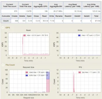
WebGUI provides real-time monitoring for various types

of I/O information. Upon completing workload analysis, the system provides analysis results and statistical informa-tion, including execution time for each step of NGS analysis pipeline, various access patterns, IOPS, bandwidth, file ac-cess frequency, the number of requests by request size, CPU

Figure 2: WebGUI

utilization, etc (Fig. 2).

3.2 Tracing Techniques to Collect I/O Data

There are a number of techniques available to collect I/O workload tracing data. Adjusting the kernel’s system call to collect the data is one way. I/O data at the system call level can be collected by using strace, or at the block level by using blktrace. Network traffic data can be collected using tcpdump trace.

Adjusting the kernel’s system call to collect the data has an advantage of not incurring additional overhead but it is difficult to implement and is restricted to the kernel’s ver-sion which means the system needs to be revised when the kernel’s version changes. Using strace does not incur addi-tional overhead and is easy to implement. However, it can only collect workload data from one process and its child processes which makes it difficult to use it for real-world workloads. blktrace enables I/O data collection at the block I/O level without additional overhead; however, this does not fit our goal of collecting the data at the file system level. In this paper, we implemented trace module using FUSE file system. FUSE based trace module is implemented in-dependent of the kernel and, therefore, is not affected by changes in the kernel’s version. It can also be used inde-pendent of the file system. However, having an additional layer of FUSE module in the user space before the native file system may decrease the system’s overall performance.

3.3 I/O Trace Module

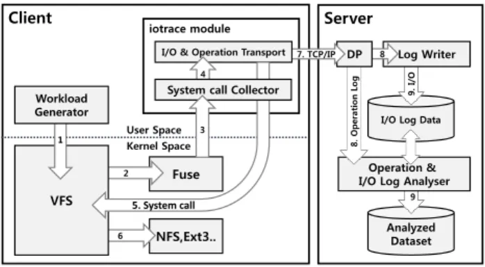
I/O trace module is one of the most important aspects of the workload analysis system. It exists in each client, where the actual workloads are being executed, as an agent and is implemented on FUSE. Fig. 3 shows the process of collect-ing the trace data of I/O requests created by the workload generator. First, I/O requests are created by the workload generator, such as NGS analysis pipeline or Iozone. Then, the I/O requests call native file system functions in FUSE based file system functions through VFS and FUSE module.

(3)

Server

I/O Log Data

9. I/ O Log Writer 8 Client iotrace module Analyzed Dataset User Space Kernel Space 9 Operation & I/O Log Analyser

8. Op era ti on L og DP 7. TCP/IP Fuse 2

I/O & Operation Transport

NFS,Ext3.. 6 VFS 1 Workload Generator 4 5. System call

System call Collector 3

Figure 3: Flow Diagram

collector_open(const char *path , struct fuse_file_info *fi ) { io_info_t io_info; … fd = open(path, fi->flag); … io_capture(&io_info) … }

open (“/mnt/collector/tmp/testfile”, O_RDONLY )

IO Capture Target Application

iotrace

EXT4,…

Figure 4: I/O Information Capture Function Table 1: I/O Information Collection Structure

typedef struct io info io{ int op code; // operation code int name len; // full path length int count; // operation count size t size; // request size

struct timeval latency; // latency time int pid; // process ID

int fd; // file descriptor

struct timeval open start time; // open index unsigned int client ip; // Client IP

struct list head offset head; // offset list head struct timeval start time; // timestamp(start time) }io info s t;

Upon completing the native file system functions, I/O data collecting function gathers information such as I/Os’ execu-tion time, request size, etc. (Fig. 4). The collected I/O data is transmitted to theanalysis server through TCP/IP.

3.4 Collected Workload Data

I/O data contains various file system call status, includ-ing read, write, create, unlink, open, close, etc. The I/O data collected for a specified time period is transmitted to a

analysis server. The server then saves the received workload data in the database. All workload data is either transmit-ted to theanalysis server in real-time or saved in the local client, where the workload is created, as a CSV (Comma Separated Values) file as needed.

Analysis Server DB thread1 DB thread2 DB thread3 DB threadn C ommuni cation Mo dul e Client Client Client Client Client Epoll thread1 Epoll thread2 Epoll thread3 Epoll threadn

. . .

... ... Log Queue Client1 Client2 Client3 Clientn

Figure 5: Server Configuration Table 2: Data Set

Count File size Human reference genome 10 11GB Human whole genom sequencing data 14 218GB

Table 1 is I/O data collection structure to gather file sys-tem call data. op code determines the type of a system call. The number of I/O requests collected is stored in count variable. Request volume size is stored in size vari-able. start time stores the time at which the request was created. latency stores time it took for the I/O request to be processed. To allow look-up of the open operation cor-responding to the target read/write request, the timestamp of open operation is recorded in the request’s record.

3.5 Multi-Client Support

Fig. 5 shows the configuration of theanalysis server. Epoll threads in the analysis server check the server’s TCP buffer for any data received from the client through TCP/IP. If there is data received, the tread brings the log information of I/O workload and pushes it to its own queue. DB threads check their queue for any assigned information. If there is information assigned, the DB thread pops the log infor-mation from the queue in the order received and saves it in the database. This saving process is performed multi-threaded which may cause problems with sequencing be-tween the queues. Also, there exist dependencies among workload data. To solve this problem, a dependency test is performed before DB thread saves workload information to the database. If an error occurs, the information is inserted back in the middle of the queue.

4. EVALUATION

4.1 Experiment Setup

The human genome contains over three billion DNA base pairs. When DNA sequencing is done with 10-40x coverage, the number of DNA base pairs becomes 30 billion to 120 billion. In this experiment, we analyzed about 500 million human genome sequence reads. We also included human reference genome data in the analysis. The size of the data set used in this experiment is shown in Table 2.

The test bed consists of one client, which executes NGS analysis pipeline, one NFS storage server, and one analysis server; all of which are connected with 10G network. All the data used in the experiment and the files created during

(4)

the process are saved in the NFS server. The client and the servers used in this experiment are Intel Xeon QuadCore E5620 2.4Ghz x 2ea, with 32GB memory, and 32 GByte SSD.

Table 3 shows NGS analysis pipeline configuration used in this experiment. NGS analysis pipeline consists of two main steps: NGS sequence mapping step and SNP calling step. BWA and SAMtools applications are used in NGS sequence mapping step and SNP calling step, respectively. For the analysis, the following commands were executed in the order listed: bwa aln, bwa sampe, samtools view|sort, samtools index, samtools flagstat, samtools merge, samtools index, samtools mpileup, and bcftools view. Most of these commands produce output files which are used as inputs for the next step. We categorized the commands into the following five groups for our analysis: bwa aln, bwa sampe, samtools sort, samtools merge, and samtools mpileup.

4.2 File operation summary

Table 4 is a summary of file operations and the informa-tion on files created and deleted in each step of the pipeline Overall, a total of 630 files, totaling 1031.7 GByte in size, were created; 535 files, 91.4 GByte in size, were deleted; and files were opened 4756 times. bwa sampe and sam-tools mpileup steps created files totaling 320.0 GByte and 323.4 GByte in size, respectively. Inbwa aln step, files were opened 2979 times and 91 GByte was created, indicating that this step produces small I/Os frequently.

4.3 Access Frequency

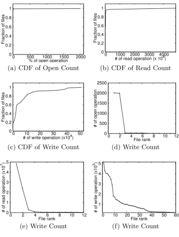
Fig. 6a, Fig. 6b, and Fig. 6c show the CDF of access fre-quency. In Fig. 6d, Fig. 6e, and Fig. 6e, we sorted files by their access frequency and showed the top 12 and 60 files. To review access frequency, we used the number of files opened (Fig. 6a and Fig. 6d) and the number of I/O requests (Fig. 6b, Fig. 6c, Fig. 6e, and Fig. 6f).

In read operations, we found that only a few files incurred most of the read requests. Of all files, the top 5% (31 files) constituted 99% of the total number of read requests. The top 0.3% (2 files) accounted for 80% of all read requests. By placing these 2 files in high performing SSD storage, we can expect to improve storage performance and reduce energy consumption.

In write operations, 9 files, the top 1.3% of all files, ac-counted for 75% of the total number of write requests. Only a small number of files produced most of the write requests, same as in read operations.

4.4 Access Pattern

Fig 7 shows the number of I/O requests by size in each step of NGS analysis pipeline. When one or more I/O requests are created sequentially, the sum of the requests’ sizes are shown on the x-axis. y-axis represents the number of times each I/O request size occurred. In bwa aln step and bwa sampestep, 96% and 83% of the total requests, respectively, were over 1 MByte in size. In samtools sort step, write requests over 1 MByte accounted for 97% of all write re-quests; however, the number of read requests in 4 KByte, 128 KByte, and over 1 MByte were all close. Insamtools merge

step, most write requests were over 1 MByte in size; read requests were mostly 512 KByte or over 1 MByte. In sam-tools mpileup step, most write requests were over 1 MByte and most read requests were 512 KByte. Overall, 94% of all

0 0.2 0.4 0.6 0.8 1 0 500 1000 1500 2000 Fraction of files % of open operation

(a) CDF of Open Count

0 0.2 0.4 0.6 0.8 1 0 1000 2000 3000 4000 Fraction of files # of read operation (x 104) (b) CDF of Read Count 0 0.2 0.4 0.6 0.8 1 0 10 20 30 40 50 Fraction of files # of write operation (x104) (c) CDF of Write Count 0 500 1000 1500 2000 2500 0 2 4 6 8 10 12 # of open operation File rank (d) Write Count 0 1 2 3 4 5 0 2 4 6 8 10 12 # of read operation (x10 7) File rank

(e) Write Count

1 2 3 4 5 0 10 20 30 40 50 60 # of write operation (x10 5) File rank (f) Write Count Figure 6: Access Frequency

0 2 4 6 8 10 12 14 16 18 4k 8k 16k 32k 64k 128k 256k 512k 1m 1m+ Counts (log2) Request sizes

aln sampe sort merge mpileup

(a) Read Count

0 2 4 6 8 10 12 14 16 4k 8k 16k 32k 64k 128k 256k 512k 1m 1m+ Counts (log2) Request sizes

aln sampe sort merge mpileup

(b) Write Count Figure 7: Request Size Count

(5)

Table 3: NGS Analysis Pipeline Configuration NGS sequence mapping SNP Calling

Application bwa samtools bcftools

Option aln sampe view|sort index flagstat merge index mpileup view Input .fastq .sai, fastq .sam .bam .bam .bam .bam .merged .bam .bcf Output .sai .sam .bam .bam.bai .flagstat .bam .bam.bai .bcf .vcf Term bwa aln bwa sampe samtools sort samtools merge samtools mpileup

Table 4: # of File Operation and Write/Delete File Size

# of Files Created/Deleted/Opend Write size (GByte) Delete size (GByte)

bwa aln 14/0/2979 91.0 0 bwa sampe 7/0/1647 320.0 91.0 samtools sort 556/535/12 227.0 0 samtools merge 2/0/10 69.4 0 samtools mpileup 52/0/108 323.4 0 total 631/535/4756 1031.7 91.4 0 2 4 6 8 10 12

seq. read seq. write rand. read rand. write

Counts (log2)

Pattern type aln

sampe mergesort mpileup

Figure 8: Access Pattern During File Open Table 5: Each File’s Access Pattern

Read Write R/W Pattern

bwa aln 18 12 2 bwa sampe 33 6 1 samtools sort 7 14 542 samtools merge 9 2 1 samtools mpileup 3 25 26 total 22 39 590

I/O requests were over 512 KByte in size.

Fig 8 displays the access pattern while files are open. If a file reads or writes sequentially from the time it is opened until it is closed, it is classified as ”sequential read/write”. If the offset changes out of sequence while the file is open, it is classified as ”random read/write”. In this experiment, most read requests were random and most write requests were sequential.

To analyze each file’s access pattern, we categorized files into read-only, write-only, and read-and-write as shown in Table 5. Inbwa aln step, both read pattern and write pat-tern existed equally. Inbwa sampestep, 82% of all files were read-only. Insamtools sort step, 92% of all files were

read-and-write. Insamtools merge step, there were 9 read-only files, 2 write-only files, and 1 read-and-write file. In sam-tools mpileup step, both write-only and read-and-write files were equally observed. For the overall workload, many files showed read-and-write pattern.

4.5 Bandwidth

Fig. 9 shows read/write bandwidth of NGS analysis pipeline workloads. The five steps in NGS analysis pipeline are marked by bold solid lines. In each step, the target ap-plication is executed repeatedly; the repetitions are divided by dotted lines. Each step displayed unique patterns. Inbwa alnstep, bandwidth showed high peaks which were produced by the top 2 files with the largest read request size. Inbwa sampestep, large amount of data was read and written con-tinuously in short time periods throughout the process. In

samtools sortstep, continuous read and write patterns were repeated at intervals. In samtools merge step, continuous write operations were displayed for the most of the period with a peak in read bandwidth at the end of the step. In

samtools mpileup step, there were few read operations but periodical peaks existed in write bandwidth, showing a write intensive pattern. Most of write operations occurred during

bwa sampe andsamtools mpileupsteps.

Fig. 9c is the CDF of read/write bandwidth. Write re-quests started inbwa aln step but most of them were ob-served inbwa sampeand samtools mpileup steps which have long execution time. Most of read requests were created in

bwa sampestep. Fig. 10 shows the CPU utilization for user, system, and iowait. Fig. 9a and Fig. 9b exhibit similar pat-terns to Fig. 10b and Fig. 10a, respectively. Fig. 10b shows that in bwa aln and bwa sampe steps, the CPU was used for a short period at a time and the usage was repeated at short intervals. samtools mpileup step showed the most CPU intensive pattern.

5. CONCLUSIONS

In this paper, we implemented a workload analysis tool for NGS analysis pipeline. Using this tool, we collected and an-alyzed I/O workload from NGS analysis pipeline and found that each step in NGS analysis pipeline displays unique I/O characteristics. Our experiment lasted 98 hours during

(6)

0 100 200 300 400 500 600 700 800 0 10 20 30 40 50 60 70 80 90 100 Bandwidth (MByte/Sec)

Snapshot time (Hour)

bwa aln bwa sampe samtools sort samtools

merge samtools mpileup

(a) Read Bandwidth

0 100 200 300 400 500 600 700 800 0 10 20 30 40 50 60 70 80 90 100 Bandwidth (MByte/Sec)

(b) Write Bandwidth 0 0.2 0.4 0.6 0.8 1 0 10 20 30 40 50 60 70 80 90 100 Fraction of requests

Read Write (c) CDF of R/W Bandwidth Figure 9: Bandwidth 0 20 40 60 80 100 0 10 20 30 40 50 60 70 80 90 100 Bandwidth (MByte/Sec)

merge

samtools mpileup

(a) CPU User

0 20 40 60 80 100 0 10 20 30 40 50 60 70 80 90 100 Bandwidth (MByte/Sec)

(b) CPU System 0 20 40 60 80 100 0 10 20 30 40 50 60 70 80 90 100 Bandwidth (MByte/Sec)

merge

samtools mpileup

(c) CPU iowait Figure 10: CPU Usage

(7)

which time, files totaling 1031.7 GByte in size were created and 91.4 GByte were deleted.

Of 631 files created, the top 2 files (0.3% of the total num-ber of files) accounted for 80% of the total access frequency. The 2 files are both in human reference genome data set. When we reviewed the access pattern by request size, we found that most read requests were over 1 MByte in size and most write requests were over 512 KByte. Most read requests were random and most write requests were sequen-tial.

Each step in NGS analysis pipeline exhibited a unique bandwidth pattern. bwa aln step showed read intensive pattern with periodical peaks in bandwidth. Inbwa sampe

step, large amount of data was continuously read or writ-ten in short time frames throughout the whole period. In

samtools sort step, continuous read and write patterns re-peated periodically. samtools mergestep showed continuous write pattern for the most part with a short and intensive read pattern at the end. Write requests were evenly spread throughout the analysis pipeline, starting in bwa aln step. Most read requests were produced inbwa sampe step. sam-tools mpileupstep showed a CPU intensive pattern.

For the future work, we plan to use currently available distributed file system, such as Hadoop, to collect and an-alyze the workload. Based on the information derived from the workload analysis, we intend to develop a consulting al-gorithm and system that can help us build a storage system optimized for NGS analysis pipeline.

6. ACKNOWLEDGMENTS

This work was supported by the IT R&D program of MSIP/ KEIT [10038768, The Development of Supercom-puting System for the Genome Analysis] and supported by IT R&D program MKE/KEIT. [No.10035202, Large Scale hyper-MLC SSD Technology Development].

7. REFERENCES

[1] C. J. Bell, R. A. Dixon, A. D. Farmer, R. Flores, J. Inman, R. A. Gonzales, M. J. Harrison, N. L. Paiva, A. D. Scott, J. W. Weller, et al. The medicago genome initiative: a model legume database.Nucleic Acids Research, 29(1):114–117, 2001.

[2] D. Borthakur. The hadoop distributed file system: Architecture and design. 2007.

[3] J. Dean and S. Ghemawat. Mapreduce: simplified data processing on large clusters.Communications of the ACM, 51(1):107–113, 2008.

[4] B. Langmead, K. D. Hansen, J. T. Leek, et al. Cloud-scale rna-sequencing differential expression analysis with myrna.Genome Biol, 11(8):R83, 2010. [5] B. Langmead, M. C. Schatz, J. Lin, M. Pop, and S. L.

Salzberg. Searching for snps with cloud computing.

Genome Biol, 10(11):R134, 2009.

[6] H. Li and R. Durbin. Fast and accurate short read alignment with burrows–wheeler transform.

Bioinformatics, 25(14):1754–1760, 2009.

[7] H. Li, B. Handsaker, A. Wysoker, T. Fennell, J. Ruan, N. Homer, G. Marth, G. Abecasis, R. Durbin, et al. The sequence alignment/map format and samtools.

Bioinformatics, 25(16):2078–2079, 2009.

[8] L. K. Matukumalli, J. J. Grefenstette, D. L. Hyten, I.-Y. Choi, P. B. Cregan, and C. P. Van Tassell.

Snp-phage–high throughput snp discovery pipeline.

BMC bioinformatics, 7(1):468, 2006.

[9] A. McKenna, M. Hanna, E. Banks, A. Sivachenko, K. Cibulskis, A. Kernytsky, K. Garimella,

D. Altshuler, S. Gabriel, M. Daly, et al. The genome analysis toolkit: a mapreduce framework for analyzing next-generation dna sequencing data.Genome research, 20(9):1297–1303, 2010.

[10] S.-H. Park. It based bioinformatics.kiise, 21(6):20ˆa ˘A¸S26, 2003.

[11] M. C. Schatz. Cloudburst: highly sensitive read mapping with mapreduce.Bioinformatics, 25(11):1363–1369, 2009.

[12] M. Szeredi et al. Fuse: Filesystem in userspace.

Accessed on, 2010.

[13] A. von Bubnoff. Next-generation sequencing: the race is on.Cell, 132(5):721–723, 2008.