Characterising, Explaining, and Exploiting the Approximate Nature of Static
Analysis through Animation
David Binkley
Mark Harman
Jens Krinke
Loyola College
King’s College London
FernUniversit¨at in Hagen
Baltimore MD
Strand, London
58084 Hagen
21210-2699, USA.
WC2R 2LS, UK.
Germany.
Abstract
This paper addresses the question: “How can animated visualisation be used to express interesting properties of static analysis?” The particular focus is upon static depen-dence analysis, but the approach adopted in the paper is applicable to other forms of static analysis. The challenge is twofold. First, there is the inherent difficultly of using animation, which is inherently dynamic, as a representa-tion of static analysis, which is not. The paper shows one way in which this apparent contradiction can be overcome. Second, there is the harder challenge of ensuring that the animations so-produced correspond to features of genuine interest in the source code that are hard to visualize without animation.
To address these two challenges the paper shows how properties of static dependence analysis can be formulated in a manner suitable for animated visualisation. These for-mulations of dependence have been implemented and the re-sults used to provide dependence visualisations of the struc-ture of a set of C programs. All animations described in the paper are also viewable on-line.
1
Introduction
This paper addresses the question
“How can animated visualisation be used to ex-press interesting properties of static analysis?” This question presents two related technical challenges and one obvious presentational challenge: how to depict the re-sults of an implementation of source code analysis that em-ploys animation in a paper. To address the presentational challenge the paper presents stills from the animations de-scribed, but all animations are also available on a comple-mentary web page located at
www.cs.loyola.edu/˜binkley/scam06.html
In addition, as an ‘experimental curiosity’, an example of one of the animations is available on the upper right hand corner of the paper as a flick-book animation. For optimal performance, this flick-book animation should be viewed on a single-sided version of the paper, though it renders adequately on the double-sided version of the paper in the proceedings. Flicking through the page corners from front to back reveals the animation that is used in the example discussed in Section 4.2. In the electronic form, repeated clicking on ‘next page’ also should give an impression of the animation.
The two related technical challenges that the paper ad-dresses are to animate the static and to do so in a mean-ingful, non-trivial, manner. That is, to exploit the potential of animation, it is necessary to find aspects of static analy-sis that change over time; seeking the dynamic within the static. Furthermore, while it might be possible to resolve this apparent paradox by animating somesuperficialaspect of the static analysis, this would be of little practical use. Rather, it is necessary to construct the analysis, and the an-imation that brings it to life, in such a way that interesting features of the animation correspond to interesting and im-portant properties of the source code. Furthermore, to be worthwhile, these important properties should be properties that could not be easily visualized without animation.
The essence of the thesis that lies at the heart of this pa-per is that the inherent approximate nature of static analysis can be used as the basis for a meaningful animated charac-terisation of the analysis. That is, static analysis typically employs a doctrine of safe approximation; in order to con-struct results that approximate answers to essentially unde-cidable questions, static analysis algorithms return answers that denote a safe approximation to the real (but generally undecidable answer).
For example, in pointer analysis, the set of identifiers to which a pointer variable may point cannot be precisely de-termined using static analysis [22, 32]. Therefore, pointer analyses [41, 43] return a safe approximation that contains
the true points-to set, but may contain ‘false positives’. De-pendence analysis [19, 23, 24] employs a similar safe ap-proximation strategy. It determines, not the true dependence relation between elements of a program, but rather, a weaker relation that is provably certain to contain the true relation. A similar doctrine of ‘safe approximation’ is adopted to other static analysis problems, for example constant prop-agation [10], calling context analysis [11, 28], and the con-struction of flow and call graphs [2, 21].
The increasing levels of approximation available to anal-ysis approaches (usually at the cost of increased computa-tional resource) form a suitable set of time series results, for which animation can be surprisingly illuminating. As the paper will show, such an ‘animation of approximation’ can yield more than mere insight into the effects of differing levels of approximation; it also imbues the analysis with an additional dimension of representation. This additional di-mension can be used to reveal complex semantic structures in the source code. These structures are dynamic by nature and so it would be hard to visualize them without animation. The necessarily approximate nature of static analysis, has recently led to approximation receiving such a warm embrace that some authors have even gone a step further: considering unsafe approximations [18, 27]. Such unsafe approximations may, despite their lack of safety, reveal im-portant and useful properties of interest. Both work on safe approximation in static analysis, and more recent work on unsafe approximation, provide a wellspring of potential plications from which the animation of approximation ap-proach may draw.
As a case study in the application of the animation of ap-proximation approach, the paper considers the well-studied problems of slice-based dependence analysis [13, 23, 42]. Specifically, the case study considers the problem of visu-alizing the effects of different levels of call depth on static dependence analysis. The results show the way in which the level of dependence grows with increasing call depth. This reveals interesting dependence structures in the pro-gram such as the movement of dependence clusters as well as their formation.
The primary contributions of the paper are as follows: 1. The paper shows that the necessarily safe–but–
approximate nature of static analysis can be visualized using animations that show increasing levels of preci-sion of analysis
2. The paper presents the essential characteristics of such a visualisation, illustrating with a case study that for-mulates a problem in static dependence analysis as a sequence of approximations of monotonically increas-ing precision.
3. The paper reports results from the implementation of this formulation of dependence and its associated
an-imation, presenting the application of the approach to 13 C programs, ranging from 1,744 to 13,188 LOC. The paper shows how interesting properties of the ani-mations are related to interesting properties of the pro-grams being animated.
The rest of this paper is organized as follows: Section 2 presents a general framework for animated visualisation of static analysis, while Section 3 illustrates the framework with the formulation of a specific animated visualisation of Call-Depth Dependence Analysis, implemented using pro-gram slicing. Section 4 presents results of an implementa-tion of Call-Depth Dependence Analysis applied to a set of C programs. Section 5 presents related work and Section 6 concludes with directions for future work.
2
Animated Visualisation of Static Analysis
This section sets out a framework for animation of static analysis in more detail. It defines the terminology used to describe an instance of the application of the animation ap-proach and defines the properties that such an instance may exhibit. These properties are characterised as those that are desirable in order to ensure that animation is both possible and meaningful and those that support certain forms of an-imation. First, some terminology is introduced that capture the foundations upon which the animation approach is built.1. Parameterization
There will be a parameter set, denotedπ, which defines the behaviour of the static analysis with respect to the approximation. These parameters form the description that characterises the nature of the approximation. 2. Approximation level
The result of an analysis for a particular instantiation of parameter values is not constrained: it may be, for example, a single numeric value, a set of values, or some form of data structure. For each possible instan-tiation of parameter values ofπthe static analysis will yield a potentially different result. The set of param-eter value instantiations used in the animation will be termed the ‘approximation levels’.
3. Animation as a sequence of stills
Animations are comprised of a sequence of ‘still im-ages’ (stills) that are displayed over a series of time steps to create the illusion of continuous motion. In the approach to animation introduced in this paper, each still will correspond to the results of the analysis for a single approximation level. This makes it relatively easy to form a relationship between analysis results and their corresponding animation.
4. Approximation System
The term ‘approximation system’ will be used to de-note the combination of parameter setπ, static anal-ysis formulation, approximation level set, and anima-tion. The goal of the animation is to provide a moving depiction of properties of the static analysis of a sub-ject program with respect to the approximation levels defined by choice of parameters inπ.
There are a number of properties that should be enjoyed by an approximation system, in order for the animation to be meaningful. These ‘desirable properties’ ensure that it will be easy to associate each approximation level with a suitable still of the animation. They also aim to establish a framework in which it is likely that the visual properties of the animation correspond to well-defined and interest-ing semantic structures, implicitly denoted by the sequence of approximation levels. The desirable properties of an ap-proximation system are
1. Multiplicity
Multiplicity is the most basic requirement of an ap-proximation system. An apap-proximation system is Mul-tiplicit if it contains more than one approximation level. Of course, for most animations, ‘more than one’ is unlikely to be construed to mean merely two differ-ent approximation levels; animations tend to rely upon a larger multiplicity. However, there may be situations in which an oscillating animation, showing merely two approximation levels may have value and so the defi-nition of multiplicity is so-constructed as to allow this. 2. Visualizability
An approximation system is Vizualizable if the analy-sis result of each approximation level is denotable by some value, derived from the outcome of the analysis, that can be visualized in some static graphic form. The nature of the value is left unspecified by the Visualiz-ability constraint: the value need not be numeric, nor need it be scalar, but it has admit static visualisation as a still. Without this property is will be impossible to translate the outcome of a particular analysis to some aspect of a still in an animation, so animation in the form introduced by this paper would be impossible.
3. Relatedness
An approximation system is related if there exists a well-defined relationship between the interpretations placed upon the different approximation levels. This property is important to allow some meaning to be placed on the animation. The animation uses the pas-sage of time to indicate a relationship between the dif-ferent choices of approximation level. Therefore, it should be possible to establish a connection between the passage of time and the approximation level. 4. Ordinality
An approximation system is ordinal if the set of ap-proximation levels can be ordered by a total ordering relation. This means that the results obtained from different approximation levels can be animated with animation order corresponding to approximation level. Ordinality subsumes Relatedness, since an ordering is, by definition, a relation. Clearly it would be most at-tractive to have an ordinal approximation system, since this naturally maps onto a sequence of stills in the ani-mation. However, there may be useful animations that merely respect the (weaker) Relatedness property. As well as these desirable properties, there are also other properties that an approximation system may possess and that naturally suggest particular forms of animation ap-proach. As research in this area progresses, it is likely that more such properties will be defined. The list below is an initial attempt to establish a starting point for research into the construction of a more complete list of properties.
1. Monotonicity
An approximation system is monotonic if the values that result from the analysis at different approxima-tion levels are either monotonically increasing or de-creasing in the ordering imposed by the Property 4 defined above. Monotonicity is desirable for ease of comprehension. Monotonic approximation results can be depicted in an animation that progressively moves across the screen (from left to right, for example). This can often add to the expressiveness of the animation. Monotonicity subsumes Ordinality and therefore Re-latedness.
2. Discreteness
An approximation system is discrete if the set of possi-ble values that can result from the analysis for each ap-proximation level are finitely enumerable. This prop-erty is useful because the stills in an animation are nat-urally pixelized. While it will be possible to visualize continuous approximation systems by digitization, it is more likely that discrete approximation systems will map seamlessly onto the stills of the animation. 3. Sharpness
An approximation system is sharp if, for all stills, S and associated approximation levels L, there exists a one-to-one (bijective) mapping between the pixel values in S and the individual components of the value produced by the analysis forL. Clearly, Sharp-ness subsumes DiscreteSharp-ness since each still contains a finitely enumerable set of pixels. In a Discrete approx-imation system every dot in every still of the anapprox-imation meanssomething concrete and well-defined in analy-sis of the program.
3
Animation of Call-Depth Slicing
This section usesCall depthk-truncated slicing, a form of approximate static interprocedural dependence analysis, to illustrate the animation approach for static analysis advo-cated in this paper. Ak-truncated slice applies a variant of k-limiting in the construction of an interprocedural slices. Informally, a k-truncated slice, for some chosen value of k, considers only up toklevels of call depth for called or calling procedures. This leads to a series of approximation levels based on choices of the parameterk. Note that this technique is different than k-limited context slicing [28], which is calling-context sensitive up to depth k and then becomes context-insensitive for larger call depths (and thus imprecise but safe). Ak-truncated slice is always context-sensitive but does not include anything beyond call-depth k(thus, it is precise but can be considered unsafe until the limiting value ofkis reached).
In terms of the framework for animation introduced in the previous section,k-truncating produces an approxima-tion system where the parameter setπis simply the choice of k. The approximation levels therefore correspond to choices of limiting valuesk, which determine the depth of procedure calls. Each still of the animation is visualized us-ing an Monotone Slice-size Graph (MSG) [9]. A MSG is a graph of slice size, plotted for monotonically increasing size. That is, slices are sorted according to increasing (non-truncated) slice size and the sizes are plotted on the vertical axis against slice number in sorted order on the horizontal axis.
The rest of this section formalizesk-truncated slicing, the MSG used in the animation, and finally considers which of the properties from Section 2 the animation has. It is well known that precise interprocedural slicing requires more than simple transitive closure of a program’s dependence relations, because such closure fails to account forcalling context: when slicing into ProcedureQfrom a call in Pro-cedure P, a precise slice only “returns” to P and not all callers of Q [23, 42]. Precise interprocedural slices can be computed using a two pass algorithm over the System Dependence Graph (SDG) [23]. For the slice taken with re-spect to SDG vertexv, the vertices (statements) identified as “in the slice” by this algorithm can be formalized as those having aninterprocedurally realizable pathtov[35].
To definek-truncated slices, a simplified version of these paths is sufficient. This definition makes use of transi-tive dependence edges in the SDG referred to assummary edges[23], which represent transitive dependence paths in the SDG from parameter initial values to parameter final values. In greater detail, a summary edge connects the SDG vertex representing an actual parameter’s initial value to the vertex representing a (possibly different) actual parameter’s result value if there exists a path in the called procedure connecting the vertices of the corresponding formal param-eters. This path may include summary edges. Summary edges allow algorithms to identify realizable paths though a procedure without “descending” into it.
Informally, a path is realizable if when traversing the path from call-sitec, the analysis only returns to call-site cafter processing the called procedure. Such paths can be described using context-free language reachability as intro-duced by Reps [35]. This approach views the SDG as a finite automaton where each edge is labeled by one of three symbols. The string induced by a realizable path must be accepted by a regular language. Edges in the SDG are la-beled according to their source and target vertices:
• “Call edges” from a call vertex to the entry vertex of the called procedure are labeled “(”.
• “Parameter-in edges” from the vertex representing an actual parameter’s initial vertex to the vertex represent-ing the correspondrepresent-ing formal are also labeled with “(”.
• “Parameter-out edges” from the vertex representing the final value of a formal parameter to the correspond-ing actual at each call-site are labeled with “)”.
• All other edges (including summary edges) are labeled with.
Every SDG path induces a word over {(,)} obtained by concatenating the labels of the edges on the path. A path is an intraprocedural path if it induces the empty word . Such paths have their start and end vertex in the same pro-cedure. Interprocedural realizable paths are built from two parts formalized as follows:
Definition 1 (Realizable Path)
A path is an interprocedurallyright-balancedpath if it is a word of the context-free language defined byR→R( | . A path is an interprocedurallyleft-balancedpath if it is a word of the context-free language defined byL→)L | . Combined, an interprocedurally realizable path starts as a left-balanced path and ends as a right-balanced path: I→LR
This definition is simpler that the original [35] because it assumes the existence of summary edges in the SDG (sum-mary edges themselves can be defined and computed using the more complex definition of realizable paths).
Definition 2 (Slice in an SDG)
The (backward)sliceS(v)of an SDGG = (V, E), taken with respect to vertexv ∈ V, consists of all vertices on whichv (transitively) depends via an interprocedural real-izable path.
The set of vertices having an interprocedural realizable path to Vertexv can be efficiently computed using the two pass algorithm of Horwitz et al., which first slices fromv ascendinginto calling procedures (i.e., traverse paths along R), and then from all visited verticesdescending(i.e., along L) into called procedures [23, 36]. Summary edges are used by the algorithm to “pass-through” calls in a context sensi-tive manner.
Finally, a k-truncated interprocedural slice restricts the interprocedurally realizable paths to no more thank calls up or down.
Definition 3 (k-truncated Slice)
Letwpbe the induced word for interprocedurally realizable path p, up(wp) the number of “(” in wp anddown(wp) the number of “)” inwp. Thek-truncated sliceSk(v)of SDGG= (V, E)taken with respect to vertexv ∈V con-sists of all vertices on whichv(transitively) depends via an interprocedural realizable path pwhereup(wp) ≤ k and down(wp)≤k.
The Horwitz et al., algorithm essentially traverses de-pendence edges in an un-order fashion. A modification of
this algorithm, which provides an efficient method to com-pute k-truncated slices, is presented in Figure 1. During the first pass, the traversal of parameter-out edges (depen-dences from a call-site to the called procedure) is delayed to the second pass (as in the original algorithm). In order to process the SDG level by level, the traversal of parameter-in and call edges (dependences from call-sites in calling pro-cedures to the current procedure) is delayed to the next it-eration within the first pass. Because onlykiterations are done, the slice will not ascend along more thanklevels of call depth. The second pass starts with the traversal of the edges that have been delayed in the first pass. The traversal of parameter-out edges encountered is delayed to the next it-eration within the second pass. Parameter-in and call edges are not traversed in the second pass (as in the original algo-rithm).
Finally, this section introduces the visualization exper-imented with in the next section, which is based on the Monotone Slice-size Graphs (MSGs) computed using k -truncated slices. Ak-truncated MSG is a graph of truncated slice sizes which are sorted according to increasing non-truncated slice size. In order to show that thek-truncated approximation system is monotonic, the ordering relation onktruncated MSGs must be defined. For each value ofk, thek-truncating approximation produces a set of slice sizes (one for each slice point). In each still of the animation, these are ordered according to the order defined by the final still (the non approximate MSG). To break ties in the or-dering, the penultimate still is used. Ties in the penultimate still are resolved by the previous still and so on. The only remaining ties are those that exist through all stills of the animation. Therefore each MSG is composed of a sequence ofv valuess1, . . . , sv, wherev is the number of program points for which slices are constructed. The ordering rela-tion on two such sequencesS1andS2is defined as
S1≤S2 iff ∀i.1≤i≤n.S1(i)≤S2(i).
That is, the arithmetic inequality ≤is simply distributed through the sequence. A sequence of slice sizes, S1is
be-low another,S2in the ordering if all the elements ofS1are
below the corresponding element ofS2.
In the case ofk-truncated slices, it is easy to show that the size of a slice for a chosen program point cannot
de-Input:G= (V, E)the given SDG
v∈V the given slicing criterion
kthe given limit
Output:S⊆V the slice for the criterionv
Wup={v}, Wdown=∅, S={v} first pass, ascending slice
k1 = 0
whileWup=∅andk1≤kdo
k1=k1+ 1
W=Wup
Wup=∅
whileW=∅work-list is not emptydo
W =W/{v}remove one element from the work-list
S=S∪ {v}
foreachu→v∈Edo ifu /∈Sthen
ifu→vis a parameter-out edge (u→pov)then delay further traversal until second pass
Wdown=Wdown∪ {u} elsifu→vis a parameter-in
or call edge (upi→,clv)then
traversal will continue in the next iteration
Wup=Wup∪ {u} else
W =W∪ {u} second pass, descending slice
k2 = 0
whileWdown=∅andk 2≤kdo
k2=k2+ 1
W=Wdown
Wdown=∅
whileW=∅work-list is not emptydo
W =W/{v}remove one element from the work-list
S=S∪ {v}
foreachu→v∈Edo ifu /∈Sthen
ifu→vis a parameter-out edge (u→pov)then traversal will continue in the next iteration
Wdown=Wdown∪ {u} elsifu vis not a parameter-in
or call edge (upi→,clv)then W =W∪ {u}
returnSthe set of all visited vertices
Figure 1.k-truncated Slicing
crease as the value ofkincreases and so the slice sequences produced by increasing values ofkis monotonic.
The k-truncating approximation, enjoys many (but not all) of the properties outlined in the previous section. Specifically, it is
1. Multiplicit, providing thatk > 0, which it is for all programs except (degenerate) programs with no calls. 2. Vizualizable, because the MSG is a visualization.
3. Monotonicas described above (and therefore ordinal and related).
4. Discrete, because the value for a given approximation level, determined by parameterk, is a set of slice sizes, each of which is an integer. A sequence of integers is a discrete quality.
However thek-truncating approximation system is not sharp, in general, since there will be more slices in a typical program than pixels on a screen. However, for small pro-grams where there are fewer program points than pixels on the viewing screen, thek-truncating approach is also sharp, meaning that every pixel in every animation, corresponds to a real value in the static analysis (in this case an approxi-mate slice of the program). However, for larger programs, several slices will become merged into a single pixel.
4
Results
from
Experiments
with
k
-Truncated Slicing
This section applies the examplek-truncating animation to a suite of example C programs and shows how these an-imations can be used to reveal interesting properties of the static analysis of the programs. For each programP, the sliceSk(v)was computed for eachk <14starting from all verticesvin the SDG that correspond to source code (simi-lar to other studies [12, 9, 28]). For all the programs studied, whenk≥14,Sk(v) =Sk+1(v).
4.1
Programs Studied
The programs studied are a suite used in previous eval-uations of dependence analysis [28, 29, 31]. The programs stem from two different sources: ctagsanddiffare GNU programs. The rest are from the benchmark database of the PROLANGS Analysis Framework (PAF) [38]. The details of the analyzed programs are shown in Table 1 where the ‘LOC’ column shows lines-of-code (measured via wc -l), the ‘proc.’ column the number of procedures and the ‘ver-tices’ and ‘edges’ columns show the number of vertices and edges in the SDG. The last column shows the number of slices computed for eachk.
LOC proc. vertices edges slices agrep 3,968 90 11,922 35,713 5,617 ansitape 1,744 76 6,733 18,083 1,713 assembler 3,178 685 13,393 97,908 3,575 bison 8,313 161 25,485 84,794 7,489 cdecl 3,879 53 5,992 17,322 2,644 compiler 2,402 49 15,195 45,631 3,005 ctags 2,933 101 10,042 24,854 2,604 diff 13,188 181 46,990 471,395 9,259 flex 7,640 121 38,508 235,687 5,789 football 2,261 73 8,850 30,474 4,149 gnugo 3,305 38 3,875 10,657 2,317 rolo 5,717 170 37,839 264,922 5,401 simulator 4,476 283 9,143 22,138 4,871 average 4,846 160 17,997 105,582 4,495
Table 1. Details of the test programs
4.2
Animation Results
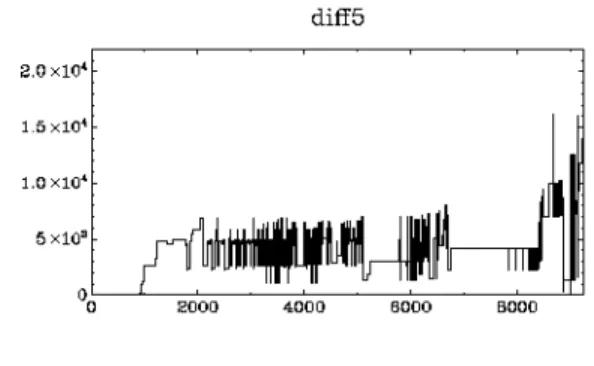
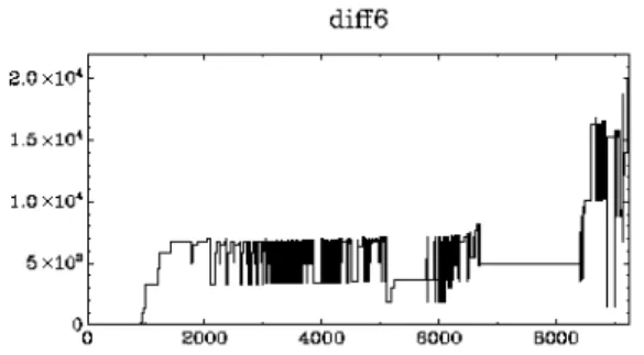
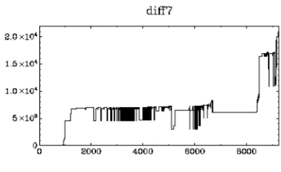
Of course, it is hard to show animations in a paper (all an-imations can be found on the web page). However, because the MSG animation is monotonic, an impression for the an-imation can be obtained using a grey scale approxan-imation. In essence, older stills appear in lighter grey in the approx-imation. (As if they were shown in order, but were slow to fade from the viewing window.) This approximation would not work for a non-monotonic animation as the new images would overlap the older in ways that would make the view useless. For six of the programs shown in Table 1, the grey scale animation approximations are shown in Figure 2.
To give an attempt at a ‘moving image impression’ of the animation in this paper, the animation of the programdiff (Line 8 of Table 1) can be seen as a“flick-book”animation on the upper right corners of this paper.
4.3
Some Interesting Animation Features
This section briefly illustrates the way in which the ani-mation of static analysis can shed light on properties of the static analysis that can be seen in animations much more clearly than in static visualization form. As an example con-sider the animation of the programdiff, which is shown in ‘flick-book’ animation throughout the paper. This anima-tion reveals the movement of a plateau on the right side of the animation. The plateau exists in every still and it rises upward askincreases.
The plateau runs from approximately slice number 7000 through to slice number 8200. Closer examination reveled that this plateau is actually made of several almost identical plateaus. Visual queues exist for this in the middle of the animation (stills diff4 and diff5) in the vertical lines that drop down from the plateau before ‘catching up’.
Each of these separate plateaus comes from a function whose slices include the same statements. The largest is
from the functionregex compile, which compiles regular expression patterns. Just under two thirds of the slices are taken with respect to statements fromregex compile. Any set of statements from a single procedure, such as the ones fromregex compile, that have the same slices whenkis zero, will, by construction, have the same size slice ask increases. Thus, in the animation there is a flat plateau that “rises” during the animation.
In this way, it can be seen that the movement of the plateau corresponds to the presence of a large intraproce-dural connected component. This is not just a dependence cluster (which can be viewed by static visualization [9]) it is a dependence cluster that is formed by one large knot of code within a single procedure. This corresponds to the way in which the plateau tends to ‘rise as one’ as it moves through the animation. By contrast, other dependence clus-ters form gradually as the animation proceeds.
The animation also reveals the formation of a long plateau, running from slices 1000 to 4000 as animation pro-ceeds. Because the animation is not sharp, it is not possi-ble to visually see that this plateau is in fact a plateau from 1000 to 2000 and then a very gradual rise over the next 2000 slices (slice 4000 is less than 1% larger than slice 2000). Although different, these slices share over 99% of the same code, and thus this loss of sharpness has potential advan-tages.
Focusing in on the first 1000 slices of the plateau, the an-imation shows the merging of a collection of sub-plateaus. Looking at the source code, these slices come from 38 func-tions, four of which account for just under two-thirds of the slices. The call sub-graph for these functions contains one self recursive and one pair of mutually recursive functions. Thus as k increases, sub-plateaus should merge together. The animation shows this formation and thus suggests the overall structure of the code. The four plateaus have fully formed indiff5and begin merging in the later stills (e.g., in diff6the latter two have merged).
The animation reveals how large dependence clusters de-pend on intra- and interprocedural dede-pendence clusters. It clarifies that the connection between the various parts of a program can only be observed based on the interprocedural behavior along multiple levels of call depth.
Figure 2. Gray scale approximations for six MSG animations.
5
Related Work
Software Visualization [39, 16] has a long history. How-ever most visualizations are static (e.g., Ball and Eick [7] describe different approaches to visualize static and dy-namic software structures). This can also be referred to as program visualization. The value of dynamic visualization (i.e., animation) is mostly seen in algorithm visualization or algorithm animation, who’s goal is to explain the mecha-nisms that underpin the algorithms concerned. For example, Brown’s work describes a toolbox to support programmers in the construction of hand crafted animations [14]. An-imations are also often used in (visual) debugging, where the state of the debugged program is animated to visualize the change from statement to statement. A recent example is DDD [44]. To the authors’ knowledge, animations have rarely been used to visualize theresults of static program analysis – in contrast to their more common use in, for ex-ample, algorithm animation which would visualize the al-gorithms’ execution. Such approaches often visualize and animate graphs (e.g., the GEVOL system that visualizes the graphical evolution of software, which also uses a flip-book animation [15]).
Unlike the work reported in the present paper, the over-whelming majority of previous work on visualisation has concerned isolated still images, not animation. However, there has been previous work on virtual reality environ-ments [26, 25]. In such work, the virtual environment is animatory. Unlike the work presented in the present pa-per, however, this previous work is immersive (following the principle of immersion in virtual reality). The animation users, is immersed in a virtual world in which objects serve as metaphors for source code constructions. Therefore, the animation exists as a result of the need for movement of the viewers’ point of reference; it does not represent change properties of the source code.
There has also been previous work on properties of vi-sualisations (for example [34]), with similar goals as that set out in Section 2 of the present paper. However, this previous work has tended to focus almost exclusively on non-animatory visualization, and no previous work has con-cerned properties of animations of static source code analy-sis.
Binkley and Harman used slicing to visualize depen-dence clusters [9]. They introduced the MSG, used in the animations reported upon here; the MSG of Binkley and Harman corresponds to the final still in each of the anima-tions described in the present paper.
The present paper used dependence visualisation and slicing as a focus for the case study in animation of static dependence. Current approaches to slicing technology visu-alize results directly in the source code. Some approaches use navigational aids or restricted forms of slicing to im-prove the visualization [3, 17, 40]. Visualizations of slices can be distinguished in graphical and textual visualizations. The SeeSlice slicing tool [6] visualize slices not through source code but with an abstraction representing characters as single pixels.
Other approaches to visualisation of dependence visual-ize the underlying dependence graph [8, 4, 20, 37, 30], how-ever, most authors report that such visualizations become unmanageably large as the size of the systems visualized increases. One advantage of the animation approach intro-duced in the present paper is the way in which scalability is achieved naturally and only at the expense of property of sharpness.
The animation used in the case study in the present pa-per was based on the concept of calling context. The effects on calling context on slicing has been previously studied (but without animation). Some studies examine the trade-off between precision and speed for context-sensitives vs. -insensitive slicing [5, 1, 33, 28, 11]. Krinke [31] has stud-ied the effects of restricting the calling context to a specific call stack.
6
Conclusion and Future Work
This paper has introduced an approach to the animation of static source code analysis that exploits the unavoidable approximate nature of static analysis. The approximate na-ture of static analysis is used to resolve the apparent con-tradiction at the heart of any attempt to animate (which is inherently dynamic) static analysis (which is inherently static).
The paper introduced a framework for defining ap-proaches to animation of static analysis, based upon stills that correspond to levels of approximation available to the analysis. The paper also presented a case study in the ap-plication of this framework to dependence analysis. Results were reported from the implementation of this approach and its application to 13 C programs. The results indicate that the animation is not only interesting but also that it illumi-nates several properties of the dependence structure of the programs that would be hard to visualize without tion. Future work will consider the application the anima-tion framework to other forms of static analysis, such as pointer analysis and context sensitivity.
7
Acknowledgements
The authors wish to thank GrammaTech Inc. for provid-ing CodeSurfer, Dave Binkley is supported by National Sci-ence Foundation grant CCR0305330 (Amorphous Program Slicing). Mark Harman is supported, in part, by EPSRC Grants GR/S93684 (ASTRENET), and GR/T22872 (CON-TRACTS). Binkley and Harman are also supported, in part, by a research grant from DaimlerChrysler, Berlin.
References
[1] G. Agrawal and L. Guo. Evaluating explicitly context-sensitive program slicing. InWorkshop on Program Analysis for Software Tools and Engineering, pages 6–12, 2001. [2] A. V. Aho, R. Sethi, and J. D. Ullman.Compilers: Principles,
techniques and tools. Addison Wesley, 1986.
[3] P. Anderson and T. Teitelbaum. Software inspection using codesurfer. InWorkshop on Inspection in Software Engineer-ing (CAV 2001), 2001.
[4] G. Antoniol, R. Fiutem, G. Lutteri, P. Tonella, S. Zanfei, and E. Merlo. Program understanding and maintenance with the CANTO environment. InInternational Conference on Soft-ware Maintenance, pages 72–81, 1997.
[5] D. C. Atkinson and W. G. Griswold. The design of whole-program analysis tools. InProceedings of the 18th Inter-national Conference on Software Engineering, pages 16–27, 1996.
[6] T. Ball and S. G. Eick. Visualizing program slices. InIEEE Symposium on Visual Languages, pages 288–295, 1994. [7] T. Ball and S. G. Eick. Software visualization in the large.
IEEE Computer, 29(4):33–43, 1996.
[8] F. Balmas. Displaying dependence graphs: a hierarchical ap-proach. InProc. Eigth Working Conference on Reverse Engi-neering, pages 261–270, 2001.
[9] D. Binkley and M. Harman. Locating dependence clus-ters and dependence pollution. In21st IEEE International Conference on Software Maintenance, pages 177–186. IEEE Computer Society Press, 2005.
[10] D. W. Binkley. Interprocedural constant propagation using dependence graphs and a data-flow model. In P. Fritzson, editor,Proceedings of the International Conference on Com-piler Construction, (Edinburgh, Scotland), pages 374–388. Lecture Notes in Computer Science, Volume 786, Springer Verlag, April 1994.
[11] D. W. Binkley and M. Harman. A large-scale empirical study of forward and backward static slice size and context sensi-tivity. InIEEE International Conference on Software Main-tenance, pages 44–53. IEEE Computer Society Press, Sept. 2003.
[12] D. W. Binkley and M. Harman. Analysis and visualization of predicate dependence on formal parameters and global variables. IEEE Transactions on Software Engineering, 30(11):715–735, 2004.
[13] D. W. Binkley and M. Harman. A survey of empirical results on program slicing. Advances in Computers, 62:105–178, 2004.
[14] M. Brown.Algorithm Animation. MIT Press, 1988. [15] C. S. Collberg, S. G. Kobourov, J. Nagra, J. Pitts, and
K. Wampler. A system for graph-based visualization of the evolution of software. InProceedings of the 2003 ACM sym-posium on Software visualization, pages 77–86, 212–213, 2003.
[16] S. Diehl, editor. Software Visualizations, volume 2269 of
LNCS. Springer, 2002.
[17] M. D. Ernst. Practical fine-grained static slicing of optimized code. Technical Report MSR-TR-94-14, Microsoft Research, Redmond, WA, July 1994.
[18] M. D. Ernst, J. Cockrell, W. G. Griswold, and D. Notkin. Dynamically discovering likely program invariants to sup-port program evolution.IEEE Transactions on Software En-gineering, 27(2):1–25, Feb. 2001.
[19] J. Ferrante, K. J. Ottenstein, and J. D. Warren. The program dependence graph and its use in optimization. ACM Trans-actions on Programming Languages and Systems, 9(3):319– 349, July 1987.
[20] K. Gallagher and L. O’Brien. Reducing visualization com-plexity using decomposition slices. InSoftware Visualization Workshop, pages 113–118, 1997.
[21] M. S. Hecht.Flow Analysis of Computer Programs. Elsevier, 1977.
[22] M. Hind. Pointer analysis — haven’t we solved this problem yet? InProgram Analysis for Software Tools and Engineer-ing (PASTE’01). ACM, June 2001.
[23] S. Horwitz, T. Reps, and D. W. Binkley. Interprocedural slicing using dependence graphs.ACM Transactions on Pro-gramming Languages and Systems, 12(1):26–61, 1990. [24] D. Jackson and E. J. Rollins. Chopping: A generalisation of
slicing. Technical Report CMU-CS-94-169, School of Com-puter Science, Carnegie Mellon University, Pittsburgh, PA, July 1994.
[25] C. Knight and M. Munro. Comprehension with[in] virtual environment visualisations. In7thIEEE International Work-shop on Program Comprenhesion (IWPC’99), pages 4–11. IEEE Computer Society Press, May 1999.
[26] C. Knight and M. Munro. Virtual but visible software. In
Information Visualisation, pages 198–205. IEEE Computer Society Press, July 2000.
[27] B. Korel, M. Harman, S. Chung, P. Apirukvorapinit, and R. Gupta. Data dependence based testability transformation in automated test generation. In16thInternational Sympo-sium on Software Reliability Engineering (ISSRE 05), Nov. 2005. To appear.
[28] J. Krinke. Evaluating context-sensitive slicing and chopping. InIEEE International Conference on Software Maintenance, pages 22–31. IEEE Computer Society Press, Oct. 2002. [29] J. Krinke. Advanced Slicing of Sequential and Concurrent
Programs. PhD thesis, Universit¨at Passau, Apr. 2003. [30] J. Krinke. Visualization of program dependence and slices.
InProc. International Conference on Software Maintenance, pages 168–177, 2004.
[31] J. Krinke. Effects of context on program slicing. Journal of Systems and Software, 2006. to appear.
[32] W. Landi and B. G. Ryder. Pointer-induced aliasing: A prob-lem classification. InIn Conference Record of the Eighteenth Annual ACM Symposium on Principles of Programming Lan-guages, pages 93–103. ACM Press, Jan. 1991.
[33] M. Mock, D. C. Atkinson, C. Chambers, and S. J. Eg-gers. Improving program slicing with dynamic points-to data. InProceedings of the 10th International Symposium on the Foundations of Software Engineering, 2002.
[34] M. Pacione, M. Roper, and M. Wood. A comparative evalua-tion of dynamic visualizaevalua-tion tools. InProceedings of WCRE ’03, pages 80–89. IEEE Computer Society, Nov. 2003. [35] T. Reps. Program analysis via graph reachability.
Informa-tion and Software Technology, 40(11–12):701–726, 1998. [36] T. Reps, S. Horwitz, M. Sagiv, and G. Rosay. Speeding up
slicing. InProceedings of the ACM SIGSOFT ’94 Symposium on the Foundations of Software Engineering, pages 11–20, 1994.
[37] D. J. Richardson, T. O. O’Malley, C. T. Moore, and S. L. Aha. Developing and integrating prodag into the arcadia en-vironment. InProceedings of the Fifth Symposium on Soft-ware Development Environments, pages 109–119, 1992. [38] B. G. Ryder, W. Landi, B. Philip, A. Stocks, S. Zhang, and
R. Altucher. A schema for interprocedural modification side-effect analysis with pointer aliasing.ACM Trans. Prog. Lang. Syst., 23(2):105–186, Mar. 2001.
[39] J. T. Stasko, M. H. Brown, and B. A. Price, editors.Software Visualization. MIT Press, Cambridge, MA, USA, 1997. [40] C. Steindl. Benefits of a data flow-aware programming
en-vironment. InWorkshop on Program Analysis for Software Tools and Engineering (PASTE’99), 1999.
[41] P. Tonella, G. Antoniol, R. Fiutem, and E. Merlo. Flow in-sensitive C++ pointers and polymorphism analysis and its ap-plication to slicing. InProceedings of the 19th International Conference on Software Engineering (ICSE ’97), pages 433– 444. IEEE Computer Society Press, May 1997.
[42] M. Weiser. Program slicing.IEEE Transactions on Software Engineering, 10(4):352–357, 1984.
[43] J. Yur, B. G. Ryder, and W. A. Landi. An incremental flow-and context-sensitive pointer aliasing analysis. In Proceed-ings of the 21st International Conference on Software Engi-neering, pages 442–452. IEEE Computer Society Press, May 1999.
[44] A. Zeller. Animating data structures in ddd. InFirst In-ternational Program Visualization Workshop, pages 69–79. University of Joensuu Press, 2001.