University of South Florida
Scholar Commons
Graduate Theses and Dissertations Graduate SchoolNovember 2017
Graph-based Latent Embedding, Annotation and
Representation Learning in Neural Networks for
Semi-supervised and Unsupervised Settings
Ismail Ozsel Kilinc
University of South Florida, [email protected]
Follow this and additional works at:https://scholarcommons.usf.edu/etd
Part of theArtificial Intelligence and Robotics Commons, and theElectrical and Computer Engineering Commons
This Dissertation is brought to you for free and open access by the Graduate School at Scholar Commons. It has been accepted for inclusion in Graduate Theses and Dissertations by an authorized administrator of Scholar Commons. For more information, please contact
Scholar Commons Citation
Kilinc, Ismail Ozsel, "Graph-based Latent Embedding, Annotation and Representation Learning in Neural Networks for Semi-supervised and UnSemi-supervised Settings" (2017).Graduate Theses and Dissertations.
Graph-based Latent Embedding, Annotation and Representation Learning in Neural Networks for Semi-supervised and Unsupervised Settings
by
Ismail Ozsel Kilinc
A dissertation submitted in partial fulfillment of the requirements for the degree of
Doctor of Philosophy
Department of Electrical Engineering College of Engineering
University of South Florida
Major Professor: Ismail Uysal, Ph.D. Sanjukta Bhanja, Ph.D. Selcuk Kose, Ph.D. Lawrence Hall, Ph.D. Umut Ozertem, Ph.D. Date of Approval: November 30, 2017
Keywords: Machine Learning, Deep Learning, Graph-based Regularization, Clustering, Auto-clustering Output Layer
DEDICATION
ACKNOWLEDGMENTS
I would like to express my deepest gratitude to my major professor Dr. Ismail Uysal for his guidance and support in my study. His inspiring suggestions and meticulous feedback in every step of this dissertation enabled me to write it and made it an invaluable experience for me. It has been a pleasure to write this dissertation under his guidance.
I would also wish to express my sincere gratitude to my dissertation committee members Dr. Sanjukta Bhanja, Dr. Selcuk Kose, Dr. Larry Hall and Dr. Umut Ozertem as they kindly accepted to share their invaluable comments and helpful suggestions with me. I also thank to Dr. Kyle Reed as he kindly accepted to chair my dissertation defense meeting.
I express my dearest thanks to Sule Akdogan who did not leave me alone getting through the hardest times. Her presence and her belief in me have been reassuring throughout this study. I am deeply indebted to her for her understanding, patience, respect in what I am doing and encouragement.
Last but not least, most special thanks and love go to my family, Nevin and Tacettin, who have supported me in everything I have done in my life. It could have been impossible to write this dissertation without their love and support. They are the true possessors of my success.
TABLE OF CONTENTS
LIST OF TABLES iii
LIST OF FIGURES v
ABSTRACT vii
CHAPTER 1: INTRODUCTION 1
1.1 Dissertation Outline 5
1.1.1 GAR: An Efficient and Scalable Graph-based Activity
Regu-larization for Semi-supervised Learning 5
1.1.2 Auto-clustering Output Layer: Automatic Learning of Latent
Annotations in Neural Networks 5
1.1.3 Learning Latent Representations in Neural Networks for Unsupervised Clustering through Pseudo Supervision and
Graph-based Activity Regularization 6
CHAPTER 2: GAR: AN EFFICIENT AND SCALABLE GRAPH-BASED AC-TIVITY REGULARIZATION FOR SEMI-SUPERVISED
LEARN-ING 8
2.1 Related Work 10
2.2 Proposed Framework 12
2.2.1 Bipartite Graph Approach 12
2.2.2 Adaptive Adjacency 14
2.2.3 The Optimality of B 15
2.2.4 Activity Regularization 16
2.2.5 Training 18
2.3 Experiments 19
2.3.1 Datasets Used in the Experiments 20
2.3.2 Models Used in the Experiments 20
2.3.3 Results 22
2.3.3.1 MNIST 23
2.3.3.2 SVHN and NORB 26
CHAPTER 3: AUTO-CLUSTERING OUTPUT LAYER: AUTOMATIC
LEARN-ING OF LATENT ANNOTATIONS IN NEURAL NETWORKS 32
3.1 Related Work 35
3.2 Auto-clustering Output Layer 36
3.2.1 Output Layer Modification 36
3.2.2 Mathematical Description and GAR Integration 38
3.2.3 Training and Annotation Assignment 40
3.2.4 Graph Interpretation of the Proposed Framework 40
3.3 Experimental Results 42
3.3.1 MNIST 45
3.3.2 MNIST - Impact of the Provided Supervision on Performance 47
3.3.3 SVHN and CIFAR-100 51
CHAPTER 4: LEARNING LATENT REPRESENTATIONS IN NEURAL NET-WORKS FOR UNSUPERVISED CLUSTERING THROUGH PSEUDO SUPERVISION AND GRAPH-BASED ACTIVITY
REGULAR-IZATION 55
4.1 Background 58
4.2 Proposed Framework 60
4.2.1 Objective Function 60
4.2.2 Modified Affinity and Balance Terms 61
4.2.3 Training and Cluster Assignments 63
4.3 Experiments 63
4.3.1 Experimental Setup and Datasets 63
4.3.2 Quantitative Comparison 66
4.3.3 Representation Properties 68
4.3.4 Graph Interpretation of the Latent Information Propagation
through GAR 70
4.3.5 The Impact of the Number of Clusters k 72
4.3.6 The Impact of Transformations 73
CHAPTER 5: CONCLUSIONS 78
LIST OF TABLES
Table 2.1 Datasets used in the experiments. 21
Table 2.2 Specifications of the models used in the experiments†. 22
Table 2.3 Benchmark results of the semi-supervised test accuracies on MNIST
for few labeled samples, mL∈ {100,600,1000,3000}. 27 Table 2.4 Benchmark results of the semi-supervised test accuracies on SVHN and
NORB. 28
Table 3.1 Datasets used in the experiments. 43
Table 3.2 Specifications of the CNN model used in the experiments†. 44
Table 3.3 Benchmark results for the two-parent case (whether a digit is smaller
or larger than 5) on MNIST. 47
Table 3.4 Benchmark results for the two-parent case on MNIST to observe the
inter-parent effect of the provided supervision. 51
Table 3.5 Test errors for worst, median and best cases among 74 non-repeating
two-parent supervision scenarios on MNIST. 52
Table 3.6 Benchmark error results for the two-parent case on SVHN. 53 Table 3.7 Benchmark error results for the twenty-parent case on CIFAR-100. 54
Table 4.1 Datasets used in the experiments. 64
Table 4.2 Specifications of the CNN model used in the experiments†. 66
Table 4.3 Quantitative unsupervised clustering performance (ACC) on MNIST,
Table 4.4 Quantitative unsupervised clustering performance (NMI) on MNIST,
LIST OF FIGURES
Figure 2.1 MNIST Dataset. 21
Figure 2.2 SVHN Dataset. 22
Figure 2.3 NORB Dataset. 23
Figure 2.4 Visualizations of the graphs G∗, GM andGN for a randomly chosen 250
test examples from MNIST for the mL = 100 case. 24
Figure 2.5 t-SNE visualization of the embedding spaces inferred by B for a
randomly chosen 2000 test examples for themL= 100 case. 26 Figure 2.6 Test accuracies obtained using different models with respect to
unsu-pervised training epochs. 29
Figure 2.7 The effect of bL/bU ratio for MNIST and SVHN datasets. 30 Figure 2.8 The effects of a) on the left, choosing bL ≈ mL and b) on the right,
applying dropout during the unsupervised training on MNIST dataset. 31 Figure 2.9 The effects of a) cα/c
β and b)cF on MNIST dataset. 31
Figure 3.1 Particular semi-supervised setting discussed in this chapter. 34
Figure 3.2 Neural network structure with the ACOL. 37
Figure 3.3 After training, the pooling layer is simply disconnected. 41
Figure 3.4 CIFAR-100 Dataset. 43
Figure 3.5 Visualizations of the graph GY and its spanning subgraph GM for a
randomly chosen 250 test examples from MNIST. 46
Figure 3.6 t-SNE visualization of the latent space inferred by Z for a randomly
Figure 3.7 t-SNE visualization of the latent spaces obtained using four different
approaches for a randomly chosen 2000 test examples from MNIST. 49 Figure 3.8 t-SNE visualization of the latent spaces obtained for the first
parent-class, {0,1,2,3,4}, showing the inter-parent effect of the provided
supervision. 50
Figure 3.9 Normalized histogram of the test accuracies obtained using ACOL for a randomly chosen 74 non-repeating two-parent supervision scenarios
on MNIST. 52
Figure 4.1 Assume that we are given a dataset of hand-written digits such as MNIST where the overall task is the complete categorization of each
digit. 59
Figure 4.2 USPS Dataset. 65
Figure 4.3 t-SNE visualization of the latent space F throughout the training for
a randomly selected 2000 untransformed test examples from MNIST. 67 Figure 4.4 The average value for each dimension ofF,Zandsoftmax(Z)observed
with respect to untransformed test set examples and the norm of the
associated weights. 71
Figure 4.5 Comparison of t-SNE visualizations of the latent spaces F, Z and
softmax(Z) for 2000 test examples from MNIST. 72
Figure 4.6 Visualizations of the graph GY and its spanning subgraph GM for
randomly chosen 250 test examples from MNIST. 75
Figure 4.7 Illustration of a few examples of each cluster for two differentk settings. 76 Figure 4.8 t-SNE visualizations of the representation spaces observed when
ABSTRACT
Machine learning has been immensely successful in supervised learning with out-standing examples in major industrial applications such as voice and image recognition. Following these developments, the most recent research has now begun to focus primarily on algorithms which can exploit very large sets of unlabeled examples to reduce the amount of manually labeled data required for existing models to perform well. In this dissertation, we propose graph-based latent embedding/annotation/representation learning techniques in neural networks tailored for semi-supervised and unsupervised learning problems. Specifically, we propose a novel regularization technique called Graph-based Activity Regularization (GAR) and a novel output layer modification called Auto-clustering Output Layer (ACOL) which can be used separately or collaboratively to develop scalable and efficient learning frameworks for semi-supervised and unsupervised settings.
First, singularly using the GAR technique, we develop a framework providing an effective and scalable graph-based solution for semi-supervised settings in which there exists a large number of observations but a small subset with ground-truth labels. The proposed approach is natural for the classification framework on neural networks as it requires no additional task calculating the reconstruction error (as in autoencoder based methods) or implementing zero-sum game mechanism (as in adversarial training based methods). We demonstrate that GAR effectively and accurately propagates the available labels to unlabeled examples. Our results show comparable performance with state-of-the-art generative approaches for this setting using an easier-to-train framework.
Second, we explore a different type of semi-supervised setting where a coarse level of labeling is available for all the observations but the model has to learn a fine, deeper level of latent annotations for each one. Problems in this setting are likely to be encountered in many domains such as text categorization, protein function prediction, image classification as well as in exploratory scientific studies such as medical and genomics research. We consider this setting as simultaneously performed supervised classification (per the available coarse labels) and unsupervised clustering (within each one of the coarse labels) and propose a novel framework combining GAR with ACOL, which enables the network to perform concurrent classification and clustering. We demonstrate how the coarse label supervision impacts performance and the classification task actually helps propagate useful clustering information between sub-classes. Comparative tests on the most popular image datasets rigorously demonstrate the effectiveness and competitiveness of the proposed approach.
The third and final setup builds on the prior framework to unlock fully unsupervised learning where we propose to substitute real, yet unavailable, parent- class information with pseudo class labels. In this novel unsupervised clustering approach the network can exploit hidden information indirectly introduced through a pseudo classification objective. We train an ACOL network through this pseudo supervision together with unsupervised objective based on GAR and ultimately obtain a k-means friendly latent representation. Furthermore, we demonstrate how the chosen transformation type impacts performance and helps propagate the latent information that is useful in revealing unknown clusters. Our results show state-of-the-art performance for unsupervised clustering tasks on MNIST, SVHN and USPS datasets with the highest accuracies reported to date in the literature.
CHAPTER 1: INTRODUCTION
Artificial intelligence (AI) is a flourishing field with many practical applications and active research topics such as automating routine work, understanding and interpreting speech, text and images, supporting basic scientific research and diagnosis in medicine [19]. In the early days of AI dominant approaches were rule-based systems where the knowledge needed to solve the tasks is explicitly hard-coded by a programmer. These kinds of approaches have been successful in solving problems that can be easily described by a small set of formal rules but can require a lot of search, such as playing chess; however, they failed to solve those that cannot be formally described, such as recognizing objects or speech, and those requiring an immense amount of knowledge, such as playing Go. While there are approximately 400 possible next moves in chess, for Go this number goes up to 130,000 [13]. Also, it is impossible for a programmer to hard-code the knowledge required to recognize faces through if-else based rules. Therefore, researchers have reached a consensus that, in order to behave in an intelligent way, AI systems need the ability to acquire their own knowledge from raw data, which is known as the field of machine learning, just as human-beings learn from experience. Neural networks, when first introduced as universal estimators, created wide spread enthusiasm especially with innovative and bio-inspired machine learning methodologies such as error back-propagation [54]. However, their potential wasn’t fully realized until greater availability of computational power to simulate networks orders of magnitude larger than their early counterparts and massive datasets to help train them. This approach to AI, called deep learning with reference to deep structures with many layers, has been proposed to mimic the operational and organizational behavior of the human brain, which works through
abstraction [3]. For example, objects or sounds are represented as electrical signals traveling through different types of connections with different strengths between neurons in visual or auditory cortexes respectively [46]. Deep learning takes inspiration from this and relies on higher-level representations of features (or characteristics) embedded in the data instead of human engineered characteristics.
One great example is in computer vision in regards to how methods have changed transformatively over the last several years. For instance, a particular implementation of deep learning called Convolutional Neural Networks (CNN) has been applied to the image classification problem with remarkable success [31]. Besides pure performance numbers, the most interesting finding was how expert human engineered features, such as textures and contrasts, which have been used for decades were ultimately represented at the deeper and hidden layers of the neural network without any explicit instructions. On the other hand, for tasks involving temporal input such as speech and text, Recurrent Neural Networks (RNN) are widely in use since they provide better prediction for the future elements thanks to the architecture implicitly keeping the information about past elements, such as Long Short Term Memory (LSTM) networks [34], [23].
Specifically in the last five year period, these models have successful produced many practical industrial applications for supervised learning problems where the overall task is to learn to map one vector (input) to another (label), given enough examples of the mapping. To achieve good performance, algorithms used for these applications require large amounts of labeled data whose labels are typically entered by a staff of human supervisors. However, labeling is mostly a challenging task that sometimes requires expert knowledge and in fact, especially in exploratory research, defines the scientific problem itself. Therefore, in recent years, researchers have focused approaches that are able to exploit a large set of unlabeled examples to reduce the amount of labeled data required for existing models to perform well. These approaches adopt some form of unsupervised or semi-supervised learning. In a
semi-supervised setting, the goal is to take advantage of a large set of unlabeled examples to improve the performance that is obtained using only labeled examples whose amount is typically much smaller than that of unlabeled ones. On the other hand, in an unsupervised setting, as there is no labeling available, the task is generally to determine the underlying distribution generating the dataset and to discover the unknown labels.
In this dissertation, we propose graph-based latent embedding, annotation and represen-tation learning in neural networks for semi-supervised and unsupervised settings. Specifically, we propose a novel regularization technique called Graph-based Activity Regularization (GAR) and a novel output layer modification called Auto-clustering Output Layer (ACOL) which are separately and collaboratively used to develop scalable and efficient learning frameworks for semi-supervised and unsupervised settings. More specifically, major contributions of this dissertation are as follows:
• The first graph-based technique in literature which displays competitive performance with deep generative approaches based on the test performances on mid-size image datasets of digits, such as MNIST [35] and SVHN [44]
– 6.98%(±0.82)1 vs. 4.28% [41] error rate on SVHN using a randomly chosen 1000 labeled examples with stratification
– 1.56%(±0.09)1 vs. 0.93%(±0.07) [56] error rate on MNIST using a randomly chosen 100 labeled examples with stratification
and statistically significantly outperforms all other graph-based methods
– 1.56%(±0.09)1 vs. 7.75%(±0.07) [67] error rate on MNIST using a randomly chosen 100 labeled examples with stratification
for semi-supervised learning. 1±shows the 0.95 confidence interval
• The first model in literature which enables neural networks to learn previously unknown annotations in observations for which coarse labeling is available with empirical demonstrations of how inter-class differences can help explore subclasses of the provided coarse labeling.
• Statistically significant and superior performance with respect to other methods modified to operate in this particular setting based on the test performances on MNIST, i.e. mid-size image dataset of hand-written digits
– 1.39%(±0.12)1 vs. 8.18% [25] error rate on MNIST when providing the coarse labeling as whether a digit is smaller or greater than 5
• The first graph-based technique in literature which outperforms all other known approaches for unsupervised clustering based on the test performances on mid-size image datasets of digits, such as MNIST [35] and SVHN [44]
– 76.80%(±1.30)1 vs. 57.30%(±3.90) [24] clustering accuracy on SVHN
– 98.32%(±0.08)1 vs. 98.40%(±0.40) [24] and 96.10 [72] clustering accuracy on MNIST
and defines the current state-of-the-art for unsupervised clustering for the SVHN dataset, as observed through statistically significantly better result with a wide margin.
The following section describes the outline of the dissertation and briefly summarizes the proposed framework in each chapter.
1.1 Dissertation Outline
1.1.1 GAR: An Efficient and Scalable Graph-based Activity Regularization for Semi-supervised Learning
In Chapter 2, we propose a novel graph-based approach for the semi-supervised learning setting in which there exist a large number of observations but only a small subset of them have ground-truth labels. In this approach, the adjacency of the examples is inferred using the predictions of a neural network model, which is first initialized by supervised training using the small subset of labeled examples. Then, during the subsequent unsupervised portion of the training that propagates the available labels toward the unlabeled examples, the inferred adjacency matrix is simultaneously updated along with the predictions of the network. However, unlike traditional graph-based methods propagating the labels using an m×m adjacency matrix of m examples, the proposed approach propagates the labels through a scalable regularization objective defined on an n × n adjacency matrix of n output classes, where typically n m. Ultimately, the proposed framework provides an effective and scalable graph-based solution which is natural for the classification framework on neural networks as it requires no additional task calculating the reconstruction error (as in autoencoder based methods) or implementing zero-sum game mechanism (as in adversarial training based methods). Our results show comparable performance with state-of-the-art generative approaches for semi-supervised learning using an easier-to-train framework. 1.1.2 Auto-clustering Output Layer: Automatic Learning of Latent Annotations in
Neural Networks
In Chapter 3, we discuss a different type of semi-supervised setting: a coarse level of labeling is available for all observations but the model has to learn a fine level of latent annotation for each one of them. Problems in this setting are likely to be encountered in many domains such as text categorization, protein function prediction, image classification as
well as in exploratory scientific studies such as medical and genomics research. We consider this setting as simultaneously performed supervised classification (per the available coarse labels) and unsupervised clustering (within each one of the coarse labels) and propose a novel output layer modification called auto-clustering output layer (ACOL) that allows concurrent classification and clustering based on Graph-based Activity Regularization (GAR) technique. As the proposed output layer modification duplicates the softmax nodes at the output layer for each class, GAR allows for competitive learning between these duplicates on a traditional error-correction learning framework to ultimately enable a neural network to learn the latent annotations in this partially supervised setup. We demonstrate how the coarse label supervision impacts performance and helps propagate useful clustering information between sub-classes. Comparative tests on three image datasets MNIST, SVHN and CIFAR-100 rigorously demonstrate the effectiveness and competitiveness of the proposed approach. 1.1.3 Learning Latent Representations in Neural Networks for Unsupervised
Cluster-ing through Pseudo Supervision and Graph-based Activity Regularization
In Chapter 4, we propose a novel unsupervised clustering approach exploiting the hidden information that is indirectly introduced through a pseudo classification objective. Specifically, we randomly assign a pseudo parent-class label to each observation which is then modified by applying the domain specific transformation associated with the assigned label. Generated pseudo observation-label pairs are subsequently used to train a neural network with Auto-clustering Output Layer (ACOL) that introduces multiple softmax nodes for each pseudo parent-class. Due to the unsupervised objective based on Graph-based Activity Regularization (GAR) terms, softmax duplicates of each parent-class are specialized as the hidden information captured through the help of domain specific transformations is propagated during training. Ultimately we obtain a k-means friendly latent representation. Furthermore, we demonstrate how the chosen transformation type impacts performance and
helps propagate the latent information that is useful in revealing unknown clusters. Our results show state-of-the-art performance for unsupervised clustering tasks on MNIST, SVHN and USPS datasets, with the highest accuracies reported to date in the literature.
CHAPTER 2: GAR: AN EFFICIENT AND SCALABLE GRAPH-BASED ACTIVITY REGULARIZATION FOR SEMI-SUPERVISED LEARNING1
The idea of utilizing an auxiliary unsupervised task to help supervised learning dates back to 90s [59]. As an example to one of its numerous achievements, unsupervised pretraining followed by supervised fine-tuning was the first method to succeed in the training of fully connected architectures [22]. Although today it is known that unsupervised pretraining is not a must for successful training, this particular accomplishment played an important role enabling the current deep learning renaissance and has become a canonical example of how a learning representation for one task can be useful for another one [19]. There exist a variety of approaches to combine supervised and unsupervised learning in the literature. More specifically, the term semi-supervised is commonly used to describe a particular type of learning for applications in which there exists a large number of observations, where a small subset of them has ground-truth labels. Proposed approaches aim to leverage the unlabeled data to improve the generalization of the learned model and ultimately obtain a better classification performance.
One approach is to introduce additional penalization into training based on the reconstruction of the input through autoencoders [50]. Recently, there have been significant improvements in this field following the introduction of a different generative modeling technique which uses the variational equivalent of deep autoencoders integrating stochastic latent variables into the conventional architecture [29] [53]. First, [28] have shown that such modifications make generative approaches highly competitive for semi-supervised learning.
1This chapter has been submitted to peer-reviewed Elsevier Neurocomputing Journal and is now under
Later, [37] further improved the results obtained using variational autoencoders by introducing auxiliary variables increasing the flexibility of the model. Furthermore, [52] has applied Ladder networks [61], a layer-wise denoising autoencoder with skip connections from the encoder to the decoder, for semi-supervised classification tasks.
On the other hand, these recent improvements have also motivated researchers to offer radically novel solutions such as virtual adversarial training [42] motivated by Generative Adversarial Nets [20] proposing a new framework corresponding to a minimax two-player game. Alternatively, [73] revisited graph-based methods with new perspectives such as invoking the embeddings to predict the context in the graph. Conventional graph-based methods aim to construct a graph propagating the label information from labeled to unlabeled observations and connecting similar ones using a graph Laplacian regularization in which the key assumption is that nearby nodes are likely to have the same labels [74], [7]. However, the requirement for eigenanalysis of the graph Laplacian severely limits the scalability of these approaches. In a different work, [67] have shown that the idea of combining an embedding-based regularizer with a supervised learner to perform semi-supervised learning can be generalized to deep neural networks and the resulting models can be trained by stochastic gradient descent. A possible bottleneck with this approach is that the optimization of the unsupervised part of the loss function requires precomputation of the weight matrix specifying the similarity or dissimilarity between the examples whose size grows quadratically with the number of examples. For example, a common approach to computing the similarity matrix is to use the k-nearest neighbor algorithm which is computationally very expensive for a large number of samples. Therefore, it is approximated using sampling techniques.
In this chapter, we propose a novel framework for semi-supervised learning which can be considered a variant of graph-based approach. This framework can be described as follows.
• Instead of a graph between examples, we consider a bipartite graph between examples and output classes. To define this graph, we use the predictions of a neural network
model initialized by a supervised training process that uses a small subset of samples with known labels.
• We use this bipartite graph to obtain two disjoint graphs, which are then employed to interpret two adjacencies: One between the examples and another between the output nodes. We introduce two regularization terms for the graph between the output nodes and during the unsupervised portion of training, the predictions of the network are updated only based on these two regularizers.
• These terms implicitly provide that the bipartite graph between the examples and the output classes becomes a biregular graph and the inferred graph between the examples becomes a disconnected graph of regular subgraphs. Ultimately, because of this observation, the predictions of the network yield embeddings that we try to find. The proposed framework is naturally inductive, where predictions can be generalized to never-seen-before examples. More importantly, it is scalable and it can be applied to datasets regardless of the sample size or the dimensionality of the feature set. Furthermore, the entire framework operationally implements the same feedforward and backpropagation mechanisms of the state of the art deep neural networks as the proposed regularization terms are added to the loss function in the same way as adding standard L1, L2 regularizations [45] and similarly optimized using stochastic gradient descent [12].
2.1 Related Work
Consider a semi-supervised learning problem where out of m observations, correspond-ing ground-truth labels are only known for a subset of mL examples and the labels of the complimentary subset of mU examples are unknown where m = mL +mU and typically mL mU. Let x1:m and y1:m denote the input feature vectors and the output predictions respectively and t1:mL denote the available output labels. The main objective is to train a
classifier f : x→ y using all m observations that is more accurate than another classifier trained using only the labeled examples. Graph-based semi-supervised methods consider a connected graphG = (V,E)of which verticesV correspond to allm examples and edgesE are specified by an m×m adjacency matrix Awhose entries indicate the similarity between the vertices. There have been many different approaches about the estimation of the adjacency matrix A. [74] derived Aaccording to simple Euclidean distances between the samples while [67] precomputed A using ak-nearest neighbor algorithm. They also suggest that, in case of a sequential data, one can presume consecutive instances are also neighbors in the graph. [73], on the other hand, consider the specific case where Ais explicitly given and represents additional information. The most important common factor in all these graph-based methods is the fact thatAis a fixed matrix throughout the training procedure with the key assumption that nearby samples on G, which is defined by A, are likely to have the same labels. Hence, the generic form of the loss function for these approaches can be written as:
mL X i=1 L f(xi), ti +λ m X i,j=1 U f(xi), f(xj), Aij (2.1)
where L(.) is the supervised loss function such as log loss, hinge loss or squared loss,U(.)is the unsupervised regularization (in which a multi-dimensional embedding g(xi) =zi can also be replaced with one-dimensional f(xi)) andλ is a weighting coefficient between supervised and unsupervised metrics of the training L(.) and U(.). One of the commonly employed embedding algorithms in semi-supervised learning is Laplacian Eigenmaps [6] which describes the distance between the samples in terms of the Laplacian L= D−A, where D is the diagonal degree matrix such that Dii =
P
jAij. Then, unsupervised regularization becomes: m X i,j=1 U g(xi), g(xj), Aij = m X i,j=1 Aij||g(xi)−g(xj)||2 = Tr(ZTLZ) (2.2)
subject to the balancing constraint ZTDZ = I, where Z = [z1, ...,zm]T. [74] used this regularization together with a nearest neighbor classifier while [7] integrates hinge loss to train an SVM. Both methods impose regularization on labels f(xi). On the other hand, [67] employ a margin-based regularization by [21] such that
U f(xi), f(xj), Aij = ||f(xi)−f(xj)||2 if Aij = 1 max(0, γ− ||f(xi)−f(xj)||2) if Aij = 0 (2.3)
to eliminate the balancing constraints and enable optimization using gradient descent. They also propose to learn multi-dimensional embeddings on neural networks such that g(xi) = fl(x
i) =yli, whereyli is the output of the lth hidden layer corresponding to the ith sample.
2.2 Proposed Framework
2.2.1 Bipartite Graph Approach
Instead of estimating the adjacency matrix Ausing an auxiliary algorithm such as nearest neighbor or auxiliary external knowledge, we propose to use the actual predictions of a neural network model initialized by a supervised training step using mL labeled examples.
Suppose that after supervised training, predictions of the network, B, for all m examples are obtained as anm×n matrix, where n is the number of output classes and Bij is the probability of the ith example belonging to jth class. We observe that these predictions, indeed, define a bipartite graph G∗ = (V∗,E∗) whose vertices V∗ are m examples together
with n output nodes. However, V∗ can be divided into two disjoint sets M and N, such
that G∗ = (M,N,E∗), where Mis the set of examples,N is the set of output nodes and an
edge e∈ E∗ connects an example m∈ M with an output noden∈ N. As there is no lateral
matrix A∗ of graphG∗ has the following form A∗ = 0m×m Bm×n BTn×m 0n×n (2.4)
where B corresponds to m×n biadjacency matrix of graph G∗ which is by itself unique and
sufficient to describe the entire E∗.
In graphG∗, the examples are connected with each other by even-length walks through
the output nodes whereas the same is true for the output nodes through the samples. In this case, the square of the adjacency matrix A∗ represents the collection of two-walks (walks with two edges) between the vertices. It also implements two disjoint graphs GM= (M,EM)
and GN = (N,EN)such that
A∗2 = BBTm×m 0m×n 0n×m BTBn×n = M 0 0 N (2.5)
where M =BBT and N =BTB are the adjacency matrices specifying edges EM and EN, respectively. Unlike a simple graph G considered by conventional graph-based methods, GM
also involves self-loops. However, they have no effect on the graph Laplacian and thus on the embeddings. Hence, one can estimate the adjacency of examples using the predictions of the network, i.e. M = BBT, and then find the embeddings by applying a standard unsupervised objective such as Laplacian Eigenmap minimizing Tr(ZTLMZ) as defined in (2.2), where LM = DM −M. It is important to note that conventional graph-based algorithms assume a fixed adjacency matrix during loss minimization whereas in the proposed framework, we consider an adaptive adjacency which is updated throughout the unsupervised training process as described in the following section.
2.2.2 Adaptive Adjacency
As derived adjacency M depends only on B, during the unsupervised training, B
needs to be well-constrained to preserve the learned latent embeddings. Otherwise, the idea of updating the adjacency matrix throughout an unsupervised task might be catastrophic and results in offsetting the effects of the supervised training step.
There are two constraints derived from the natural expectation of the specific form of the B matrix for a classification problem: i) first, a sample is to be assigned to one class with the probability of 1, while remaining n−1 classes have 0 association probability, and ii) second, for balanced classification tasks, each class is expected to involve approximately the same number of the examples. Let us first consider the case where B assigns m/n examples to each one of the n classes with the probability of 1. B in this particular form implies that graph G∗ becomes (1,m/n)-biregular since
deg(mi) = 1,∀mi ∈ M and deg(ni) =m/n,∀ni ∈ N (2.6)
Subsequently graph GN turns into a disconnected graph including only self-loops and its adjacency matrix N becomes a scaled identity matrix indicating mutually exclusive and uniform distribution of the examples across the output nodes. Similarly, GM also becomes a disconnected graph includingndisjoint subgraphs. Each one of these subgraphs ism/n-regular, where each vertex also has an additional self-loop. In this particular form, B becomes the optimal embedding of M as it satisfies both BTLMB=0 and BTDMB =I where LM is the Laplacian and DM is the diagonal degree matrix of M (as shown in the Section 2.2.3). As they all depend only on B, the relationships between G∗, GM andGN are biconditional,
which can be written as follows:
G∗ is (1,m/n)-biregular⇔ GM : argmin ZTD
MZ=I
Depending on this relation, we propose applying regularization during the unsupervised task in order to ensure that N becomes the identity matrix. Regularizing N instead ofM
enables us to devise a scalable framework as typically nm. The first one of the proposed two regularization terms constrainsN to be a diagonal matrix, whereas the second one forces it into becoming a scaled identity matrix by equalizing the value of the diagonal entries. The second term ultimately corresponds to constraining B to obtain a uniform distribution of samples across the output classes. Obviously, this condition is not valid for every dataset, but a balancing constraint is required to prevent collapsing onto a subspace of dimension less than n and it is analogous to the constraint of ZTDZ =I in [6].
2.2.3 The Optimality of B
Following [6], the optimal embedding that can be found on M =BBT can be written as
argmin ZTD
MZ=I
Tr(ZTLMZ) (2.8)
where LM is the Laplacian and DM is the diagonal degree matrix of M such that LM = DM −M. For any embedding Z, one can simply write that
ZTLMZ =ZTDMZ −ZTM Z (2.9)
Replacing M with BBT, then (2.9) becomes
ZTLMZ =ZTDMZ−ZTBBTZ (2.10)
If the regularization turnsN =BTB into the identity matrix, using B as the embedding yields that
BTLMB=BTDMB−I (2.12) and this equality is satisfied when BTLMB =0 and BTDMB=I. Then,
argmin ZTD
MZ=I
Tr(ZTLMZ) = B (2.13)
Assuming that the proposed regularization successfully turns N into the identity matrix, this simply tells us that no additional step is necessary to find the optimal embedding of M and
B automatically becomes an optimal embedding. 2.2.4 Activity Regularization
Consider a neural network with L−1 hidden layers where l denotes the individual index for each hidden layer such that l ∈ {1, ..., L−1}. Let Y(l) denote the output of the nodes at layer l. Y(0) =X is the input and f(X) =f(L)(X) =Y(L)=Y is the output of the entire network. W(l) andb(l) are the weights and biases of layer l, respectively. Then, the feedforward operation of the neural networks can be written as
Y(l)=f(l) X=h(l) Y(l−1)W(l)+b(l) (2.14)
where h(l)(.) is the activation function applied at layerl.
In the proposed framework, instead of using the output probabilities of the softmax nodes, we use the activations at their inputs to calculate the regularization. The intuition here is that regularizing linear activations rather than nonlinear probabilities defines an easier optimization task. Since the multiplication of two negative activations yields a positive (false) adjacency inM, we rectify the activations first, i.e. f(x) = max(0, x). Then,B becomes
B=g X = max 0, Y(L−1)W(L)+b(L) (2.15)
Recall that N is an n×n symmetric matrix such that N := BTB and let v be a
1×n vector representing the diagonal entries of N such that v :=
N11 N22 . . . Nnn
. Then, let us define V as an n×n symmetric matrix such that V :=vTv. Then, the two proposed regularization terms can be written as
Affinity=α B := n P i6=j Nij (n−1) n P i=j Nij (2.16) and Balance=β B := n P i6=j Vij (n−1) n P i=j Vij (2.17)
While affinity penalizes the non-zero off-diagonal entries of N, balance attempts to equalize diagonal entries. One might suggest minimizing the off-diagonal entries ofN directly without normalizing, however, normalization is required to bring both regularizers within the same range for optimization and ultimately to ease hyperparameter adjustment. Unlike regularizing N to simply become a diagonal matrix, equalizing the diagonal entries is not an objective that we can reach directly by minimizing some entries of N. Hence, we propose to use (2.17) that takes values between 0 and 1 where 1 represents the case where all diagonal entries of N are equal. Respectively, we propose to minimize the normalized term (2.16) instead of the direct summation of the off-diagonal entries. However, during the optimization, denominators of these terms increase with the activations which may significantly diminish the effects of both regularizers. To prevent this phenomenon, we apply the L2 norm to penalize the increase of the sum of squared activities. Recall that the Frobenius norm for B,
||B||F, is analogous to the L2 norm of a vector and defined as
||B||F =
q X
B2
Hence, the proposed overall unsupervised regularization loss ultimately becomes U g X=U B =cαα B +cβ 1−β B +cF||B||2F (2.19)
and can be written in terms of B as
U B =cα 2 n−1 P i=1 n P j=i+1 m P k=1 BkiBkj (n−1) n P i=1 m P k=1 B2 ki +cβ n−1 P i=1 n P j=i+1 m P k=1 B2 ki− m P k=1 B2 kj 2 (n−1) n P i=1 m P k=1 B4 ki +cF n P i=1 m P k=1 Bki2 (2.20) 2.2.5 Training
Training of the proposed framework consists of two sequential steps: Supervised training using only the labeled examples and subsequent unsupervised regularization using the entire dataset. We adopt stochastic gradient descent in the mini-batch mode [12] for optimization of both steps. Indeed, mini-batch mode is required for the unsupervised task since the proposed regularizers implicitly depend on the comparison of the examples with each other. Algorithm 1 below describes the entire training procedure. The first stage of the training is a typical supervised training task in which mL examples XL= [x1, ...,xmL]
T
are introduced to the network with the corresponding ground-truth labelstL= [t1, ..., tmL] T
and the network parameters are updated to minimize the log loss L(.). After the supervised training step is completed, this supervised objective is never revisited and the labels tL are never reintroduced to the network in any part of the unsupervised task. Hence, the remaining unsupervised objective is driven only by the proposed regularization loss U(.) defined in (2.19). The examplesXL used in the supervised training stage can also be batched together with the upcoming unlabeled examples XU = [xmL+1, ...,xm]
T in order to ensure a more
stable regularization. As the network is already introduced to them, bL examples randomly chosen from XL can be used as guidance samples for the remaining bU examples ofXU in
that batch. Such blended batches help the unsupervised task especially when the examples in the dataset have high variance.
Algorithm 1: Model training Supervised training: Input :XL= [x1, ...,xmL] T,t L= [t1, ..., tmL] T, batch size b repeat
(X´1,´t1), ...,(X´mL/b,´tmL/b) ←−(XL,tL) // Shuffle and create batch
pairs, e.g. if mL= 1000 and b= 100, then 10 pairs vs. 100 for
batch size
fori←1 to mL/b do
Take ith pair (X´i,t´i)
Take a gradient step for L f X´i
,´ti
untilstopping criteria is met returnmodel Unsupervised training: Input :model,XL= [x1, ...,xmL] T,X U = [xmL+1, ...,xm] T,b L,bU repeat ´
X1, ...,X´mU/bU, ←−XU // Shuffle and create input batches
fori←1 to mU/bU do
Take ith input batchX´i
¨
X ←−random(XL, bL) // Randomly sample bL examples from XL
Take a gradient step for U g hX´T
i X¨
TiT
untilstopping criteria is met
2.3 Experiments
The models have been implemented in Python using Keras [14] and Theano [60]. Open source code is available at http://github.com/ozcell/LALNets that can be used to reproduce the experimental results obtained on the three image datasets, MNIST [35], SVHN [44] and NORB [36] have been used by previous researchers [18, 28, 33, 37, 41, 42, 52, 56, 65, 67] publishing in the field of semi-supervised learning at NIPS and other similar venues.
2.3.1 Datasets Used in the Experiments
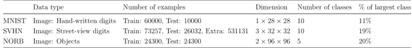
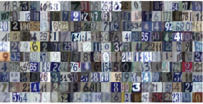
Figures 2.1, 2.2 and 2.3 respectively illustrate 200 examples from MNIST, SVHN and NORB datasets and Table 2.1 summarizes the properties of these datasets used in the experiments. The MNIST is a dataset of handwritten digits in which digits have been size-normalized and centered in a fixed-size image [35]. SVHN is a real-world color image dataset that can be seen as similar in flavor to MNIST, but comes from a significantly harder, real world problem, i.e. recognizing digits and numbers in natural scene images [44]. NORB, on the other hand, is a dataset of grayscale images of 50 toys belonging to 5 generic categories: four-legged animals, human figures, airplanes, trucks, and cars. The objects were imaged by two cameras under 6 lighting conditions, 9 elevations and 18 azimuths. Its training set is composed of 5 instances of each category and test set of the remaining 5 instances [36]. The following preprocessing steps have been applied to these datasets.
• MNIST: Images were normalized by dividing by 256.
• SVHN: We applied centering and normalization per each channel, i.e. we set each sample mean to 0 and divided each input by its standard deviation.
• NORB: Following [37], images were downsampled to 32×32 using nearest-neighbor interpolation. We added uniform noise between 0 and 1 to each pixel value. First, we normalized the NORB dataset by dividing by 256, then applied centering and normalization per each channel and also set input mean to 0 over the dataset and divided inputs by standard deviation of the dataset.
2.3.2 Models Used in the Experiments
Table 2.2 summarizes all models used in the experiments. Reported MNIST results have been obtained using the model named6-layer CNN, whereas SVHN results were obtained
Figure 2.1: MNIST Dataset.
Table 2.1: Datasets used in the experiments.
Data type Number of examples Dimension Number of classes % of largest class
MNIST Image: Hand-written digits Train: 60000, Test: 10000 1×28×28 10 11%
SVHN Image: Street-view digits Train: 73257, Test: 26032, Extra: 531131 3×32×32 10 19%
NORB Image: Objects Train: 24300, Test: 24300 2×96×96 5 20%
using the 9-layer CNN-2 model and NORB results were obtained using the 9-layer CNN model. The results obtained on different models are also presented in the following sections to show the effect of the chosen model on the test accuracy. The ReLU activation function [43], i.e. f(x) = max(0, x), has been used for all models. For both supervised training and unsupervised regularization, models were trained using stochastic gradient descent with following settings: learning rate= 0.01, decay= 1e−6, momentum= 0.95 with Nesterov updates, where the momentum direction is first applied and then this direction is corrected with a gradient update [8].
Figure 2.2: SVHN Dataset.
Table 2.2: Specifications of the models used in the experiments†. Model name Specification
4-layer MLP FC(2048) - Drop(0.5) - FC(2048) - Drop(0.5) - FC(2048) - Drop(0.5) - FC(n)
6-layer CNN 2*Conv(32x3x3) - MP(2x2) - Drop(0.2) - 2*Conv(64x3x3) - MP(2x2) - Drop(0.3) - FC(2048) - Drop(0.5) - FC(n)
9-layer CNN 2*Conv(32x3x3) - MP(2x2) - Drop(0.2) - 2*Conv(64x3x3) - MP(2x2) - Drop(0.3) - 3*Conv(128x3x3) - MP(2x2) - Drop(0.4) - FC(2048) - Drop(0.5) - FC(n) 9-layer CNN-2 2*Conv(64x3x3) - MP(2x2) - Drop(0.2) - 2*Conv(128x3x3) - MP(2x2) - Drop(0.3) - 3*Conv(256x3x3) - MP(2x2) - Drop(0.4) - FC(2048) - Drop(0.5) - FC(n)
†Inputs of the models are determined according to the dimensions of the dataset being used for the training.nis the number of classes. FC(i): Fully connected layer withiunits
Drop(i): Applying dropout[58] where the probability of retaining a unit is1−i
Conv(i×j×k): Convolution layer whereicorresponds to the number of filters andj×kto the kernel size MP(i×j): Max pooling with pool size ofi×j, i.e. factors by which to downscale (vertical×horizontal)
2.3.3 Results
Coefficients of the proposed regularization term have been chosen as cα = 3, cβ = 1 and cF = 0.000001 in all of the experiments. For the sake of fairness, in the same manner as followed by the models used for the comparison [42], a validation set of 1000 examples has been chosen randomly without stratification among the training set examples to determine the hyperparameters of the proposed approach (cα, cβ, cF,bL/bU), the specifications of the models used for the experiments (given in Table 2.2) and the epoch to report the test accuracy. We
Figure 2.3: NORB Dataset.
used a batch size of 128 for both supervised training and unsupervised regularization steps. For each dataset, the same strategy is applied to decide on the ratio of labeled and unlabeled data in the unsupervised regularization batches, i.e. bL/bU: among a hyperparameter set of
{16,32,64,96,112}, bL is assigned as the setting closest to one tenth of the number of all labeled examples mL, and then bU is chosen to complement the batch size up to 128, i.e. bU = 128−bL. Each experiment has been repeated for 10 times. For each repetition, to assign XL, mL examples have been chosen through stratified random sampling to keep the same ratio for each class.
2.3.3.1 MNIST
On the MNIST dataset, experiments have been performed using 4 different settings for the number of labeled examples, i.e. mL ={100,600,1000,3000} respectively corresponding to {10,60,100,300} labeled examples from each class, following the literature used for
comparative results [28, 41, 42, 52, 67]. Following the strategy described in the previous section, the unsupervised regularization batches have been formed by choosing bL= 16and bU = 112 for the mL = 100case. However, we didn’t follow this strategy for mL={600,1000,3000} cases, but kept the same bL/bU ratio, i.e. 16/112, to reduce the runtime of the experiments as we haven’t observed any statistically significant differences when further increasing bL ratio for these 3 cases on MNIST.
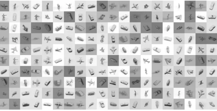
Figure 2.4: Visualizations of the graphs G∗, G
M and GN for a randomly chosen 250 test
examples from MNIST for themL = 100case. As implied through the relation defined in (2.7) and discussed in detail in Section 2.2.3, when we regularize N to become the identity matrix: i) G∗ becomes a biregular graph, ii) G
M turns into a disconnected graph of n m/n-regular
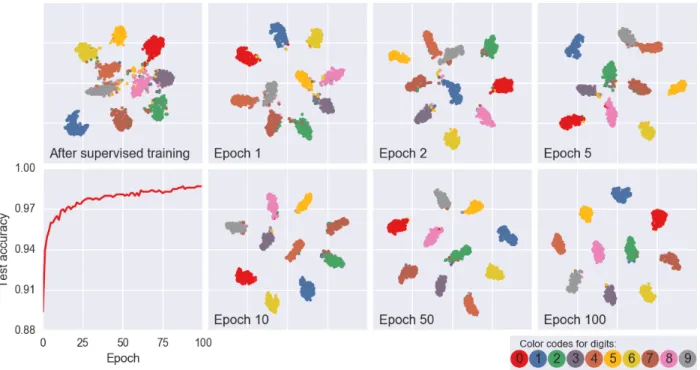
subgraphs, iii)GN turns into a disconnected graph ofn nodes having self-loops only (self-loops are not displayed for the sake of clarity), and automatically iv) B becomes the optimal embedding of M. Color codes denote the ground-truths for the examples. This figure is best viewed in color.
Figure 2.4 shows a visualization of the realization of the graph-based approach described in this chapter using real predictions for the MNIST dataset. After the supervised training, in the bipartite graph G∗ (defined by B), most of the examples are connected to multiple
output nodes at the same time. In fact, the graph between the examples GM (inferred by
M = BBT) looks like a sea of edges. However, thanks to supervised training step, some of these edges are actually quite close to the numerical probability value of 1. Through a scalable regularization objective, which is defined on the graph between the output nodes
GN (inferred by N = BTB), stronger edges are implicitly propagated in graph GM. In other words, as hypothesized, when N turns into the identity matrix, G∗ closes to be a
biregular graph and GM closes to be a disconnected graph of n m/n-regular subgraphs. As
implied through the relation defined in (2.7) and discussed in detail in Section 2.2.3, we expect B to automatically become the optimal embedding of M. Figure 2.5 presents the t-SNE [38] visualizations of the embedding spaces inferred by B. t-SNE is a popular method creating two-dimensional maps from data with thousands of dimensions. Recently, it has become widespread in the field of machine learning to explore high-dimensional data [66]. For semi-supervised and unsupervised settings, well-separated clusters on these two-dimensional maps indicate the quality of the obtained latent representation. However, the distances between well-separated clusters in a t-SNE plot may have no further meaning [66]. As clearly observed from Figure 2.5, as the unsupervised regularization exploits the unlabeled data, clusters become well-separated and simultaneously the test accuracy increases.
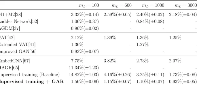
Table 2.3 summarizes the semi-supervised test accuracies observed with four different mL settings. Results of a broad range of recent existing solutions are also presented for comparison. These solutions are grouped according to their approaches to semi-supervised learning. While [28], [52], [37] employ autoencoder variants, [42], [41] and [56] adopt adversarial training, [67] and [65] are another graph-based methods. To show the baseline of the unsupervised regularization step in our framework, the performance of the network after the supervised training is also given. For MNIST, GAR outperforms existing graph-based methods and all the contemporary methods other than some cutting-edge approaches that use generative models.
Figure 2.5: t-SNE visualization of the embedding spaces inferred byB for a randomly chosen 2000 test examples for the mL = 100 case. Color codes denote the ground-truths for the examples. Note the separation of clusters from epoch 0 (right after supervised training step) to epoch 100 of the unsupervised training. For reference, accuracy for the entire test set of 10000 examples is also plotted with respect to the unsupervised training epochs. This figure is best viewed in color.
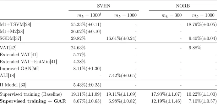
2.3.3.2 SVHN and NORB
SVHN and NORB datasets are both used frequently in recent literature on semi-supervised classification benchmarks [18, 28, 33, 37, 41, 42, 56]. Either dataset represents a significant jump in difficulty for classification when compared to the MNIST dataset. Table 2.4 summarizes the semi-supervised test accuracies observed on SVHN and NORB. For SVHN experiments, 1000 labeled examples have been randomly chosen with stratification among 73,257 training examples. Two experiments are conducted where the SVHNextra set (an additional training set including 531,131 more samples) is either omitted from the unsupervised training or not. The same batch ratio has been used in both experiments as bL = 96, bU = 32.
Table 2.3: Benchmark results of the semi-supervised test accuracies on MNIST for few labeled samples, mL∈ {100,600,1000,3000}. Results of a broad range of recent existing solutions are also presented for comparison. The last row demonstrates the benchmark scores of the proposed framework in this chapter.
mL = 100 mL= 600 mL= 1000 mL= 3000 M1+M2[28] 3.33%(±0.14) 2.59%(±0.05) 2.40%(±0.02) 2.18%(±0.04) Ladder Network[52] 1.06%(±0.37) - 0.84%(±0.08) -AGDM[37] 0.96%(±0.02) - - -VAT[42] 2.12% 1.39% 1.36% 1.25% Extended VAT[41] 1.36% - 1.27% -Improved GAN[56] 0.93%(±0.07) - - -EmbedCNN[67] 7.75% 3.82% 2.73% 2.07% HAGR[65] 11.34%(±1.23) - -
-Supervised training (Baseline) 14.82%(±1.03) 4.16%(±0.26) 3.25%(±0.11) 1.73%(±0.08)
Supervised training + GAR 1.56%(±0.09) 1.15%(±0.07) 1.10%(±0.07) 0.93%(±0.05)
On the other hand, for NORB experiments, to follow the previously published works reporting their results on the NORB dataset [28, 37] using 1000 labeled examples and to further create a more challenging scenario using less number of labeled examples, 2 different settings have been used for the number of labeled examples, i.e. mL={300,1000} with the same batch ratio of bL= 32, bU = 96, where labeled examples have been randomly chosen with stratification. Both results are included for comparative purposes.
Deep generative approaches [18, 28, 33, 37, 41, 42, 52, 56] have gained popularity especially over the last two years for semi-supervised learning and achieved superior per-formance for the problems in this setting in spite of the difficulties in their training. As it requires no additional work in calculating the reconstruction error (as in autoencoder based methods [28, 37, 52]) or implementing a zero-sum game mechanism (as in GAN based methods [41, 42, 56]), GAR is natural for the classification framework on neural networks and it is therefore a low-cost and efficient competitor for generative approaches and achieves
comparable performance with these state-of-the-art models while statistically significantly outperforming all existing graph-based methods. Most importantly, GAR is open to further improvements with standard data enhancement techniques such as augmentation, ensemble learning.
Table 2.4: Benchmark results of the semi-supervised test accuracies on SVHN and NORB. Results of a broad range of most recent existing solutions are also presented for comparison. The last row demonstrates the benchmarks for the proposed framework in this chapter.
SVHN NORB mL = 1000† mL= 1000 mL= 300 mL= 1000 M1+TSVM[28] 55.33%(±0.11) - - 18.79%(±0.05) M1+M2[28] 36.02%(±0.10) - - -SGDM[37] 29.82% 16.61%(±0.24) - 9.40%(±0.04) VAT[42] 24.63% - - 9.88% Extended VAT[41] 5.77% - - -Extended VAT+EntMin[41] 4.28% - - -Improved GAN[56] 8.11%(±1.30) - - -ALI[18] - 7.42%(±0.65) - -ΠModel [33] 5.43%(±0.25) - -
-Supervised training (Baseline) 19.11%(±1.09) 19.11%(±1.09) 17.93%(±1.07) 10.22%(±1.00)
Supervised training + GAR 8.67%(±0.65) 6.98%(±0.82) 12.19%(±1.46) 7.10%(±0.57)
†
This column presents the results obtained when SVHNextraset is omitted from the unsupervised training. Unless otherwise specified, reported results for other approaches are assumed to represent this scenario.
2.3.3.3 Effects of Hyperparameters
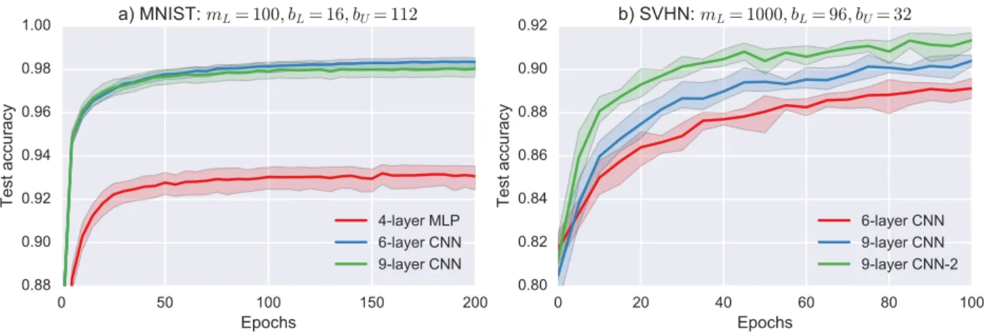
Figure 2.6 presents the test accuracy curves with respect to the unsupervised training epochs obtained using different models. The proposed unsupervised regularization improves the test accuracy in all models. However, the best case depends on the chosen model specifications.
0 50 100 150 200 Epochs 0.88 0.90 0.92 0.94 0.96 0.98 1.00 Test accuracy a) MNIST: mL= 100, bL= 16, bU= 112 4-layer MLP 6-layer CNN 9-layer CNN 0 20 40 60 80 100 Epochs 0.80 0.82 0.84 0.86 0.88 0.90 0.92 Test accuracy b) SVHN: mL= 1000, bL= 96, bU= 32 6-layer CNN 9-layer CNN 9-layer CNN-2
Figure 2.6: Test accuracies obtained using different models with respect to unsupervised training epochs. a) On the left, MNIST results are given for the settings that mL = 100 and bL = 16, bU = 112 and b) On the right, SVHN results are given for the settings that mL = 1000andbL= 96, bU = 32. Model specifications are given in Table 2.2. Shaded regions show the 0.95 confidence interval.
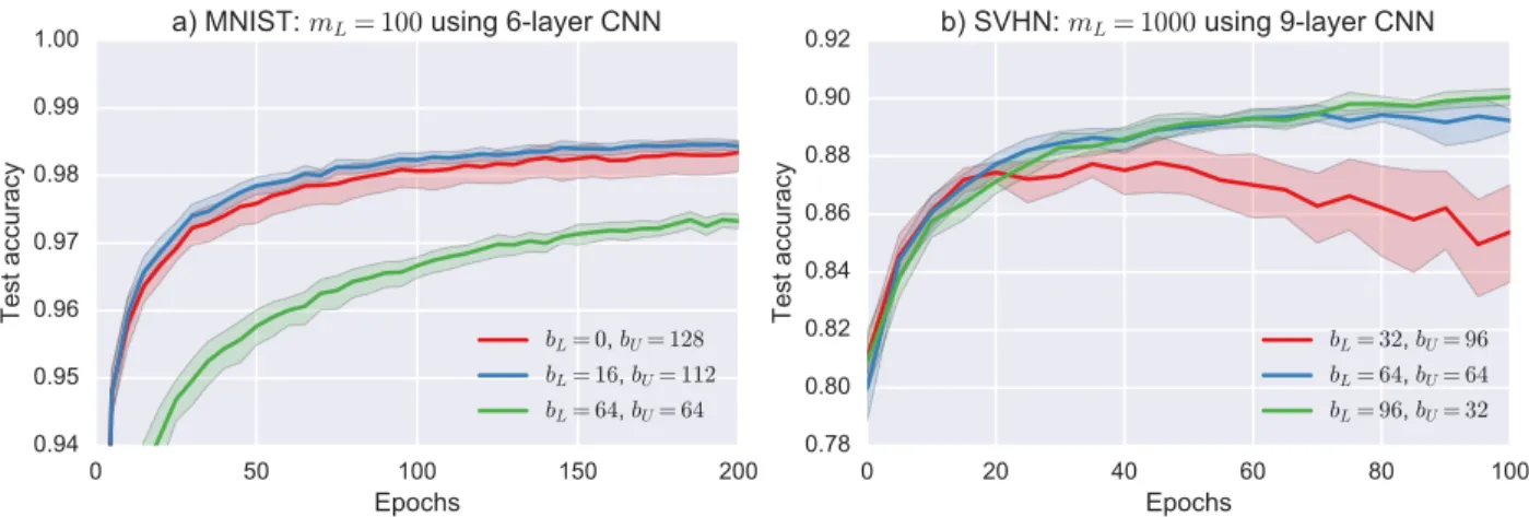
The labeled/unlabeled data ratio of unsupervised training batches is the most critical hyperparameter of the proposed regularization. Figure 2.7 visualizes the effect of this ratio for MNIST and SVHN datasets. These two datasets have different characteristics. MNIST dataset has a lower variance among its samples with respect to SVHN. As a result, even when the labeled examples introduced to the network during the supervised training are not blended with the unsupervised training batches, i.e. bL = 0, this does not affect the performance dramatically. However, for the SVHN dataset, reducing the bL proportion of the unsupervised training batches significantly affects the accuracy and further decrease of bL reduces the stability of the regularization.
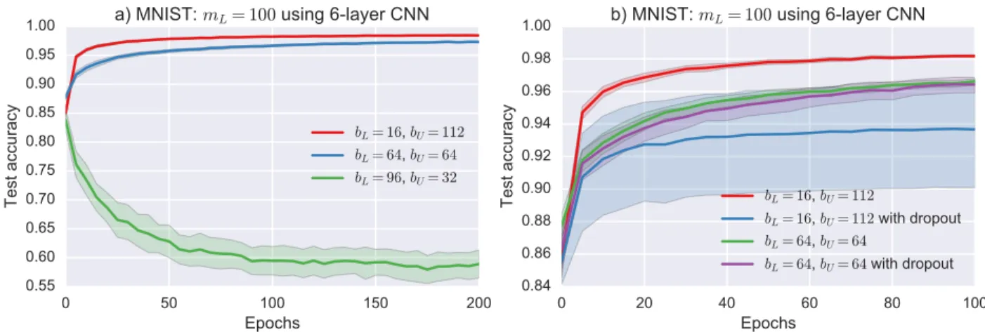
One can also observe another phenomenon through the MNIST results in Figure 2.7. That is, as bL approaches mL, the generalization of the model reduces. This effect can be better observed in Figure 2.8 including a further step, i.e. bL= 96 when mL = 100. Since the same examples start to dominate the batches of unsupervised regularization, overfitting occurs and ultimately test accuracy significantly reduces. Figure 2.8 also presents the effect
0 50 100 150 200 Epochs 0.94 0.95 0.96 0.97 0.98 0.99 1.00 Test accuracy
a) MNIST: mL= 100 using 6-layer CNN
bL= 0, bU= 128 bL= 16, bU= 112 bL= 64, bU= 64 0 20 40 60 80 100 Epochs 0.78 0.80 0.82 0.84 0.86 0.88 0.90 0.92 Test accuracy b) SVHN: mL= 1000 using 9-layer CNN bL= 32, bU= 96 bL= 64, bU= 64 bL= 96, bU= 32
Figure 2.7: The effect of bL/bU ratio for MNIST and SVHN datasets. Shaded regions show the 0.95 confidence interval.
of applying dropout during the unsupervised regularization. Dropping out the weights the during unsupervised training dramatically affects the accuracy. This effect is more obvious when bL is smaller. Hence, for the experiments, we removed the dropouts from the models specified in Table 2.2 during the unsupervised training.
The effects of regularization coefficients are presented in Figure 2.9 for the MNIST dataset. Part (a) of the figure visualizes the case whencF is held constant, but the ratio of cα/c
β changes. And part (b) of the figure illustrates the case when cα/cβ is held constant, but cF changes. We can say that as long ascα ≥cβ, the ratio ofcα/cβ does not affect the accuracy significantly. Furthermore, the value of cF is not so critical (close performances both with cF = 1e−6 andcF = 1e−15) unless it is too big to distort the regularization. Therefore, we can say that the proposed unsupervised regularization term is considerably robust with respect to the coefficients cα, cβ andcF. This can also be seen through the fact that we have applied the same coefficients for the experiments of all three datasets.
0 20 40 60 80 100 Epochs 0.84 0.86 0.88 0.90 0.92 0.94 0.96 0.98 1.00 Test accuracy
b) MNIST: mL= 100 using 6-layer CNN
bL= 16, bU= 112 bL= 16, bU= 112 with dropout bL= 64, bU= 64 bL= 64, bU= 64 with dropout 0 50 100 150 200 Epochs 0.55 0.60 0.65 0.70 0.75 0.80 0.85 0.90 0.95 1.00 Test accuracy
a) MNIST: mL= 100 using 6-layer CNN
bL= 16, bU= 112 bL= 64, bU= 64 bL= 96, bU= 32
Figure 2.8: The effects of a) on the left, choosing bL ≈ mL and b) on the right, applying dropout during the unsupervised training on MNIST dataset. Note that the figures show different ranges of training epochs, i.e. 200 vs. 100. Shaded regions show the 0.95 confidence interval. 0 50 100 150 200 Epochs 0.84 0.86 0.88 0.90 0.92 0.94 0.96 0.98 1.00 Test accuracy a) MNIST: cF= 1e−6 cα= 3, cβ= 1 cα= 1, cβ= 1 cα= 1, cβ= 2 0 50 100 150 200 Epochs 0.4 0.5 0.6 0.7 0.8 0.9 1.0 Test accuracy b) MNIST: cα= 3, cβ= 1 cF= 1e−15 cF= 1e−6 cF= 1e−5
Figure 2.9: The effects of a) cα/c
β and b) cF on MNIST dataset. Shaded regions show the 0.95 confidence interval. The size of green shaded regions implies the instability of the model when using the specified settings as the obtained accuracy varies drastically per epoch.
CHAPTER 3: AUTO-CLUSTERING OUTPUT LAYER: AUTOMATIC LEARNING OF LATENT ANNOTATIONS IN NEURAL NETWORKS1
Combinations of supervised and unsupervised learning have resulted in many fruitful developments throughout the machine learning literature. Among many achievements, unsupervised feature learning where unsupervised training is used as a pretraining stage for initializing hidden layer parameters [22], was the first method to succeed in the training of fully connected deep architectures and played a key role in igniting the third wave of machine learning research by creating a paradigm shift we now call deep learning [19].
In current literature, different kinds of approaches exist to combine supervised and unsupervised learning. In this context, semi-supervised is frequently used to specify certain applications where a large number of observations exist with only a small subset having ground-truth labels. Solutions suggested for these applications seek ways of exploiting the unlabeled data to improve the model generalization. There have been significant developments recently in this field. Following the introduction of Bayesian inference to the conventional autoencoder architecture [29, 53], these variational autoencoders have been proven to make deep generative models highly competitive for semi-supervised learning [28, 37]. Virtual adversarial training [42] motivated by Generative Adversarial Nets [20] and the denoising autoencoder variant named Ladder networks [61] have also been successfully employed for semi-supervised learning problems [52]. On the other hand, in the previous chapter, we have proposed a scalable and efficient graph-based method that is natural for the classification framework on neural networks as it requires no additional work calculating the reconstruction 1This chapter has been submitted to peer-reviewed IEEE Transactions on Neural Networks and Learning
error (as in autoencoder based methods) or implementing zero-sum game mechanism (as in adversarial training based methods) and we reported competitive performance with respect to other approaches.
In this chapter, we consider a different kind of semi-supervised setting in which a coarse level of labeling (e.g. tree, flower) is available for all observations, but the model still needs to learn a fine level of latent annotations, which are previously unknown to the user (e.g. maple, rose), for each one of them. Provided labeling can be interpreted as parent-class information and latent annotations to be explored can be conceived as the sub-classes. Since partial supervision does not involve any explicit information, sub-class exploration is considered an unsupervised task. Therefore, the overall learning procedure can be considered semi-supervised. For clarification, let us assume that we are given a dataset of hand-written digits such as MNIST [35] where the overall task is complete categorization of each digit, but the only available supervision is whether a digit is smaller or greater than 5, as visualized in Figure 3.1. While being trained to categorize each example as a member of parent-classes, {0,1,2,3,4} or {5,6,7,8,9}, the model also needs to learn to distinguish the digits, sub-classes under the same parent from each other. Since provided labeling involves no explicit information about the difference between the samples of digit 0 and the samples of digit 1, their separation is performed as an unsupervised task. As we use partial supervision to help overall categorization, the entire procedure is semi-supervised.
Outside the neural network literature, the learning of latent variable models when supervision for more general classes than those of interest is provided has previously been studied. In the natural language processing (NLP) field, following the introduction of Latent Dirichlet Allocation (LDA), a completely unsupervised algorithm that models each document as a mixture of topics [11], several modifications have been proposed to incorporate supervision [10, 32, 48, 49]. These ideas have also been extended for simultaneous image classification and annotation [51, 64].
Classification (Partial Supervision)
Clustering (Latent Annotations)
Figure 3.1: Particular semi-supervised setting discussed in this chapter. That is, a coarse level of labeling is available for all observations but the model has to learn a fine level of latent annotation for each one of them. We propose a novel approach that considers these problems as simultaneously performed supervised classification (per provided parent-classes) and unsupervised clustering (within each parent) tasks and devise a framework to enable a neural network to learn the latent annotations in this partially supervised setup.
From the viewpoint of parent/sub-class interpretation of the provided supervision and latent annotations, an analogy can be established between the semi-supervised problems discussed in this chapter and the hierarchical classification tasks in the literature. Hierarchical classification has previously been studied in neural networks [68]; however, proposed ap-proaches consider the completely supervised case where every observation in the dataset has a parent-class label but only a few of them also have additional sub-class labels. The literature about hierarchical classification is scattered across very different application domains such as text categorization, protein function prediction, music genre classification and image classification [26].
Given partial supervision, latent annotation learning is also a common problem in these domains as well as in exploratory scientific research such as in medicine and genomics [5],
as the tasks in these domains naturally involve both already-explored (hence labeled) classes and extraction of not-yet-explored (hence hidden) patterns. In this chapter, we propose a novel approach that considers these problems as simultaneously performed supervised classification (per provided parent-classes) and unsupervised clustering (within each parent) tasks and devise a framework to enable a neural network to learn the latent annotations in this partially supervised setup. This framework involves a novel output layer modification called the auto-clustering output layer (ACOL) that allows concurrent classification and clustering tasks where clustering is performed according to the Graph-based Activity Regularization (GAR) technique proposed in the previous chapter. ACOL duplicates the softmax nodes at the output layer and GAR allows for competitive learning between these duplicates in a traditional error-correction learning framework.
This chapter is organized as follows. The next section briefly summarizes the activity regularization proposed in the previous chapter which we adopt as the objective of the unsupervised portion of the training. In the third section, we describe the proposed output layer modification and its integration with the GAR technique and experimental results are presented in the fourth section.
3.1 Related Work
GAR is a scalable and efficient graph-based approach which was originally proposed for the classical type of semi-supervised learning problems where a large number of observations with only a small subset of corresponding labels exist. In this chapter, we adopt the same regularization terms and show that these terms can be employed to reveal the latent annotations in a supervised setup through ACOL. After describing ACOL, Section 3.2.2 describes how ACOL is integrated with the GAR technique.