North Carolina Agricultural and Technical State University North Carolina Agricultural and Technical State University
Aggie Digital Collections and Scholarship
Aggie Digital Collections and Scholarship
Theses Electronic Theses and Dissertations
2011
Thermal Characterization Of Carbon Composites
Thermal Characterization Of Carbon Composites
Jr. Darryl BakerNorth Carolina Agricultural and Technical State University
Follow this and additional works at: https://digital.library.ncat.edu/theses
Recommended Citation Recommended Citation
Baker, Jr. Darryl, "Thermal Characterization Of Carbon Composites" (2011). Theses. 13. https://digital.library.ncat.edu/theses/13
This Thesis is brought to you for free and open access by the Electronic Theses and Dissertations at Aggie Digital Collections and Scholarship. It has been accepted for inclusion in Theses by an authorized administrator of Aggie Digital Collections and Scholarship. For more information, please contact [email protected].
THERMAL CHARACTERIZATION OF CARBON COMPOSITES
by
Darryl Douglas Baker, Jr.
A thesis submitted to the graduate faculty
in partial fulfillment of the requirements for the degree of MASTER OF SCIENCE
Department: Mechanical Engineering Major: Mechanical Engineering Major Professor: Dr. Messiha Saad
North Carolina A&T State University Greensboro, North Carolina
School of Graduate Studies
North Carolina Agricultural and Technical State University
This is to certify that the Master’s Thesis of
Darryl Douglas Baker, Jr.
has met the thesis requirements of
North Carolina Agricultural and Technical State University Greensboro, North Carolina
2011
Approved by:
________________________________ ________________________________ Dr. Messiha Saad Dr. John Kizito
Major Professor Committee Member
________________________________ ________________________________ Dr. Frederick Ferguson Dr. Samuel Owusu-Ofori
Committee Member Department Chairperson
___________________________________ Dr. Sanjiv Sarin
Interim Associate Vice Chancellor for Research and Graduate Dean
DEDICATION
I dedicate this thesis to my wonderful friends and family. Without you, I would not be where I am today. When I felt like I was at the lowest point of my life, you were there to pick me up and motivate me to keep striving for excellence. Thank you for all you have done for me.
BIOGRAPHICAL SKETCH
Darryl Douglas Baker, Jr. was born May 24, 1985 to Darryl and Belinda Baker in Salzkotten, Germany. He spent majority of his childhood in Savannah and Columbus, Georgia. Upon graduation from William H. Spencer High School in 2003, he attended Fort Valley State University where he received a Bachelor of Science in Mathematics in spring 2006. After completing his first formal degree, he attended Georgia Institute of Technology where he received a Bachelor of Science in Mechanical Engineering in fall 2008. In addition, he is a certified Engineer-In-Training in the State of Georgia. Mr. Baker is a candidate for the Master of Science in Mechanical Engineering.
ACKNOWLEDGMENTS
I would like to show appreciation to my advisor, Dr. Messiha Saad, for giving me the opportunity to work beside him, and sharing his knowledge to help me grow not only as an engineer but as a person. I would also like to acknowledge Dr. Mannur Sundaresan for assisting me throughout my experience at North Carolina A&T State University, and Dr. John Kizito and Dr. Frederick Ferguson for taking time out of their busy schedules to serve on my thesis committee.
In addition, I would like to acknowledge Dr. Marc-Antonie Thermitus from Anter Corporation, and Mr. John Kelly from NETZSCH Instruments for sharing their knowledge of the flash method and differential scanning calorimetry. I would like to acknowledge Oak Ridge National Laboratory’s High Temperature Materials Laboratory sponsored by the U. S. Department of Energy, Office of Energy Efficiency and Renewable Energy, Vehicle Technologies Program. Also I would like to acknowledge NASA – URC (Grant# NNX09AV08A). Last but not the least, I would like to thank my lovely wife, Regina, for helping with the editing process.
TABLE OF CONTENTS
LIST OF FIGURES ... viii
LIST OF TABLES ...x
NOMENCLATURE ... xi
ABSTRACT ... xiii
CHAPTER 1 INTRODUCTION...1
CHAPTER 2 REVIEW OF THEORY ...4
2.1 Thermal Properties of Composite Materials...7
2.2 Examined Carbon Composites ...8
CHAPTER 3 EXPERIMENTIAL TECHNIQUES ... 12
3.1 The Flash Method ... 12
3.1.1 Experimental Apparatus ... 19
3.1.2 Test Specimen Preparation ... 20
3.1.3 Experimental Procedure ... 21
3.2 Differential Scanning Calorimetry ... 22
3.2.1 Experimental Apparatus ... 26
3.2.2 Test Specimen Preparation ... 28
CHAPTER 4 RESULTS AND DISSCUSSIONS ... 32 4.1 Thermal Diffusivity... 32 4.2 Specific Heat... 43 4.3 Thermal Conductivity ... 47 CHAPTER 5 CONCLUSION ... 51 REFERENCES ... 53
LIST OF FIGURES
FIGURE PAGE
2.1. T300 Carbon-Carbon Composite...9
2.2. Graphitized T300 Carbon-Carbon Composite ... 10
2.3. AS4/3501-6 Carbon-Epoxy Composite ... 11
3.1. Schematic of the Flash Method ... 13
3.2. Characteristic Thermogram for the Flash Method ... 14
3.3. Thermogram Displaying the Half-Time ... 17
3.4. FlashLine™ 2000 Thermal Properties Analyzer ... 19
3.5. DSC 200 F3 Maia® Differential Scanning Calorimeter ... 27
3.6. Cross Section View DSC 200 F3 Maia® ... 28
3.7. Crucible Placed on the Heat Flux Sensor ... 30
4.1. Transverse Thermal Diffusivity of AS4/3501-6 Composite ... 32
4.2. Transverse Thermal Diffusivity of T300 Composite ... 33
4.3. Transverse Thermal Diffusivity of Graphitized T300 Composite... 34
4.4. Transverse Thermal Diffusivity Comparison of T300 Composites ... 35
4.5. Comparison of the AS4/3501-6 Composite Thermograms to the Theoretical Model ... 40
4.6. Comparison of the T300 Composite Thermogram to the Theoretical Model ... 40
4.7. Comparison of the Graphitized T300 Composite to the Theoretical Model ... 41
4.8. AS4/3501-6 Composite Thermal Diffusivity Comparison ... 42
4.9. Graphitized T300 Composite Thermal Diffusivity Comparison ... 43
4.10. Specific Heat of the Sapphire Reference ... 44
4.11. Specific Heat of the AS4/3501-6 Composite ... 44
4.12. Specific Heat of the T300 Composite ... 45
4.13. Specific Heat of the Graphitized T300 Composite ... 45
4.14. T300 Composite Specific Heat Comparison ... 46
4.15. Thermal Conductivity of the AS4/3501-6 Composite ... 47
4.16. Thermal Conductivity of the T300 Composite ... 48
4.17. Thermal Conductivity of the Graphitized T300 Composite... 48
LIST OF TABLES
TABLE PAGE
3.1. Cowan’s Correction Factor ... 18
3.2. Flash Method Test Specimens ... 21
3.3. DSC Test Specimens... 29
4.1. Half-Time of the Test Materials ... 36
4.2. Constant kx for Various Percent Rises ... 37
4.3. Thermal Diffusivity Validation of AS4/3501-6 Composite ... 37
4.4. Thermal Diffusivity Validation of T300 Composite ... 38
4.5. Thermal Diffusivity Validation of Graphitized T300 Composite ... 39
NOMENCLATURE
ax thermal diffusivity in the in-plane direction, m2/s
ay thermal diffusivity in the transverse direction, m2/s
A cross sectional area, m2
Cp constant pressure specific heat, kJ/kgK
Cp,Ref specific heat of the reference, kJ/kgK
dH change in enthalpy, kJ
dQ/dt heat flux, W
dT temperature difference, K
E DSC Calibration constant
̇ heat generation rate, W/m3
g depth, m
H enthalpy, kJ
k thermal conductivity, W/mK
K diffusivity correction factor
Kx diffusivity constant
kmix(max) maximum thermal conductivity of composite material, W/mK
kmix(min) minimum thermal conductivity of composite material, W/mK
kn thermal conductivity of the composite component, W/mK
mRef mass of the reference, g
m mass of the sample, g
Q pulse of radiant energy, heat transfer, kJ
̇ local heat flux, W
T temperature, °C or K
t time, s
T0 initial temperature, °C or K
t1/2 half-time, s
Tm maximum temperature of the rear surface, °C or K
V dimensionless parameter
Vn volume fraction of the composite component
α thermal diffusivity, m2/s
αcorrected corrected diffusivity value
αn thermal diffusivity of the composite component, m2/s
Δti temperature ratio
(ρc)eff effective volumetric heat capacity, kJ/m3K
ρ density, kg/m3
ρn density of the composite component, kg/m3
ABSTRACT
Baker, Darryl Douglas, Jr. THERMAL CHARACTERIZATION OF CARBON COMPOSITES (Major Advisor: Dr. Messiha Saad), North Carolina Agricultural and Technical State University.
Thermophysical properties of materials such as, thermal conductivity, diffusivity, and specific heat, are very important in engineering design process. For example, thermal conductivity plays a critical role in the performance of materials in high temperature applications and it is essential in the selection of materials when optimum performance is desired. Other thermophysical properties, such as thermal diffusivity and specific heat capacity, play significant roles in design application as they determine safe operating temperature, form process control characteristics, and quality conditions in manufacturing plants.
The objective of this research was to determine the thermal properties of carbon composite materials. The materials of interest to this analysis were carbon-carbon and carbon-epoxy composites. The carbon-carbon composites tested were produced by the resin transfer molding process using T300 PAN based carbon fiber and PT-30 cyanate ester matrix. In contrast, the carbon-epoxy composite tested consisted of unidirectional continuous AS4 carbon fiber and 3501-6 amine cured epoxy resin.
Following standard ASTM E1461, the flash method was used to measure the thermal diffusivity of the carbon composites. In addition, a differential scanning calorimeter was used in accordance with the ASTM E1269 standard to determine the
specific heat. The thermal conductivity of the carbon composites was determined using the measured values of their thermal diffusivity and specific heat, respectively.
CHAPTER 1 INTRODUCTION
As today’s technology continues to develop at a rate that was once unimaginable, the demand for new materials that will outperform traditional materials also increases at an alarming rate. To meet these challenges, monolithic materials are being combined to develop new unique materials called composites. The formation of composites provides properties unobtainable separately with either constituent. Besides improvements in the mechanical properties such as tensile strength, stiffness, and fatigue endurance, materials must retain functionality at much higher operating temperatures than before. Due to extreme temperatures, material properties may alter in operation, resulting in severely reduced properties, which may lead to catastrophic failures during usage. Thermophysical properties play a significant role in design applications, determining safe operating temperatures, process control characteristics, and quality assurance of these materials.
In the past, countless number of research have been done to predict and determine the mechanical properties of composites on both a microscopic and a macroscopic scale. However, today mechanical properties can be studied either experimentally or analytically as prescribed by ASTM standards. ASTM established specific test methods for the mechanical characterization of unidirectional lamina [1]. Compared to mechanical properties, few efforts have been made in developing testing standards strictly for thermophysical properties of composites. To measure the thermophysical properties of a composite, one must utilize a proven technique developed for a homogeneous material,
with the results when substantial inhomogeneity and anisotropy are present in a composite material.
Current methods for measuring the thermophysical properties are the flash method, the thermal wave interferometry method, and numerous thermographic methods. The flash method is viewed as the reference technique because it is the only method covered by an ASTM standard [2]. The thermal conductivity can be indirectly determined using the measured thermal diffusivity, density, and specific heat capacity of the material.
North Carolina A&T State University has a strong experience in composite materials. In 1988, the Center for Composite Material Research (CCMR) was established. The CCMR is recognized for research excellence in composite materials with research supported by the Office of Naval Research, National Science Foundation, and Army Research Office [3]. The focus of the CCMR is developing state-of-the-art composites and processing techniques for applications in the aerospace, marine, and civil infrastructures. Mechanical properties are predicted using machinery such as a Dynamic Mechanical Analyzer (DMA 7), and hydraulic fracture testing machinery.
The objective of this research is to determine the thermophysical properties of carbon composites, and establish a reliable means of measuring the thermophysical properties of materials produced in the CCMR. Specifically, the thermal conductivity of the carbon composites will be determined using the diffusivity results obtained from the flash method combined with measurements of specific heat capacity obtained from a differential scanning calorimeter.
The materials of interest to this analysis include carbon-carbon and carbon-epoxy composites. The tested carbon-carbon composites were produced by the resin transfer molding process using T300 PAN based carbon fiber and PT-30 cyanate ester. In contrast, the carbon-epoxy composite tested consisted of unidirectional continuous AS4 carbon fiber and 3501-6 amine cured epoxy resin. The thermal testing techniques used in this research will complement the mechanical testing techniques already established in the CCMR, and provide data to the scientific community.
CHAPTER 2 REVIEW OF THEORY
The rate of conduction is affected by the temperature difference across the medium with a larger temperature difference resulting in a higher rate of heat transfer. In addition, the geometry and material of the medium plays a significant role in the rate of conduction. The rate of heat conduction through the plane is proportional to the temperature difference across the plane and the surface area, but is inversely proportional to the thickness. Taking the material property into consideration, thermal conductivity k,
can be related to the rate of heat flow as follows [4]:
̇
(2.1)
where ̇ is the local heat flux, A is the cross sectional area, dT is temperature difference, and dx is the material thickness. The previous equation is known as the Fourier’s Law of
Heat Conduction, named after the French mathematician Joseph Fourier. Performing an energy balance, the general heat conduction equation can be developed as the following [4]:
̇
(2.2)
and then simplified using the Laplacian operator to the following [4]:
̇
(2.3)
The equation above is known as the Biot equation. Further reducing the Fourier-Biot equation to one-dimensional analysis leads to the following [4]:
̇
(2.4)
Many scientists view the Fourier’s Law of Heat Conduction as the defining equation for thermal conductivity. The thermal conductivity of a material can be defined as the rate of heat transfer through a unit thickness of the material per unit area per unit temperature difference [4]. Thermal conductivity can simply be defined as the measure of the ability of a material to conduct heat due to a temperature gradient in that material [5]. In Equation (2.1), the thermal conductivity has a negative value. This negative value of denotes that heat is transferred in the direction of decreasing temperature [6].
The unit of thermal conductivity in SI is Watts per meters per degree Kelvin (W/m·K). Because Fourier’s Law of Heat Conduction contains a temperature gradient rather than a temperature, degree Kelvin may be replaced with degree Centigrade (W/m·˚C). It can be also instructive to view thermal conductivity in the form (W·m)/ (m2·K), which has the interpretation that thermal conductivity is the rate of heat transfer through the unit thickness of a material per unit surface area per unit temperature difference.
Materials that conduct heat well have high values of thermal conductivity. These materials are known as conductors. On the opposite end of the spectrum are insulators. Insulators do not conduct heat well and have comparatively low values for thermal conductivity. In general, thermal conductivity is strongly depended on temperature. In addition, pressure and material density is known to have an influence on thermal conductivity.
Thermal diffusivity can be defined as “the quantity that measures the change in temperature produced in unit volume of the material by the amount of heat that flows in unit time through a unit area of a layer of unit thickness with unit temperature difference between its faces” [7]. Thermal diffusivity is described as the “thermal inertia of materials” [5]. It measures the ability of a material to conduct heat transfer through itself relative to its ability to store thermal energy. Materials with large values of thermal diffusivity will equilibrate to their thermal environment at a rapid rate, while a material with a small value of thermal diffusivity will respond less rapidly, taking longer to achieve equilibrium.
Thermal conductivity and diffusivity are not independent quantities. They are related through the following relationship:
(2.5)
where ρ is the density, and cp is the specific heat. Since thermal conductivity represents
the rate at which a material conducts heat, and the volumetric heat capacity, ρcp,
represents the material storage capacity of energy per unit volume, thermal diffusivity is viewed as the ratio of the heat conduction of the material to the heat stored per unit volume.
The product of the density ρ and specific heat cp is known as the volumetric heat
capacity. The volumetric heat capacity, ρcp, signifies the ability of a given volume of
material to store energy while undergoing a given temperature change. A commonly used unit for volumetric heat capacity is Joule per meter cubed per Kelvin, J/(m³·K).
2.1 Thermal Properties of Composite Materials
According to A. Salazar [7], the Fourier’s Law of Heat Conduction and the general heat conduction equation are not applicable for composite materials. Salazar explains that due to the heterogeneous nature of the materials the thermal properties are discontinuous functions of the location making those theories not valid. When considering composites Salazar suggests using the concept of effective properties, where properties of the equivalent homogeneous materials are used on a volume basis. Effective properties led to the rule of mixtures. The rule of mixtures states that “the properties of the composites are the weighted average of the properties of its individual components” [8]. Using the mixture rule, the effective volumetric heat capacity of a composite made of two components leads to the following [7]:
(2.6)
where v1 and v2 are the volume fraction of each component the composite respectively,
and the summation, v1 + v2 = 1.
When examining the thermal conductivity of composite materials, Parrott and Stuckes [9] revealed that maximum thermal conductivity is achieved in-plane of the laminas using a comparison to electricity with parallel resistors. This assessment led to the following relationship [9]:
(2.7)
where kmix(max) is the maximum thermal conductivity of the composite material. However,
direction is comparable to resistors in series. The total conductivity is now the following [9]:
(2.8)
where kmix(min) is the minimum thermal conductivity of the composite material. Using
Equation (2.6), effective volumetric heat capacity, and the minimum and maximum thermal conductivity of the composites, a relationship can be developed to calculate the thermal diffusivity in both the in plane and transverse direction [7]:
(2.9) ( ) (2.10)
where αx is the thermal diffusivity in the in plane direction, and αy is the transverse
direction. In this research, the thermal diffusivity in the transverse direction is determined.
2.2 Examined Carbon Composites
The thermophysical properties of three carbon composite materials were investigated in the research. Two of the carbon composites examined consisted of a carbon fiber in a carbon matrix known as a carbon-carbon composite. The carbon-carbon composites were produced with the resin transfer molding (RTM) process. The additional
carbon composite was a unidirectional carbon-epoxy composite. The unidirectional carbon-epoxy composite was produced using the autoclave molding method.
The carbon-carbon composites [10] for which the thermophysical properties were obtained consisted of Thornel T-300 PAN-Based carbon fiber, and Primaset PT-30 cyanate ester resin. One of the examined carbon-carbon composite consisted of carbon fibers which were graphitized at 2500°C. The two carbon-carbon composites tested were 7-ply samples that were densified twice to achieve the desired density. The tested carbon-carbon composite are shown in Figures 2.1 and 2.2.
Figure 2.2. Graphitized T300 Carbon-Carbon Composite
The other carbon composite used in this research was a unidirectional, continuous carbon-epoxy laminate, AS4/3501-6, consisted of AS4 carbon fiber and 3501-6 amine cured epoxy resin, both produced by Hexcel Composites. The carbon-epoxy composite was an 8-ply laminate compiled of laminas alternating between 0° and 90° orientations. The AS4 carbon fiber used was a continuous, PAN based fiber that was surfaced treated to improve the fiber-to-resin interfacial bond strength, which met Hexcel aerospace specification HS-CP-5000 [11]. The 3501-6 epoxy resin provided low shrinkage during the curing process while maintaining excellent resistance to chemicals and solvent. AS4/3501-6 carbon-epoxy composite has a high gloss, smooth black finish, which is displayed in Figure 2.3.
CHAPTER 3
EXPERIMENTIAL TECHNIQUES
3.1 The Flash Method
In the late 1950s and 1960s there were renewed interests in developing new testing methods of determining the thermal conductivity and the thermal diffusivity of materials [12]. This interest was largely due to the progression made in the study of materials operating at elevated temperatures [13]. During this time period, advanced materials research laboratories were established by the U.S. government making material science a multidisciplinary research collaboration effort [14]. Numerous techniques existed that measured thermophysical properties in both steady-state and non-steady-state conditions. However, the amount of time required to attain reliable measurements, in addition to the large sample sizes required by former techniques, greatly increased the difficulty of performing measurements. Also, the difficulty of extending those methods to high temperature was proven to be a dilemma in high temperature technology. Parker, Jenkins, Butler, and Abbott [15] made progress regarding those issues in 1961 with an introduction of the Flash Method.
Since the introduction of the flash method, it has developed into one of the most widely used techniques for measuring the thermal diffusivity of various kinds of solids, and is a test method standard for thermal diffusivity [16]. This test method can be considered an absolute method of measurement, since no reference standards are
required. The technique has been adapted to measure the thermal diffusivity of various powders and liquids.
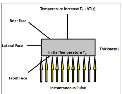
The flash method involves heating the front face of a small, cylindrical shaped sample by a short uniform energy pulse as displayed in Figure 3.1. A detector measures the temperature rise with respect to time on the rear face of the sample. By placing the sample into a tube furnace, temperature-dependent measurements can easily be carried out as well.
Figure 3.1. Schematic of the Flash Method
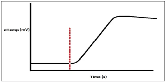
A data acquisition system records the change of temperature of the material with respect to time. This is known as the thermogram of the flash. The characteristic response of a flash method trial logged by the data acquisition system is displayed in Figure 3.2. The temperature change is measured with a infra read detector, therefore has the units of
trial. After the flash, the increase of the change of temperature with respect to the initial temperature is documented by the data acquistion system
Figure 3.2. Characteristic Thermogram for the Flash Method
Starting with Carslaw and Jeager’s [17] equation of temperature distribution within a thermally insulated solid of uniform thickness L, Parker et al. [15] derived the
mathematical expression to calculate thermal diffusivity (see APPENDIX for complete derivation):
∫ ∑ ( ) ∫
( (3.1)
where α is the thermal diffusivity of the material. When the pulse of radiant energy, Q, is instantaneously and uniformly adsorbed at a small depth given as g, on the front surface
at a distance x = 0, the initial conditions of the temperature distribution, T(x, t) at that
(3.2) (3.3) Substituting the initial conductions into the equation of temperature distribution within a thermally insulated solid of uniform thickness, it reduces to the following [15]:
[ ∑ ( )] (3.4) where ρ is the density and Cp is the specific heat capacity of the material. Since the
adsorption depth is a very small for opaque materials, the small angle approximation can be made [15]:
(3.5)
(3.6)
At the rear surface, where , the temperature distribution can be expressed by the following [15]: [ ∑ ( ) ] (3.7)
Parker et al.[15] defined two dimensionless parameters, V and ω as
(3.9) where Tm represents the maximum temperature at the rear surface. The combination of
Equations (3.7), (3.8) and (3.9) yields the following expression [15]:
1111111111111111111 1
∑
111111111111111(3.10)
By setting V to 0.5 in Equation (3.10), Parker determined ω to be 1.38. By substituting the value of ω in Equation (3.9), the thermal diffusivity can be written as [15]:
⁄ (3.11)
Equation (3.11) can be rewritten as [15]:
⁄ (3.12)
where ⁄ is the time required for the back surface to reach half of the maximum temperature rise. The value, ⁄ is also known as the half-time and can be seen in Figure 3.3. The advantage of the flash method is that only the thickness of the sample and its half-time is required to calculate the thermal diffusivity. Unfortunately, radiation heat losses are not taken into account. The flash method model is the ideal case assuming that heat flow is one dimensional, and that there is no heat lost from the surface of the test specimen. In addition, Parker et al. [15] assumed the pulse absorption on the front surface
was uniformed, and the pulse duration was infinitesimally short. This assumption ultimately made led to some controversy.
Figure 3.3. Thermogram Displaying the Half-Time [18]
Cowan [19] released a document that challenged the theoretical analysis of the Flash Method. Cowan questioned the applicability of the method at high temperatures due to thermal radiation or other losses from the surfaces. Cowan’s argument was based on the observation that the temperature did not remain constant once the maximum temperature was achieved after the pulse, but steadily dropped after the peak. Cowan used the ratio of the recorded temperatures at both the t1/2, and a multiple times the
half-time (with five and ten being the most commonly used multiples), then developed a correction factor that accounted for heat losses:
1111111111111111111111 111111111111111111(3.13)
where αcorrected is the corrected diffusivity value, and Kc is the Cowan’s correction factor.
The following formula was used to calculate the correction factor:
where the variable A through H are coefficients, and is the used temperature ratio. The value of each coefficient can be seen in Table 3.1.
Table 3.1. Cowan’s Correction Factor
Coefficients Δt5 Δt10 A -0.1037162. 0.054825246 B 1.2390400 0.166977610 C -3.9744330. -0.286034370. D 6.8887380 0.283563370 E -6.8048830. -0.134032860. F 3.8566630 0.024077586 G -1.1677990. 0.000000000 H 0.1465332 0.000000000
Expanding on Cowan’s findings, Clark and Taylor [20] developed an analytical correction that considered radiative losses by using ratios. Unlike Cowan’s approach, Clark and Taylor examined the thermogram before the maximum temperature was achieved, and used ratios of partial times rather than partial temperatures. The establish ratio for this correction was t0.75/t0.25, that is, “the time to reach 75% of the maximum
divide by the time to reach 25% of the maximum” [16]. The factor to correct for radiative losses using Clark and Taylor’s approach was computed using the following formula:
111 ⁄ (3.15) where KR is the correction factor. The thermal diffusivity determined using the flash
method can now be corrected using the following Equation (3.16).
111111111111111111111 (3.16) The Clark and Taylor’s correction was used in this research.
3.1.1 Experimental Apparatus
The apparatus used in the research was Anter Corporation’s FlashLine™ 2000 Thermal Properties Analyzer seen in Figure 3.4. The FlashLine™ 2000 determines the thermal diffusivity of materials using a high energy xenon discharge as the pulse source. In addition, the FlashLine™ 2000 has the capability to determine the specific heat capacity and thermal conductivity of the tested material. The thermal diffusivity can be measured from ambient temperature to 330°C with a coverage range of 0.001 to 10 cm2/s within an accuracy of 4% and repeatability of 2%. The FlashLine™ 2000 also meets ASTM testing standard E1461, the Standard Test Method for Thermal Diffusivity by the Flash Method.
The thermal property analyzer consists of the following: flash source, specimen holder, environmental enclosure, temperature response detector, and data acquisition system [16]. The flash source on The FlashLine™ 2000 is a xenon pulse source capable of generating a short duration pulse of substantial energy. A quadruple specimen holder houses the samples in a vacuum tight environmental enclosure as the experiment is executed. The temperature response detector provides a linear electrical output proportional to a small temperature rise by means of an InSb infrared detector. The data acquisition system must be prompt to ensure that time resolution in determining the half-time is at least 1% for the fastest the thermogram for which the system is qualified. To perform this task, the FlashLine™ 2000 employs a data acquisition system that is capable of pre-programmed, multiple speed logging within a single time period. This enables high-resolution logging prior to and during the rising portion of the thermogram, while low-resolution logging during the cool down of the sample [21].
3.1.2 Test Specimen Preparation
Test specimens were prepared to the shape of thin circular discs with a front surface area less than of the flash source. The diameter of the test specimens can range from as large as 30 mm to as small as 6 mm, with 10 to 12.5 mm being the norm. According to ASTM E1461, the thickness of the test specimens must be between 1 to 6 mm. The optimum thickness varies by the estimated thermal diffusivity, and is chosen so the half-time falls within the 10 to 1000 ms range. To achieve the desired dimension, the material was cut to the proper diameter using a drill press with a diamond plated drill bit, then milled to the desired thickness when necessary.
The faces of the specimens were flat and parallel within 0.5% of their thickness to prevent any un-uniformity is the pulse. This reduces the error of thermal diffusivity measurement due to measuring the thickness below 1%. A thin, uniform layer of graphite is applied to both faces of the specimens to improve the capability of absorbing the applied energy flash by reducing the reflectability of the specimen. Gold, platinum, aluminum, nickel, or silver and then a coat of graphite are frequently applied to translucent and transparent specimens. Specifications of the samples used in this experiment can be seen in Table 3.2.
Table 3.2. Flash Method Test Specimens Material Diameter (mm) Thickness (mm) Mass (g) Density (g/cm3) T300 28.473 2.433 2.413 1.56 12.783 2.369 0.491 1.62 Graphitized T300 24.676 2.143 1.662 1.62 12.662 2.158 0.441 1.62 AS4/3501-6 24.703 1.142 0.799 1.46 12.716 1.109 0.206 1.46 3.1.3 Experimental Procedure
The experiments were performed following the test standard ASTM E1461. Each test specimen was cut into seven to nine samples that were approximately 12.5 mm or 25 mm in diameter to verify if diameter had an effect on the thermal diffusivity measurement. The diameter, thickness, and mass were documented. Since the samples
thin coat of graphite was then sprayed onto each sample to reduce the reflectability, and increase the energy absorption. The graphite coating does not significantly affect the thermal diffusivity measurement. This is due to the coating having only an infinitesimal effect on the sample thickness. Each sample was placed in the specimen holder housed inside a vacuum seal environmental enclosure. The environmental enclosure was purged using nitrogen gas to form an inert environment for the samples.
Approximately 1 L of liquid nitrogen was manually poured in the receptacle. A Dewar flask was used due to the cold temperature of liquid nitrogen. The thickness, diameter, and mass were inputted into the FlashLine™ 2000 System, and the test was initiated at ambient temperature. Each sample was tested to a maximum temperature of 330°C. At each designated temperature, a minimum of three flashes were performed at a time. The results were compiled, analyzed, and necessary corrections were made. The thermal diffusivity results are presented in Chapter 4.
3.2 Differential Scanning Calorimetry
Joseph Black was a Scottish physician and professor of Medicine at University of Glasgow during the 18th century. Black is recognized as the founding father of calorimetry because of his pioneer work on latent and specific heat. The objective of calorimetry is to “study the measurement of heat” [22]. To measure heat, heat must be exchanged. Chemical reactions and physical transitions are generally connected to the consumption and generation of heat, and the study of calorimetry investigates those
processes. From Black’s founding many calorimetry techniques were developed including differential scanning calorimetry.
Although, caloric measurements have been performed since the 18th century, accuracy of classical techniques cannot compare to current techniques due to the advancement of technology. A popular method used today is differential scanning calorimetry or commonly known as DSC. “Differential scanning calorimetry (DSC) means the measurement of the change of the difference in the heat flow rate to the sample and to a reference sample while they are subjected to a controlled temperature program” [22]. Using the measure heat flow rate of the sample, differential scanning calorimetry can determine how a material’s heat capacity varies with respect to temperature.
When performing a differential scanning calorimetry measurement a test specimen and reference are enclosed in the same furnace together on a metallic block with high thermal conductivity within the calorimeter. The metallic block ensures a good heat-flow path between the specimen and reference. The two samples are subjected to an identical temperature program. The heat capacity changes in the specimen leads to a difference of temperature and heat flux relative to the reference. The calorimeter measures the temperature difference and calculates heat flow from calibration data. As a result, the specific heat of the sample can be calculated using the heat flow results. Differential scanning calorimetry is an ASTM test method standard for determining specific heat capacity [23].
To calculate the specific heat of unknown material, the heat flux of the unknown and a reference must be measured using the differential scanning calorimeter. Using the
measure heat flux values and the known specific heat of the reference, the specific heat of the unknown material can be calculated using a technique ratio method.
Since the differential scanning calorimeter is at constant pressure, the change in enthalpy of the reference is equal to the heat absorbed or released in by the reference [24].
(4.1)
Equation (4.1) leads to the following relationship:
̇
(4.2)
where dQ/dt is the heat flux, and dH/dt is the change of enthalpy with respect to time. At
constant pressure, the relationship for specific heat capacity of the sample is the following [24]:
( ) ( ) (4.3)
Applying the calculus chain rule to Equation (4.3), the following relationship for specific heat was developed:
(4.4)
Using the relationship developed in Equation (4.2), a substitution was made in Equation (4.4) to obtain the following equation for specific heat:
(4.6)
where dQ/dt is the heat flux, and dt/dT is the inverse of the change of temperature with
Using the relationship derived for specific heat in Equation (4.6), the ratio method equation can be determined. Since differential scanning calorimetry can only determine the specific heat of materials by referencing a known material a calibration constant, E is
multiplied to the equation [26].
(
) (4.7)
Cp,ref is the known specific heat for your reference, (dQ/dt)ref is the reference’s heat flux
measured with the calorimeter, and dt/dT is the inverse of the heating rate used in the
temperature program. The calibration constant is solved for in the following expression:
(
) (4.8)
To determine the specific heat for your unknown material Equation (4.6) is used again.
(4.9)
Using the calibration constant found in Equation (4.8), the specific heat of the unknown material can be determine using the following expression:
( ) ( ) ( ) (4.10)
Since both of the material used the same temperature program, Equation (4.10) can be reduced to the following:
( ) ( )
(4.11)
( )
(4.12)
Since enthalpy, H is defined as the product of specific enthalpy, h and mass, m. Equation
(4.12) can be written as [26]: ( ) (4.13)
where mref is the mass of the reference and m is the mass of the unknown sample.
Equation (4.13) is the equation used in the ratio method to calculate the specific heat of an unknown material.
3.2.1 Experimental Apparatus
The calorimeter used in this research was the DSC 200 F3 Maia®, Differential Scanning Calorimeter manufactured by NETZSCH (Figure 3.5). It is a heat flux system that combines high stability, high resolution, and fast response time throughout a substantial temperature range. With the addition of the Intracooler 40, the temperature range extends from ambient temperature to cryostatic temperatures covering a larger temperature spectrum. The heating rate is adjustable from as low as 0.001K/min to as high as 100K/min while keeping a temperature accuracy of 0.1 K.
The DSC 200 F3 Maia® Differential Scanning Calorimeter consists of a furnace block, sample chamber, cooling system, heat flux sensor, and purge gas. The furnace block contains a miniature jacketed heater that provides the source of heat during the experiment. The furnace temperature is measured by a thermocouple integrated into the
furnace walls. The sample chamber is sealed within the instrument’s lid, and has two additional lids to prevent a contamination from outside sources. The system’s temperature is reduced using compressed air. This is provided by an additional add-on, the Intracooler 40. The calorimeter uses a high sensitivity type E heat flux sensor for its measurements [25]. A cross section of the DSC 200 F3 Maia® Differential Scanning Calorimeter can be seen in Figure 3.6.
Figure 3.6. Cross Section View DSC 200 F3 Maia® [26]
3.2.2 Test Specimen Preparation
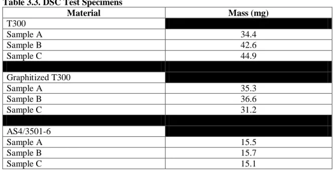
When testing a DSC sample, good thermal contact between the heat flux sensor and sample is vital for optimum results. To achieve this, the sample should lay as flush as possible with the bottom of the aluminum crucible. Each crucible is approximately 5mm in diameter and 2mm deep. Each specimen was cut into small samples with a flat surface using an uncontaminated razor blade making sure not to exceed the dimensions of the crucible. Then, each sample was weighed three times, and the average mass was documented. The mass of each test sample can be seen in Table 3.3. Each sample was placed into the crucible, and a lid was positioned on top of the crucible to fully enclose the sample. Using tweezers, the crucible was then carefully placed on the heat flux sensor making sure the crucible was centered on the sensor.
Table 3.3. DSC Test Specimens Material Mass (mg) T300 Sample A 34.4 Sample B 42.6 Sample C 44.9 Graphitized T300 Sample A 35.3 Sample B 36.6 Sample C 31.2 AS4/3501-6 Sample A 15.5 Sample B 15.7 Sample C 15.1 3.2.3 Experimental Procedure
The differential scanning calorimetry experiment was performed following testing standard ASTM E1269, Standard Test Method for Determining Specific Heat Capacity by Differential Scanning Calorimetry. The differential scanning calorimeter and data acquisition system was initialized and was allowed to reach thermal equilibrium. During this period the apparatus was purged with argon gas at a rate of 50 mL/min to produce an inert testing atmosphere. To measure the specific heat of a sample a minimum of three runs must be performed.
Before the specific heat of the carbon composites was determined a baseline and reference test were performed. Since the samples were placed inside an aluminum crucible for testing, the crucible will add a contact resistance to sample. The baseline
corrects for this contact resistance increasing the accuracy of your results. The initial baseline run was performed by placing two empty crucibles in the designated location on heat flux sensor as seen in Figure 3.7. The furnace was heated to the designated initial temperature of the program, and held there isothermally at least four minutes while the calorimeter recorded the thermal curve. The crucibles were heated to the final temperature at rate of 20°C/min and held isothermally again while the calorimeter recorded the thermal curve.
Following the baseline run, the calorimeter testing chamber was cooled to ambient temperature. The crucible on reference location in the testing chamber was replaced with a sapphire reference. After applying the previous baseline to correct for the aluminum crucible, the same temperature program used for the baseline was executed for the sapphire reference. The measured specific heat of the sapphire was compared to the known specific heat value for sapphire to determine the error. The test was repeated for the carbon composite samples. To verify that the baseline did not alter, a baseline established after every fourth test. Using the measure sapphire as a reference, the ratio method was used to determine the specific heat of the carbon composites.
CHAPTER 4
RESULTS AND DISSCUSSIONS
4.1 Thermal Diffusivity
The flash method was used to measure the thermal diffusivity in the transverse direction of the carbon composites. The thermal diffusivity of the carbon-carbon composites were measured between room temperature and 315°C. This was limited by the temperature range of the apparatus. The carbon-epoxy composite maximum temperature was reduced to 150°C due to the lower service temperature, 177°C of the epoxy. Figure 4.1 displays temperature dependence of the transverse diffusivity for AS4/3501-6.
The thermal diffusivity of the AS4/3501-6 through the temperature 20°C to 150°C ranged from 0.00375 cm2/s to 0.00461 cm2/s. The thermal diffusivity of AS4/3501-5 decrease from room temperature to 80°C. After 80°C the thermal diffusivity remained consistent throughout the remaining portion of the temperature range. Figure 4.2 displays the thermal diffusivity of the T300 carbon-carbon composite. At the initial temperature of 25°C, the thermal diffusivity was 0.0165 cm2/s. The thermal diffusivity remained very consistent throughout the temperature range until the end where a slight decrease was noticed. There, the diffusivity dropped slightly to 0.0139 cm2/s. Overall, temperature had a minimum effect on both the AS4/3501-6 carbon-epoxy and the T300 carbon-epoxy in the tested temperature ranges.
It appeared that graphitizing the carbon fibers had an effect on the thermophysical properties of the carbon composites. Unlike the other two carbon composites, the thermal diffusivity of the graphitized T300 carbon-carbon composite was very temperature dependent. The thermal diffusivity of the composite decreased from 0.143 cm2/s to 0.069 cm2/s, a 52% decline in thermal diffusivity due to temperature. This can be seen in Figure 4.3. By graphitizing the fibers, the thermal diffusivity increased by as much as 767% at room temperature and 400% above 300°C. This effect is seen in Figure 4.4.
Figure 4.4. Transverse Thermal Diffusivity Comparison of T300 Composites
According to the testing standard [16], the optimum thickness of the tested samples should be chosen so that the time to reach half of the maximum temperatures (half-time), t1/2 falls within the 10 to 1000 ms (0.01 to 1 s) range. To verify that the
samples were the proper thickness, an initial test was performed to check the half-times of the tested material. The half-times attained at each temperature during this trial were recorded. The results from the initial trial can be seen in Table 4.1. The half-time for each material fell within the acceptable range according to the testing standard verifying that the proper thickness was chosen.
Table 4.1. Half-Time of the Test Materials Material Temperature (°C) t1/2 (s) AS4/3501-6 22 0.390339255 125 0.398739398 T300 27 0.440540105 125 0.447540224 247 0.570177555 315 0.477274060 T300 2500°C 23 0.042000044 100 0.054200251 247 0.077067301 314 0.086600795
To check the validity of the results obtained during the experiment, the diffusivity must be calculated at a minimum of two other points besides the half-time on the rise curve of the thermogram [16]. Using the general form of the flash method equation for thermal diffusivity, the thermal diffusivity can be calculated at any point alone the measure thermogram:
(5.1)
where tx is the time required for the temperature to reach x percent of ΔTmax, and Kx is the
corresponding flash method diffusivity constant. The values of the constant can be found in Table 4.2.
The calculated values for the thermal diffusivity on the rise curve should all be the same when not considering heat losses. If the thermal diffusivity values at 25% and 75% of ΔTmax lie within ± 2% of the half-time thermal diffusivity value, the overall accuracy
temperature. If the thermal diffusivity values lie outside this range, a correction using Clark and Taylor’s analysis is necessary. To calculate the error between the thermal diffusivity values on the rise curve of the thermogram, the following equation was used:
(4.2) where α is the thermal diffusivity measured at the half-time of the thermogram, αn is the
thermal diffusivity at other instants on the thermogram. Table 4.3 displays the percent error calculated at 25% and 75% of the thermogram for AS4/3501-6.
Table 4.2. Constant kx for Various Percent Rises [16]
x (%) Kx 10.00 0.066108 20.00 0.084251 25.00 0.092725 30.00 0.101213 33.33 0.106976 40.00 0.118960 50.00 … 60.00 0.162236 66.67 0.181067 70.00 0.191874 75.00 0.210493 80.00 0.233200 90.00 0.303520 … …
Examining two flashes performed on AS4/3501-6, the percent error at 25% and 75% of ΔTmax was within the ± 2% range during a flash at 22°C. Looking at the percent
percent error of the carbon-carbon composites are displayed in the following Tables 4.4 and 4.5. When examining the percent error of thermal diffusivity for the carbon-carbon composites, the percent error was outside of the 2% threshold but still acceptable. Clark and Taylor correction was applied to compensate for the error.
Table 4.3. Thermal Diffusivity Validation of AS4/3501-6 Composite
Temperature °C x(%) Diffusivity cm2/s % Error
22 25 0.004617 0.45 50 0.004597 75 0.004648 1.11 125 25 0.004158 3.04 50 0.004289 75 0.004531 5.64
Table 4.4. Thermal Diffusivity Validation of T300 Composite
Temperature °C x(%) Diffusivity cm2/s % Error
27 25 0.017618 4.28% 50 0.018405 75 0.019660 6.82% 125 25 0.016334 2.40% 50 0.016735 75 0.017511 4.64% 247 25 0.013759 4.51% 50 0.014409 75 0.015144 5.10% 315 25 0.015386 1.95% 50 0.015692 75 0.016391 4.45%
Table 4.5. Thermal Diffusivity Validation of Graphitized T300 Composite
Temperature °C x(%) Diffusivity cm2/s % Error
23 25 0.150846 1.89% 50 0.153748 75 0.160724 4.54% 100 25 0.116599 2.13% 50 0.119140 75 0.123136 3.35% 247 25 0.082122 1.99% 50 0.083789 75 0.086718 3.50% 314 25 0.070874 1.60% 50 0.072029 75 0.074412 3.31%
Visual analysis can be done by plotting the normalized thermogram of a flash pulse against a theoretical model of the thermogram that assumes no losses. By plotting the normalized thermograms against the theoretical model, one can observe radiation loses and finite pulse time effect. Overshooting of the theoretical model by the experimental data verifies there was a finite pulse time effect during the shot. In addition, if the experimental data falls below the theoretical model then radiation losses were present during that flash pulse. Clark and Taylor’s correction factor accounts for these losses and adjusts the thermal diffusivity as necessary. Figures 4.5, 4.6, and 4.7 display multiple thermograms at various temperatures of the tested carbon composites.
Figure 4.5. Comparison of the AS4/3501-6 Composite Thermograms to the Theoretical Model
Figure 4.6. Comparison of the T300 Composite Thermogram to the Theoretical Model
Figure 4.7. Comparison of the Graphitized T300 Composite to the Theoretical Model
Visually examining the thermograms of the tested carbon composites, the graphitized T300 carbon-carbon composite normalized thermograms were very consistent with the theoretical model. This symbolized that the radiation heat losses were minimum during the flash pulse. Unlike the graphitized T300 carbon-carbon composites, noticeable losses due to radiation heat losses were noticed for the T300 carbon-carbon composite and the AS4/3501-6 carbon-epoxy composites after the peak change of temperature was achieved. This reflects the fact that a correction was need.
In addition to the numerical validation, the AS4/3501-6 and graphitized T300 carbon composites were tested at Oak Ridge National Laboratory on their FlashLine™ 5000 laser flash apparatus. The experiment was performed using the same sample
apparatus were compared to the results obtained using the FlashLine™ 2000 xenon flash. A comparison of the results can be seen in Figures 4.8 and 4.9.
Comparing the test results of laser flash apparatus and the xenon flash for the AS4/3501-6 carbon epoxy composites, the diffusivity values were within 3.8% of each other and overlapping in some portions of the data set. Similarly, the thermal diffusivity values obtained from the graphitized T300 carbon-carbon composite were within 7%. In addition, the carbon composites followed the same trend with both apparatus verifying the accuracy and reproducibility of the results.
Figure 4.9. Graphitized T300 Composite Thermal Diffusivity Comparison
4.2 Specific Heat
To confirm that the user-induced error of the differential scanning calorimeter was insignificant, the specific heat of the reference sapphire was tested before and after the carbon composites were tested. The heating curve was analyzed using the ratio method. The experimental result was compared with the known value for the reference to estimate the error induced by the user. Figure 4.10 displays the results from the comparison. A maximum error of 1.45% was observed during the preliminary and post runs. Next, the specific heat of the carbon composite samples was tested. The result can be seen in Figures 4.11, 4.12, and 4.13.
Figure 4.10. Specific Heat of the Sapphire Reference
Figure 4.12. Specific Heat of the T300 Composite
The carbon-carbon and carbon-epoxy composites followed the characteristic specific heat trend with increasing temperature. Unlike the thermal diffusivity results from the flash method, the heat treatment of the fiber appeared not to have an effect of the carbon composite’s ability to store energy. The specific heat of the AS4/3501-6 carbon-epoxy composite increased from 1 J/g°C to 1.3 J/g°C. The specific heat of the T300 and graphitized T300 carbon-carbon composites were consistent; increasing from approximately 0.8 J/g°C to 1.8 J/g°C. From the initial temperature until approximately 400°C, the difference between the specific heat values was not greater than 3%. By the end of the temperature range, less than a 6% difference was noted. A comparison of the T300 carbon-carbon composites can be seen in Figure 4.14.
4.3 Thermal Conductivity
Using the density, specific heat, and thermal diffusivity in the transverse direction, the thermal conductivity in the transverse direction of the composites was determined using the following relationship,
(4.2)
The calculated thermal conductivity values for the carbon composites can be seen in Figures 4.15, 4.16, and 4.17. In addition, the thermal conductivity of the T300 and graphitized T300 carbon-carbon composites can be seen in Figure 4.18.
Figure 4.16. Thermal Conductivity of the T300 Composite
Figure 4.18. Thermal Conductivity Comparison of Carbon-Carbon Composites
The thermal conductivity of the AS4/3501-6 carbon-epoxy composite ranged from approximately 0.6 W/mK to 0.7 W/mK over the temperature range. The effect of heat treating the T300 carbon fibers was also noticed in the thermal conductivity results. The thermal conductivity of the T300 carbon-carbon composite was found to range from approximately 2 W/mK to 3 W/mK increasing with temperature similar to AS4/3501-6 carbon-epoxy composite. Temperature appeared to have very little effect on the graphitized T300 carbon-carbon composite’s thermal conductivity in the measurement temperature range. The thermal conductivity remained consistent at approximately 15 W/mk. Table 4.6 summarizes the results of the thermophysical properties.
Table 4.6. Summary of Thermophysical Properties
Thermal Properties AS4/3501-6 T300 Graphitized T300
Thermal Diffusivity (cm2/s) 0.0037 - 0.0046 0.0139 -0.0165 0.0690 – 0.1430 Specific Heat (J/g°C) 1.0 - 1.3 0.8 – 1.8 0.8 – 1.8 Thermal Conductivity (W/mK) 0.6 – 0.7 2.0 – 3.0 15
CHAPTER 5 CONCLUSION
In this research, the thermal properties of carbon-carbon composites produced by the resin transfer molding process and the unidirectional, continuous carbon-epoxy laminate, AS4/3501-6 were determined. The carbon-carbon composites consisted of graphitized and non-graphitized T300 PAN based carbon fiber and PT-30 cyanate ester resin. Using the flash method, the thermal diffusivity in the transverse direction of the carbon composites was measured. Analysis was performed to validate the accuracy of the thermal diffusivity results. In addition, the thermal diffusivity was measured at Oak Ridge National Laboratory (ORNL) using their laser flash apparatus. The thermal diffusivity determined at North Carolina A&T State University using the xenon flash apparatus were in good agreement with those obtained at ORNL.
A differential scanning calorimeter was used to measure the specific heat of the carbon composites. The specific heat of the reference material, sapphire was measured and compared to the known values of sapphire to verify that the user induced error was trivial. The specific heat of the carbon composites was determined using the heating curve of the differential scanning calorimeter. Ultimately, the thermal conductivity in the transverse direction was determined using the density, specific heat, and thermal diffusivity in the transverse direction of the carbon composites.
Upon completion of this research several recommendations for future work were made.
1. Measure the thermal diffusivity, specific heat, and conductivity in the in-plane direction of the carbon composites and confirm if there are any directional effects of the thermophysical properties.
2. Measure the thermal diffusivity, specific heat, and conductivity of the individual components of the carbon composites separately, and attempt to predict the thermophysical properties of the entire composite from these.
3. Measure the thermal diffusivity, specific heat, and conductivity of the composites while varying fiber volume of the composites, and validate the effects of the fiber content of the composites.
REFERENCES
[1] Daniel, I. M., and Ishai, O., 2006, Engineering Mechanics of Composite Materials, Oxford University Press, Inc., New York
[2] Cernuschi, F., Bison, P. G., Marinetti, S., Figari, A., Lorenzoni, L., E., and Grinzato, E., 2000, “Comparison of Thermal Diffusivity Measurement Techniques”
[3] Center of Composite Research http://www.ncat.edu/~ccmradm/ccmr/
[4] Çengel, Y. A., 1998, Heat Transfer, A Practical Approach, McGraw-Hill Companies, Inc, Boston
[5] Rolle, K. C., 2000, Heat and Mass Transfer, Prentice Hall, New Jersey
[6] Incropera, F. P., and DeWitt, D. P., 1996, Fundamentals of Heat and Mass Transfer, John Wiley & Sons, New York
[7] Salazar A., 2003, “On Thermal Diffusivity,” European Journal of Physics, Vol. 24, pp. 351–358.
[8] Bentur A., and Mindess S., 2007, Fibre Reinforced Cementitious Composites, Taylor and Francis, New York
[9] Parrott J. E., and Stuckes A. D., 1975, Thermal Conductivity of Solids, Pion Limited, London
[10] Abalim, F., Shivakumar, K., Hamidi, N., and Sadler, R., 2002, “An RTM Densification Method of Manufacturing Carbon-Carbon Composites Using Primaset PT-30 Resin,” Pergamon, Carbon 41 pp893-901.
[11] Hexcel, Magnamite® AS4 Carbon Fiber Product Data, www.hexcel.com
[12] Tritt, T., 2004, Thermal Conductivity: Theory, Properties, and Applications, Plenum Publishers, New York
[13] Psaras, P. A., and Langford, H. D., 1987, Advancing Materials Research, The National Academies Press, Washington, D.C.
[14] Committee on Materials Science and Engineering, 1989, Materials Science and Engineering for the 1990s: Maintaining Competitiveness in the Age of Materials, The National Academies Press, Washington, D.C., p176
[15] Parker, W. J., Jenkins, R. J., Butler, C. P., and Abbott, G. L., 1979, “Flash Method of Determining Thermal Diffusivity Heat Capacity and Thermal Conductivity,” J. Appl. Phys., 32, Vol 9
[16] ASTM Standard E1461, 2007, “Standard Test Method for Thermal Diffusivity by the Flash Method,” ASTM International, West Conshohocken, PA, http://www.astm.org
[17] Carslaw H. S., and Jaeger J. C., 1959, Conduction of Heat in Solids, Oxford University Press, New York
[18] NETZSCH, “System Features Operating Instructions Micro-Flash-Apparatus,” LFA 457.
[19] Cowan, R. D., 1962, “Pulse Method of Measuring Thermal Diffusivity at High Temperatures,” Journal of Applied Physics V34 #4, pp926-927
[20] Clark, L. M., and Taylor R. E., 1975, “Radiation Loss in the Flash Method for Thermal Diffusivity,” Journal of Applied Physics, Vol. 46, No.2
[21] Anter, “FlashLine™ Thermal Diffusivity Measuring System Operation and Maintenance Manual Part 1 Flashline 2000”
[22] Höhne, G., Hemminger, W. F., and Flammersheim, H. J., 2003, Differential Scanning Calorimetry, Springer, Germany pg. 1
[23] ASTM Standard E1269, 2005, “Standard Test Method for Determining Specific Heat Capacity by Differential Scanning Calorimetry,” ASTM International, West Conshohocken, PA, http://www.astm.org
[24] Çengel, Y. A., 2002, Thermodynamics, An Engineering Approach, McGraw-Hill Companies, Inc, Boston
[25] NETZSCH, 2008, “Technical Data Sheet DSC 200 F3 Maia” [26] NETZSCH, 2008, “Operating Instructions DSC 200 F3 Maia”
APPENDIX
THE FLASH METHOD EQUATION DERIVATION
The following is a complete derivation of the flash method’s thermal diffusivity equation.
Starting with Carslaw and Jeager’s [17] equation of temperature distribution within a thermally insulated solid of uniform thickness L, Parker et al. [15] derived the
mathematical expression to calculate thermal diffusivity:
L n L dx L x n x T L x n L t n L dx x T L t x T 0 1 0 2 2 2 cos ) 0 , ( cos exp 2 ) 0 , ( 1 ) , ( (1)where α is the thermal diffusivity of the material. If a pulse of radiant energy Q is instantaneously and uniformly adsorbed in the small depth g at the front surface x = 0, the
temperature distribution at that instant is given by the following: for 0 < x < g and, g C Q x T ) 0 , ( (2) for g < x < L. T(x,0) = 0 (3) *∫ ∫ + ∑ ( ) *∫ ∫ + (4)
dx dx L x n g C Q L x n L t n L dx dx g C Q L t x T L g g n L g g 0 cos cos exp 2 0 1 ) , ( 0 1 2 2 2 0 (5)
g n g n L L x n g C Q L x n L t n L x L g C Q t x T 0 1 2 2 2 0 sin cos exp 2 ) , (
(6) [ ] ∑ ( ) [ ( ) ( ) ] (7)
n L L g n g C Q L x n L t n L L g C g Q t x T n sin cos exp 2 ) , ( 1 2 2 2 (8) �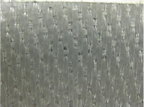

![Figure 3.3. Thermogram Displaying the Half-Time [18]](https://thumb-us.123doks.com/thumbv2/123dok_us/110547.2512570/32.918.258.717.158.436/figure-thermogram-displaying-the-half-time.webp)


![Figure 3.6. Cross Section View DSC 200 F3 Maia® [26]](https://thumb-us.123doks.com/thumbv2/123dok_us/110547.2512570/43.918.163.815.160.557/figure-cross-section-view-dsc-f-maia.webp)