Risk Management with Basis Risk
byJingong Zhang
A thesis
presented to the University of Waterloo in fulfillment of the
thesis requirement for the degree of Doctor of Philosophy
in
Actuarial Science
Waterloo, Ontario, Canada, 2018
c
Examining Committee Membership
The following served on the Examining Committee for this thesis. The decision of the Examining Committee is by majority vote.
External Examiner: Rogemar S. Mamon
Professor, Department of Statistical and Actuarial Sciences, Western University
Supervisor(s): Ken Seng Tan
Professor, Department of Statistics and Actuarial Science, University of Waterloo
Chengguo Weng
Associate Professor, Department of Statistics and Actuarial Science, University of Waterloo
Internal Member(s): Adam Kolkiewicz
Associate Professor, Department of Statistics and Actuarial Science, University of Waterloo
Alexander Schied
Professor, Department of Statistics and Actuarial Science, University of Waterloo
Internal-External Member: Peter A. Forsyth
Distinguished Professor Emeritus, Cheriton School of Computer Science, University of Waterloo
I hereby declare that I am the sole author of this thesis. This is a true copy of the thesis, including any required final revisions, as accepted by my examiners.
I understand that my thesis may be made electronically available to the public.
Abstract
Basis risk occurs naturally in a variety of financial and actuarial applications, and it introduces additional complexity to the risk management problems. Current literature on quantifying and managing basis risk is still quite limited, and one class of important questions that remains open is how to conduct effective risk mitigation when basis risk is involved and perfect hedging is either impossible or too expensive. The theme of this thesis is to study risk management problems in the presence of basis risk under three settings: 1) hedging equity-linked financial derivatives; 2) hedging longevity risk; and 3) index insurance design.
First we consider the problem of hedging a vanilla European option using a liquidly traded asset which is not the underlying asset but correlates to the underlying and we investigate an op-timal construction of hedging portfolio involving such an asset. The mean-variance criterion is adopted to evaluate the hedging performance, and a subgame Nash equilibrium is used to define the optimal solution. The problem is solved by resorting to a dynamic programming procedure and a change-of-measure technique. A closed-form optimal control process is obtained under a general diffusion model. The solution we obtain is highly tractable and to the best of our knowl-edge, this is the first time the analytical solution exists for dynamic hedging of general vanilla European options with basis risk under the mean-variance criterion. Examples on hedging Eu-ropean call options are presented to foster the feasibility and importance of our optimal hedging strategy in the presence of basis risk.
We then explore the problem of optimal dynamic longevity hedge. From a pension plan sponsor’s perspective, we study dynamic hedging strategies for longevity risk using standardized securities in a discrete-time setting. The hedging securities are linked to a population which may differ from the underlying population of the pension plan, and thus basis risk arises. Drawing from the technique of dynamic programming, we develop a framework which allows us to obtain analytical optimal dynamic hedging strategies to achieve the minimum variance of hedging error. For the first time in the literature, analytical optimal solutions are obtained for such a hedging problem. The most striking advantage of the method lies in its flexibility. While q-forwards are considered in the specific implementation in the paper, our method is readily applicable to other securities such as longevity swaps. Further, our method is implementable for a variety of
longevity models including Lee-Carter, Cairns-Blake-Dowd (CBD) and their variants. Extensive numerical experiments show that our hedging method significantly outperforms the standard “delta” hedging strategy which is commonly adopted in the literature.
Lastly we study the problem of optimal index insurance design under an expected utility maximization framework. For general utility functions, we formally prove the existence and uniqueness of optimal contract, and develop an effective numerical procedure to calculate the optimal solution. For exponential utility and quadratic utility functions, we obtain analytical ex-pression of the optimal indemnity function. Our results show that the indemnity can be a highly non-linear and even non-monotonic function of the index variable in order to align with the actu-arial loss variable so as to achieve the best reduction in basis risk. Due to the generality of model setup, our proposed method is readily applicable to a variety of insurance applications including index-linked mortality securities, weather index agriculture insurance and index-based catastro-phe insurance. Our method is illustrated by a numerical example where weather index insurance is designed for protection against the adverse rice yield using temperature and precipitation as the underlying indices. Numerical results show that our optimal index insurance significantly outperforms linear-type index insurance contracts in terms of reducing basis risk.
Acknowledgements
I would like to express my deepest gratitude to my supervisors, Professor Ken Seng Tan and Professor Chengguo Weng. Their profound knowledge, cautious attitude, inspiring guidance and continuous support turn me from a rookie who barely knew where to start into a self-proclaimed independent researcher. The freedom I am given to follow my research curiosity and interests makes the beginning of my academic career so colorful and enjoyable.
I would also like to thank all the committee members: Professor Adam Kolkiewicz, Professor Alexander Schied, Professor Peter Forsyth and Professor Rogemar Mamon for all those insight-ful suggestions and comments, which lead to significant improvements in both the content and the presentation of this thesis.
I acknowledge financial support from the Department of Statistics and Actuarial Science, University of Waterloo, and the Society of Actuaries Hickman Scholarship, which helps me a lot to relieve my financial stress and better focus on my research during my study life.
My friends and classmates also provide me lots of contributory ideas and opinions during my research process, and I truly appreciate all the help.
Finally, thank you to my parents and family for giving me unconditional support, without which this thesis would not even be possible in the first place. Special thanks to my wife Wenjun: meeting you is the most beautiful thing that happens in Waterloo and in my life.
Dedication
Table of Contents
List of Tables xii
List of Figures xiii
1 Introduction 1
1.1 Background . . . 1
1.2 Objectives and outline . . . 5
2 Optimal Hedging with Basis Risk under Mean-Variance Criterion 7 2.1 Introduction . . . 7
2.2 Formulation of the optimal hedging problem . . . 11
2.3 Optimal time consistent hedging strategy. . . 16
2.3.1 The extended HJB equation . . . 17
2.3.2 Verification theorem . . . 18
2.3.3 Equilibrium solution . . . 21
2.4 Discussions . . . 29
2.4.1 The case with no basis risk . . . 30
2.4.3 The limiting case whenγ → ∞with no basis risk . . . 32
2.4.4 Solutions under geometric Brownian motions . . . 34
2.5 Numerical examples . . . 39
2.6 Conclusion . . . 43
3 Optimal Dynamic Longevity Hedge with Basis Risk 44 3.1 Introduction . . . 44
3.2 Problem setup . . . 47
3.2.1 Stochastic mortality model . . . 47
3.2.2 Pension liability . . . 48
3.2.3 Dynamic hedge with q-forward . . . 49
3.2.4 Hedging objective . . . 52
3.3 Derivation of the optimal solution . . . 55
3.3.1 The Bellman equation . . . 55
3.3.2 Solution of the Bellman equation . . . 57
3.4 Hedging Canadian mortality rates with UK mortality rates . . . 60
3.4.1 Data and assumptions . . . 61
3.4.2 Approximation to forward mortality rates . . . 62
3.4.3 Benchmark method . . . 63
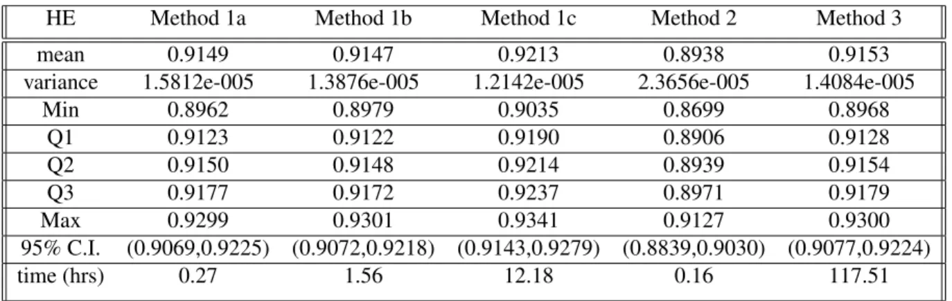
3.4.4 Baseline result . . . 64
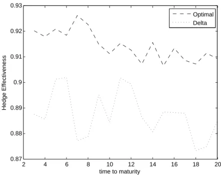
3.4.5 Robustness to q-forwards’ time to maturity . . . 66
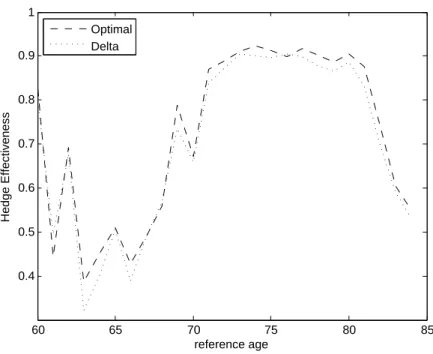
3.4.6 Robustness to q-forwards’ reference age . . . 68
3.4.7 Robustness to model risk . . . 69
4 Index Insurance Design 75
4.1 Introduction . . . 75
4.2 Problem Setup. . . 79
4.3 Existence and Uniqueness of the Optimal Design . . . 81
4.3.1 Uniqueness of the optimal solution . . . 81
4.3.2 Existence of optimal solution . . . 82
4.4 Computing the Optimal Solution . . . 87
4.4.1 The ODE method . . . 88
4.4.2 Quadratic utility . . . 92
4.4.3 Exponential utility . . . 94
4.5 Applications in Weather Index Insurance Design. . . 95
4.5.1 Dependence modeling . . . 96
4.5.2 Quadratic utility . . . 97
4.5.3 Exponential utility . . . 101
4.5.4 Logarithmic utility . . . 102
4.5.5 Comparison with linear contracts . . . 103
4.5.6 An example of bivariate-index insurance. . . 105
4.6 Conclusion . . . 108
5 Conclusion and Future Research 109
References 112
A Appendix for Chapter 2 121
A.1 Proof of Proposition 2.1. . . 121
A.2 Equilibrium value function for futures contract . . . 125
A.3 Equilibrium value function for European call options . . . 126
B Appendix for Chapter 3 127
B.1 Approximations for forward survival rates in Section 3.4.2 . . . 127
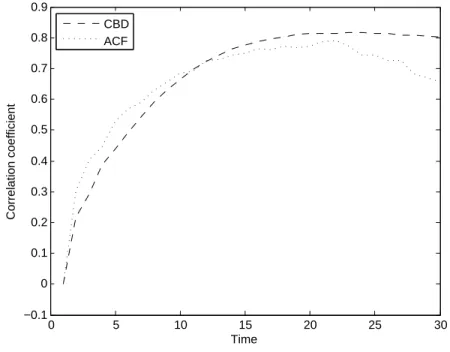
B.2 Approximations for forward survival rates under CBD model in Section 3.4.7 . . 128
C Appendix for Chapter 4 131
List of Tables
2.1 Parameter values for the hedging examples. . . 39
2.2 Comparison of different strategies on hedging European call option (γ = 1) . . . 41
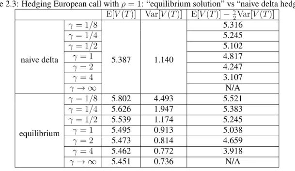
2.3 Hedging European call with ρ = 1: “equilibrium solution” vs “naive delta hedge”. . . 42
2.4 Hedging European call with ρ = 0.9: “equilibrium solution” vs “naive delta hedge”. . . 42
3.1 Results of Five Experiments . . . 65
List of Figures
3.1 HE with different time to maturity . . . 67
3.2 HE with different reference ages . . . 69
3.3 Change with time to maturity . . . 73
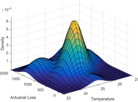
4.1 Joint densityf(x, y)of the actual loss and the average temperature. . . 96
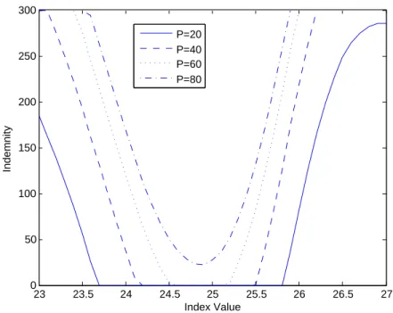
4.2 Optimal indemnity functions for different premium levels. . . 98
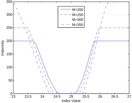
4.3 Optimal indemnity for different maximum indemnity levels. . . 99
4.4 Basis risk (i.e., the standard deviation of residual risk) for different levels of premium and maximum indemnity. . . 100
4.5 Optimal indemnity under exponential utility. . . 101
4.6 Optimal indemnity under logarithmic utility. . . 103
4.7 Comparison of optimal indemnity functions under three different utilities. . . 104
4.8 Effectiveness: our optimal index insurance vs. the linear-type contract. . . 105
4.9 Indemnity function of a bivariate-index insurance: temperature and precipitation. 106 4.10 Effectiveness improvement of additional index. Basis risk is measured by stan-dard deviation of residual risk. . . 107
Chapter 1
Introduction
1.1
Background
Broadly speaking, basis risk is defined as the non-hedgeable portion of risk as attributed to the imperfect correlation between the asset to be hedged and the asset used for hedging. It implies that the hedging will be imperfect and the hedged position still carries some residual risk. The existence of basis risk introduces additional complication for risk management, and it may have detrimental effects when it is overlooked. Therefore it is important for risk managers to pay attention to the identification, assessment, and management of basis risk.
Basis risk naturally occurs in a variety of financial and actuarial problems. A typical example in the financial market is that the hedging for a derivative written on a non-tradable asset is often conducted via trading over one liquidly traded asset which is closely correlated with the non-tradable underlying asset. A relevant concept is finance and economics is the incomplete market in which the number of Arrow-Debreu securities is less than the number of states of nature, and thus some payoffs in the market cannot be replicated by tradable securities in that market. In this case, the hedger would normally aim at designing a hedging scheme with other tradable assets to minimize the negative impact resulted from the mismatch between these assets and therefore achieve certain financial objectives.
The second example where basis risk plays a critical role is longevity risk management. In recent decades longevity risk has become one of the most dominant risks, particularly for pension plan sponsors and annuities providers. Longevity risk is any risk associated with the unpredicted increasing life expectancy, and it will eventually translate into higher than expected payout ratios for pension plans and insurance companies. Hedging of longevity risk is an important problem because the risk is non-diversifiable. As such some longevity securities such as longevity bonds and longevity swaps have been issued in an attempt to address longevity risk. However, these longevity securities have payoffs that are linked to some standardized populations while the pension plan sponsors and annuity providers are more concerned with the longevity experience underlying the pensioners and annuitants. These experiences are not perfectly related to the experience of the standardized population underlies the longevity securities and hence population basis risk arises. Li and Hardy (2011) give an empirical example to hedge a pension plan on the female Canadian population with a longevity index on the U.S. population. When measured by Value-at-Risk, the magnitude of reduction in basis risk can be as high as 10.14%.
Another area where basis risk is prevalent is the agricultural index insurance where the basis risk is cited as a primary concern in agricultural risk management (Brockett et al., 2005). Index insurance is an innovative approach to insurance provision which pays indemnity determined by certain relevant indices rather than the actual losses experienced by policyholders, and a typical example of using index insurance is in the area of agricultural insurance. Agricultural production is very vulnerable to weather risks and hence providing insurance protection to farmers is im-portant. Traditionally agricultural insurance is indemnity based, i.e. farmers will be reimbursed based on the incurred losses. This product, however, is known to generate moral hazard with high underwriting cost, especially offering to regions with numerous small farms. Alternatively, weather index insurance is gaining popularity to hedge against agricultural production loss. Plau-sible indices include temperature, precipitation, sunshine as well as those remote sensing indices based on satellites images such as the Normalized Difference Vegetation Index (NVDI). In this context, farmers are similarly exposed to basis risk due to the imperfect correlation between the weather index and the crop yield.
This thesis focuses on three risk management problems, and the evolving theme in these applications is the basis risk that is present in derivative hedging, longevity risk hedging and
agricultural index insurance. It should be noted that there are other interesting risk management problems involving basis risk. Some notable examples include hedging of equity-linked insur-ance products such as variable annuities (Ng and Li, 2013) and catastrophic risk management (Doherty, 1997; Li and Yu, 2002; Cummins et al., 2004).
Basis risk generally comes from the mismatch between the hedging objective and the hedging instrument. More specifically, this mismatch may come in different forms and typical examples include: 1) hedging objective and hedging instrument are totally different type of assets, e.g., one is agricultural production and the other is a weather index; 2) hedging objective and hedging instrument are the same type but with different underlying assets, time to maturity and so on; 3) hedging objective and hedging instrument are based on exactly the same asset, but the way to construct the hedging portfolio makes the hedging imperfect due to budge constraint, trading fre-quency, and etc. Mathematically, we usually define this mismatch between the hedging objective and the hedging instrument by assuming that two random variables are not equal almost surely1
in static settings, or two stochastic processes are not indistinguishable2 in dynamic settings.
The study of basis risk contains two major aspects: 1) how to model the dependence struc-ture between two random variables or stochastic processes and how to measure the difference between them in order to quantify basis risk; 2) based on a given dependence structure between the hedging objective and the hedging instrument, how to construct a hedging portfolio or a risk mitigation strategy in order to achieve the hedger’s certain financial objective. The former, the modeling problem, itself is a very broad area, and under each specific setting the way to model the dependence structure can be very different. For example, in the literature of longevity risk, one common way to model the dependence between multiple populations is to introduce an addi-tional common factor to represent their co-movement into the original model (such as Lee Carter model, Cairns-Blake-Dowd (CBD) model and etc.). This is quite different from those commonly used dependence modeling techniques such as copulas, and is not that commonly used in the other contexts of risk management. In this thesis we focus on the second aspect, and explic-itly exploit the current existing models as our starting point. In other words, we study these
1Two random variablesXandY are defined as equal almost surely if
P(X =Y) = 1.
2Two stochastic processes {X
t}t≥0 and {Yt}t≥0 are defined to be indistinguishable if P(ω : X(t, ω) =
risk management problems in the presence of basis risk by assuming the underlying models and dependence structures are given exogenously.
In the mathematical finance literature, there are many papers that discuss the problem of hedging contingent payoffs in an incomplete market setting. Since the contingent claim of interest cannot generally be replicated by any hedging strategies which are self-financing and perfectly match the target payoff function at the same time, there are two major approaches of constructing the hedge: first, the hedger may relax the self-financing constraint imposed on the hedging strategy by continuously injecting money into the hedging plan, and only re-quires it to perfectly match the payoff function of the contingent claim to be hedged; second, the hedger still sticks to self-financing hedging plans and thrives to minimize the “distance” be-tween the hedging objective and the hedging portfolio. The first method was studied by F¨ollmer and Schweizer (1991) and Schweizer (1999), and they introduced the concept of locally risk-minimizing strategy to minimize the expected cumulative cost under a quadratic criterion, and obtained the hedging strategy through the F¨ollmer-Schweizer decomposition. Some further re-search was conducted by Møller (1998, 2001) with applications for hedging insurance payoffs such as unit-linked life insurance contracts. The second method was discussed by Duffie and Richardson (1991) under the mean-variance criterion, and by Davis (2006) and Musiela and Zariphopoulou (2004) under an exponential utility maximization framework.
In the insurance and actuarial science literature, although there are articles addressing basis risk for various risk management problems, such as longevity hedge with standardized mortality-linked securities (Li and Hardy, 2011; Coughlan et al., 2011; Cairns, 2013; Zhou and Li, 2016), agricultural production protection with weather derivatives and weather insurance (Woodard and Garcia, 2008; Brockett et al., 2005; Chantarat et al., 2007; Jensen, et al., 2016) and catastrophe risk mitigation by catastrophe securities (Lee and Yu, 2002; Cummins et al., 2004), most of them are empirical studies concentrating on very specific applications.
1.2
Objectives and outline
The thesis aims at developing innovative methodologies by focusing on three risk management problems in the presence of basis risk, namely, financial derivative hedging, longevity risk hedg-ing and index insurance design, in three separate chapters. Each chapter begins with formulathedg-ing the problem in an optimization framework, proceeds with mathematical derivation to solve the optimization problem, and finishes with numerical examples showing the applicability and supe-riority of our proposed solutions. The rest of this thesis is organized as follows.
Chapter2studies the hedging problem for general European-style financial derivatives whose underlying assets are not traded in the market. Therefore we use another correlated and liquidly traded asset as the hedging instrument. We adopt the mean-variance criterion to evaluate the hedging performance, and use a subgame Nash equilibrium to define the optimal solution to overcome the “time-inconsistent” issue which arises inherently from the mean-variance crite-rion. The problem is solved by resorting to a dynamic programming procedure and a change-of-measure technique. Numerical examples for hedging futures and European call options are presented to showcase the performance of our proposed optimal strategy.
Chapter 3 investigates the problem of longevity hedge using standardized longevity secu-rities. We study dynamic hedging strategies for longevity risk from a pension plan sponsor’s perspective in a discrete-time setting. Our assumptions about the underlying stochastic mortality models are quite general so that our results can be applied to those most popularly used longevity models such as Lee-Carter, Cairns-Blake-Dowd (CBD) and their variants. The hedging instru-ments are q-forward contracts that are linked to a population different from the pension plan’s underlying population, so basis risk arises due to such a population mismatch. We apply the dynamic programming technique to develop a framework which allows us to obtain analytical optimal dynamic hedging strategies to achieve the minimum variance of hedging error. Exten-sive numerical experiments show that our hedging method significantly outperforms the dynamic “delta” hedging strategy which is commonly adopted in the literature.
Chapter4studies the problem of index insurance design and its applications in agricultural weather index insurance. The goal is to design an optimal index insurance contract which
max-imizes the expected utility of policyholders. For a general strictly concave utility function, the optimal solution is characterized by an implicit ordinary differential equation (ODE) problem. Our results show that the optimal indemnity can be a highly non-linear and even non-monotonic function of the index variable in order to align with the actual loss variable so as to achieve the best reduction in basis risk. Our theoretical results are illustrated by a numerical example where weather index insurance is designed for protection against the adverse rice yield using temperature and precipitation as the underlying indices. Numerical results show that our optimal index insurance significantly outperforms those linear-type index insurance contracts, which are commonly adopted in the literature and insurance practice, in terms of reducing basis risk.
Chapter5concludes the thesis and discusses some potential future works. Some additional information complementing each chapter is collected in appendices.
Chapter 2
Optimal Hedging with Basis Risk under
Mean-Variance Criterion
2.1
Introduction
It is well-known in the financial theory that when an option is written on an asset that is tradable, it can be hedged by trading in the underlying asset. What if an option is written on an asset that is either illiquid or even non-tradable? In this case, a common hedging practice is to use another asset that is tradable, highly liquid, and also has the desirable property of being highly correlated to the underlying asset of the option. Because the hedged asset does not perfectly capture the behavior of the underlying asset, there is a mismatch between the risk exposure of the hedged portfolio and the option in question; this gives rise to the so-called basis risk. As shown in Davis (2006), the basis risk could be huge even though both assets have very high correlation. This implies that the basis risk can have a detrimental effect on the hedging performance and hence it needs to be prudently managed.
Basis risk does not just confine to hedging financial derivatives, it exists in many other set-tings, notably when an index-based security is used for hedging. For example, a pension plan sponsor may choose to hedge the plan’s longevity risk by resorting to standard longevity instru-ment that is traded in the capital market. While such “standard” instruinstru-ment provides liquidity
and transparency, its payoffs are typically determined by mortality indices based on one or more populations. As the longevity experience of the pension plan can deviate significantly from the reference populations, the basis risk, or more specifically, the population basis risk, is said to occur; see also Li and Hardy (2011), Coughlan et al. (2012). Another example is in the context of managing agricultural risk. In this application, using weather derivatives for hedging agricul-tural risk could give rise to variable basis risk and spatial basis risk (e.g., Brockett et al., 2005; Woodard and Garcia, 2008). Another situation for which basis risk arises is when a farmer pur-chases a crop insurance that is based on area yield, instead of individual yield. The area-yield crop insurance, which is known as the Group Risk Plan in the U.S., is an insurance scheme with indemnity depending on the aggregated county yields. The individual-yield crop insurance, which is known as the Annual Production History Insurance in the U.S., is another insurance scheme with payoff that is linked to individual farm yields. The discrepancy between yields at the county level and at the individual level gives rise to the basis risk; see for example Skees, et al. (1997) and Turvey and Islam (1995).
A typical example in the financial market is that the hedging for an option written on a non-tradable asset is often conducted via trading over one liquidly traded asset which is closely correlated with the non-tradable underlying asset. However, one should be very careful to use such a strategy since “close correlation” between the two underlying assets cannot guarantee the hedging performance to be as good as one may desire. Indeed, Davis (2006) showed that the unhedgeable noise, which is attributed to the mismatch between the two assets, may be huge even though the two underlying assets have very high correlation, and the “naive” hedging strategy may be ineffective.
In the existing literature, analytical results on optimal hedging in the presence of basis risk can broadly be classified into two streams. In order to ensure the model’s tractability, the first stream of investigation considers hedging general derivatives with basis risk under an exponential utility maximization framework. The pioneering closed-form optimal hedging strategies were obtained by Davis (2006).1 The basic model of Davis (2006) was subsequently extended by Monoyios (2004) and Musiala and Zariphopoulou (2004) in a few interesting directions including indifference pricing, perturbation expansions, etc. All of these generalizations are restricted to
an exponential preference optimization framework. If we were to consider other optimization hedging frameworks such as under a mean-variance criterion, analytical optimal strategies with basis risk have been obtained but only for hedging futures. We classify this line of inquiry as the second stream. The main contribution is attributed to Duffie and Richardson (1991) who obtained the optimal continuous-time futures hedging policy under geometric Brownian motion assumptions. They demonstrated that the optimal hedging strategy can be derived from the normal equations for orthogonal projection in a Hilbert space. Their method, however, is not readily applicable to more general derivatives other than the futures contract. This is because their proposed method depends highly on the specific formulation of the problem and the trivial structure of the payoff function of the futures contract.
Motivated by the above two streams of investigation, this chapter attempts to address each of their limitations by studying the dynamic hedging of general European options with basis risk under a variance criterion. Since the seminal work of Markowitz (1952), the mean-variance criterion has been widely applied in finance. A key advantage of the mean-mean-variance criterion over a utility maximization objective is that in practice it is typically challenging to accurately evaluate a hedger’s utility function while the mean-variance criterion provides a sub-jective measure. Furthermore, by comparing to the expected utility approach, MacLean et al. (2011) concluded that, for less volatile financial market, the mean-variance criterion yields a better investment portfolio return.
It is important to emphasize that the optimal portfolio model of Markowitz (1952) is a one-period model. If we are interested in a dynamic portfolio selection strategy, it is important to distinguish optimal strategy that is “pre-commitment” from “time-consistent planning” because of the added possibility of re-optimizing and re-balancing the portfolio at intertemporal times. After a decision maker obtained his/her optimal dynamic strategy at timet1, the decision maker
might find that the adopted strategy fromt1 does not necessarily maximize his/her objective by
the time he/she progresses to time t2, where t2 > t1. In this situation, the decision maker can
either continue to adopt the original plan or to devise a new plan that is “optimal” for him/her at timet2. Strotz (1955) referred the former strategy as the “precommitment” strategy and the latter
as the “consistent planing” strategy. Strotz (1955) also showed that the best investment strategy should be a plan for which the investor will actually follow, e.g., a consistent planing strategy.
The analytical solutions provided by Zhou and Li (2000) and Li and Ng (2000) for, respec-tively, the continuous-time and multiperiod analogs of Markowitz (1952) are examples of pre-commitment optimal strategies. To derive the optimal strategies that are time consistent under the mean-variance criterion is considerably more subtle. The complication is driven by the fact that the mean-variance function is not separable so that the Bellman optimality principle cannot be directly applied for deriving an optimal dynamic solution. This problem was not solved until another decade later by Basak and Chabakauri (2010) who provided a novel approach of obtain-ing a “consistent planobtain-ing” solution to the portfolio selection problem involvobtain-ing mean-variance objective. They used the total variance formula to derive an extended Hamilton-Jacobi-Bellman (HJB) equation and ingeniously obtain the optimal hedging strategy without directly solving the extended HJB equation as a partial differential equation. Subsequently Bj¨ork and Murgoci (2010, 2014) developed a more rigorous theory for general time-inconsistent problems by providing a formal way of defining a “consistent planing” solution using game theoretic approach and pro-viding the verification theorem. In recent years, the time consistent planning strategies have also been widely studied for decision problems in insurance, e.g., Li et al. (2012), Li et al. (2015a, 2015b), Liang and Song (2015), Wei et al. (2013), Wong et al. (2014), Wu and Zeng (2015), Zeng et al. (2013), Zhao et al. (2016), Zhou et al. (2016), just to name a few.
In this chapter, we aim to establish a “consistent planning” optimal hedging strategy in the sense of Bj¨ork and Murgoci (2010). The problem is solved by resorting to a dynamic pro-gramming procedure and solving an extended HJB equation using a certain change-of-measure technique. The solution we obtain is tractable and to the best of our knowledge, this is the first time the analytical solution exists for dynamic hedging of general European options with basis risk under the mean-variance criterion. The solution we obtained also reduces to the classical delta hedging strategy when the two involved assets are indistinguishable and the risk aversion coefficient in the mean-variance objective goes to infinity. For plain vanilla call options, the calculation of the optimal strategy requires only a minimum amount of numerical procedure. Examples based on hedging futures and European call options are presented to highlight the im-portance of our proposed optimal strategy, relative to other commonly adopted hedging strategies that do not take into consideration the basis risk.
2.2 and the consistent planning equilibrium solution is derived in Section2.3. Discussions on some special cases are presented in Section 2.4. Some numerical examples are provided in Section2.5 to highlight our theoretical results. Section 2.6 concludes the chapter. Finally, the appendix contains some technical proofs and semi closed-form expressions for the equilibrium value functions of both futures and European call options.
2.2
Formulation of the optimal hedging problem
Let us begin by first introducing the following notations. For a functionF(t, s1, s2, x), we use
Fy to denote its first partial derivative with respect to (w.r.t.) variableywherey ∈ {t, s1, s2, x}.
Analogously, we useFyz to denote its second derivatives w.r.t. variablesy andz wherey, z ∈
{t, s1, s2, x}. Note that the functionF and its derivatives can be time-dependent processes. In
this case, each of the notation will be indexed by an argumentt. Similarly, if the argumentss1,
s2andxare also processes, then they will be denoted byS1(t),S2(t)andX(t), respectively.
Consider a non-arbitrage market with two risky assets {S1(t), t ≥ 0} and {S2(t), t ≥ 0}
as well as a risk-free asset earning at a constant rate ofr > 0. The price processes of the two risk assets are defined over a common probability space(Ω,F,P)and they follow two general diffusion processes under the physical measurePas below:
dSi(t) Si(t) =µi(t, Si(t))dt+σi(t, Si(t))dWi(t), i= 1,2, dW1(t)dW2(t) =ρ(t)dt, (2.1)
where W1 := {W1(t), t≥0} and W2 := {W2(t), t ≥0} are two standard Brownian motions
under P. The coefficient ρ(t) is a deterministic function of t, µi(t, s) : R+ × R 7→ R and
σi(t, s) : R+×R 7→(0,∞), i= 1,2, whereRandR+respectively denote the real line and the
set of nonnegative real numbers. When there is no confusion about their dependence ontands, it is convenient to use the simplified notationsρ,µi, andσi, respectively. To ensure the existence
of a unique strong solution to the stochastic differential equation (SDE) (2.1), we assume that the drift and diffusion coefficients for bothSi satisfy the global Lipschitz continuity condition, i.e.,
fori= 1,2,∃K >0s.t. ∀t ∈R+andx, y ∈R,
|x·µi(t, x)−y·µi(t, y)|+|x·σi(t, x)−y·σi(t, y)| ≤K|x−y|. (2.2)
If we takey = 0, the above condition becomes
|µi(t, x)|+|σi(t, x)| ≤K, ∀ x∈R, (2.3)
which means that bothµi(t, x)and σi(t, x)are bounded from above. Furthermore, we impose
the non-degeneracy assumption onσi, i.e.,
σi(t)≥, i = 1,2, for some constant >0. (2.4)
The specification in equation (2.1) implies that the random sources between the two risky assets are correlated and the strength of correlation is governed by the coefficient functionρ(t). LetG=G(S2(T))be the payoff at maturityT >0of a European option that is written on asset
S2, and write
Π(t, s2) := Et,s2[e
−r(T−t)G(S
2(T))]. (2.5)
It is worth noting thatΠ(t, s2) differs from the time-t price of the European option G(S2(T))
since the expectation in (2.5) is taken under the physical measureP, as opposed to a risk neutral probability measure.
For technical purposes, we assume the derivativesΠtandΠs2s2 exist and the condition
E Z T 0 (S2(t)Πs2(t, S2(t))) 2 dt <∞ (2.6)
is satisfied. When the coefficientsµ2andσ2are constants, a sufficient and mild condition for the
existence of the derivativeΠtandΠs2s2 is given by
∃a >0 such that
Z ∞
−∞
see Musiela and Rutkowski (p.124, 1997) for detailed discussion. Both conditions (2.6) and (2.7) are quite mild and satisfied by most financial derivatives.
We assume that the hedging target is a short position of the contingent payoffG=G(S2(T)),
which could be either interpreted as a short position of a concrete financial derivative for a trader, or more generally, as a contingent payoff on the liability side of a product line. In both cases there is incentive to hedge against such a position for both internal risk management purposes and regulatory purposes. We assume thatS2is either a non-tradable asset or a thinly traded asset
so that it lacks the necessary liquidity to be used for hedging the option that is written on it. Instead, we assume thatS1is a highly liquid and tradable asset so that together with the risk-free
asset, a hedging portfolio can be constructed to hedge a short position of the above European option written on assetS2. AsS1 is related toS2 via the correlation parameterρ(t), usingS1 to
hedgeG(S2(T))gives rise to basis risk, unless in the special caseρ(t) = 1∀t ∈ [0, T], and the
coefficient functionsµ1(·,·) =µ2(·,·)andσ1(·,·) =σ2(·,·), where the two processesS1 andS2
are indistinguishable from each other as formally proved in Proposition2.2in Section2.4. At any time t ∈ [0, T), the hedging portfolio is fully specified by the pair {Xθ(t), θ(t)},
whereθ(t)denotes the time-t investment in the risky asset S1 and Xθ(t) represents the time-t
hedging portfolio value resulting from a strategyθ. This implies that the time-tinvestment in the risk-free asset is given byXθ(t)−θ(t). At the inception of the option contract, i.e., att = 0,
the hedging cost is given byx0 = Xθ(0) > 0. This also corresponds to the initial value of the
hedging portfolio. Then, the value process of the hedging portfolio is governed by the following SDE: dXθ(t) = θ(t) S1(t) dS1(t) + [Xθ(t)−θ(t)]rdt = [rXθ(t) +θ(t)(µ1−r)]dt+θ(t)σ1dW1(t), t∈(0, T) (2.8) Xθ(0) = x0,
where θ(t) = θ(t, S1(t), S2(t), Xθ(t)), t ∈ [0, T). Note thatXθ(t)is a controlled Markovian
process.
con-ditional expectation asEt,s1,s2,x[·] = E[· |S1(t) = s1, S2(t) = s2, X
θ(t) = x], ∀(t, s
1, s2, x) ∈
[0, T]×R2
+ × R. We are interested in the optimal hedging strategy among those admissible
strategies in Definition2.1below.
Definition 2.1. An admissible strategyθ(t) =θ(t, Xθ(t), S
1(t), S2(t)),t∈[0, T]is defined as a
progressively measurable process such that:
(a) E h RT 0 θ(u) 2dui <∞; (b) Et,s1,s2 h RT t |θ(u)|du i ≤KeK(s2
1+s22) for some constantK >0, ∀(t, s
1, s2)∈[0, T]×R2+.
We useΘto denote the set of all admissible strategies.
Both conditions (a) and (b) in Definition2.1are quite mild. The square integrability condition in (a) is almost the minimum requirement to ensure that the SDE (2.8) forXθis well defined, and
the exponentially growth condition (b) allows a wide class of admissible strategies. Imposing condition (b) ensures the uniqueness of the solution to the partial differential equation (PDE) (2.37), which is critical to deriving an explicit optimal strategy as we will see in Section2.3.3.
Because of the basis risk and the market incompleteness, the hedging strategy involvingθcan not perfectly replicate the maturity value of the European option. The hedging error at expiration of the option is given byG(S2(T))−Xθ(T). By definingVθ(T)as the terminal profit-and-loss
random variable for the hedger, we have
Vθ(T) =Xθ(T)−G(S2(T)). (2.9)
For any time t < T and under mean-variance criterion, an optimal hedging strategy can be defined as the one that solves the following optimization problem:
max θ∈Θ U(t, s1, s2, x;θ) := Et,s1,s2,x[V θ(T)]−γ 2Vart,s1,s2,x[V θ(T)] . (2.10)
whereVart,s1,s2,x[·] = Var[· |S1(t) = s1, S2(t) = s2, X
θ(t) = x], Var[·]denotes the variance
the hedger. Note that the objective of the hedger is to choose an optimal hedging strategyθthat maximizes hedger’s (conditional) expected profit (i.e. Et,s1,s2,x[V
θ(T)]) subject to the penalty
at-tributed to the (conditional) variance of the profit (i.e.Vart,s1,s2,x[V
θ(T)]). The degree of penalty
is quantified by the parameterγ, which is called risk aversion coefficient. It is worthwhile noting that problem (2.10) is reduced to a portfolio selection problem ifG(S2(T)) = 0. In this chapter
we use the term “hedging” as the terminal profit-and-loss variable can be interpreted as the dif-ference between the hedging portfolio and the financial liability to be hedged and the variance term in the objective function represents the size of hedging error.
Let{θe0(t), t ∈ [t1, T)} be a pre-commitment solution of problem (2.10) derived by sitting
at time t1. In other words, {θe0(t), t ∈ [t1, T)} is the best strategy among the admissible set to maximize the mean-variance objective U(t1, s1, s2, x;θ). For a mean-variance optimization
problem, it is well-known that the truncated strategy{θe0(t), t∈[t2, T)}is not generally optimal for the decision at a later timet2 > t1in the sense of maximizing the objectiveU(t2, s1, s2, x;θ);
see, e.g., Basak and Chabakauri, (2010). Such a phenomenon is called the time-inconsistency issue associated with mean-variance analysis. Generally we call a problem time-inconsistent, if a strategy truncated from a strategy which optimizes the objective for an earlier time is not optimal for the objective at a later time; otherwise, the problem is called time-consistent.
To develop a time-consistent hedging strategy, we follow the game theoretic framework of Bj¨ork and Murgoci (2010) and Basak and Chabakauri (2010). Using the game theoretic formu-lation, the “optimality” is defined as a subgame perfect Nash equilibrium solution. The idea is to take the decision making process as a non-cooperative game among a continuum of players over the time horizon (who can be viewed as the future incarnations of the decision-maker), and each player can only influence the control process over an infinitesimal time interval. The formal mathematical definition is given as follows.
Definition 2.2. Consider a control processθ∗ ∈Θ. For any arbitrary constantq ∈ R,τ ∈ R+,
and initial point(t, s1, s2, x)for(t, S1(t), S2(t), Xθ(t)), define the control processθbas
b θ(v, s1, s2, x) = ( q, for t ≤v < t+τ; θ∗(v, s1, s2, x), for t+τ ≤v ≤T. (2.11)
Thenθ∗is an equilibrium control process, if
lim inf
τ→0+
U(t, s1, s2, x;θ∗)−U(t, s1, s2, x;bθ))
τ ≥0 (2.12)
holds for anyq ∈Randt≥0, whereU is the objective function in problem(2.10). Furthermore, the equilibrium value function is defined by
J(t, s1, s2, x) =U(t, s1, s2, x;θ∗). (2.13)
As defined in the above, for any time t ∈ (0, T), the truncated strategy {θ∗s, s ∈ [t, T]} is still an equilibrium solution for the rest time horizon[t, T]. In other words, the decision at any later time under such a game theoretical framework sticks to the strategyθ∗, and thus, such an equilibrium solutionθ∗is also called a time-consistent solution. For a time-inconsistent problem, the precommitment solution differs from the equilibrium solution in general. In contrast, for a time-consistent problem, the precommitment solution coincides with the equilibrium solution, since in this case, the truncation of a precommitment solution over a fractional period[t, T]is still an optimal solution for the objective at timetfor anyt ∈(0, T).
Remark 2.1. If the physical measure P is a martingale measure, i.e., µ1(t, s) = r,∀ (t, s) ∈ R+×R, problem(2.10)is in fact a time-consistent problem withEt,s1,s2,x[V
θ(T)]being a constant
independent ofθ. Therefore in this chapter, when we use the term “time-inconsistent problem”, it might also include some time-consistent cases as its special cases.
2.3
Optimal time consistent hedging strategy
When only a controlled Markovian process is involved, there exists a standard procedure to derive the extended HJB equation for mean-variance optimization, as one can see in some recent applications such as Bj¨ork and Murgoci (2010) and Li et al. (2012). For our problem (2.10), the profit-and-loss random variableVθ(T), however, depends on not only the controlled Markovian process{Xθ(t), t ∈[0, T]}but also the price process{S2(t), t∈[0, T]}. Explicit dependence of
G(S2(T))inVθ(T) distinguishes our model from other mean-variance based formulations and
this complicates the derivation of an optimal solution. Subsection 2.3.1 will first establish an extended HJB equation for problem (2.10) in a heuristic way, subsection2.3.2will then formally justify our result by providing a verification theorem. Subsection2.3.3demonstrates that, with certain technical conditions, the proposed solution satisfies the conditions from the verification theorem in Subsection2.3.2, and thus it is an equilibrium solution.
2.3.1
The extended HJB equation
We begin by obtaining an alternate expression for the objective function in problem (2.10). We achieve this via the following total variance decomposition for an admissible hedging strategy
θ∈Θandτ ∈R+: Vart,s1,s2,x(V θ(T)) = E t,s1,s2,x[Vart+τ(V θ(T))] + Var t,s1,s2,x[Et+τ(V θ(T))]. (2.14) The objective function in problem (2.10) therefore can be rewritten as
U(t, s1, s2, x;θ) = Et,s1,s2,x[V θ (T)]− γ 2Vart,s1,s2,x[V θ (T)] = Et,s1,s2,x[V θ (T)]− γ 2Et,s1,s2,x[Vart+τ(V θ (T))]−γ 2Vart,s1,s2,x[Et+τ(V θ (T))] = Et,s1,s2,x[U θ(t+τ)]− γ 2Vart,s1,s2,x[Et+τ(V θ(T))], (2.15) whereUθ(t+τ) :=U(t+τ, S1(t+τ), S2(t+τ), Xθ(t+τ)). Letm(t, s1, s2, x;θ) := Et,s1,s2,x Vθ(T) , and denotemθ(t) :=m t, S 1(t), S2(t), Xθ(t);θ . The, by definition we obtain
Vart,s1,s2,x[m θ(t+τ)] = Et,s1,s2,x h mθ(t+τ)2i− Et,s1,s2,x m θ(t+τ)2
= Et,s1,s2,x h mθ(t+τ)2− mθ(t)2i−n Et,s1,s2,x m θ (t+τ)2− Et,s1,s2,x m θ (t)2o.
For anyτ ∈ R+ andq ∈R, we let bθto denote a hedging strategy with a generic admissible constantq ∈ Rapplied over [t, t+τ) and the equilibrium strategy θ∗ applied over [t+τ, T), i.e., θbis as defined in equation (2.11). Thus, dividing byτ and lettingτ → 0in (2.15) gives the following extended HJB equation:
0 = max q∈R AqF(t, s 1, s2, x)−ξq(m(t, s1, s2, x;θ∗)) , (2.16)
whereAq is the infinitesimal generator for processes{S1, S2, Xq}and is given by
AqF(t, s 1, s2, x) = Ft+Fxrx+qFx(µ1−r) +Fs1s1µ1+Fs2s2µ2 +1 2Fxx(qσ1) 2+ 1 2Fs1s1(s1σ1) 2 +1 2Fs2s2(s2σ2) 2 +Fxs1s1σ1qσ1+Fxs2s2σ2qσ1ρ+Fs1s2s1σ1s2σ2ρ, (2.17) and ξq(m(t, s1, s2, x)) = γ 2 Aq m(t, s1, s2, x)2 −2m(t, s1, s2, x)Aq[m(t, s1, s2, x)] . (2.18)
2.3.2
Verification theorem
Based on the extended HJB equation (2.16), the objective of this section is to develop a verifi-cation theorem, together with the required conditions, that guarantees a solution of the extended HJB equation, and to solve the mean-variance optimization problem (2.10).
Theorem 2.1. (Verification Theorem). Suppose there exists a control process θ∗ ∈ Θ and a functionF such that
θ∗(t) = arg max q {A qF(t, s 1, s2, x)−ξq(g(t, s1, s2, x))}, (2.19) 0 =Aθ∗F(t, s1, s2, x)−ξθ ∗ (g(t, s1, s2, x)), (2.20)
F(T, s1, s2, x) =x−G(s2), (2.21)
g(t, s1, s2, x) = Et,s1,s2,x[V θ∗
(T)], (2.22)
for any (t, s1, s2, x) ∈ [0, T]×R2+ ×R. Then {θ ∗(t)}
t∈[0,T) is an equilibrium hedging
strat-egy andF(t, s1, s2, x)is the equilibrium value function, i.e., F(t, s1, s2, x) = U(t, s1, s2, x;θ∗),
∀(t, s1, s2, x)∈[0, T]×R2+×R.
Proof. We will first show thatF(t, s1, s2, x) = U(t, s1, s2, x;θ∗) given thatθ∗ satisfies (2.19
)-(2.22). Indeed, by Dynkin’s formula, Et,s1,s2,x F(T, S1(T), S2(T), Xθ ∗ (T)) = F(t, s1, s2, x) + Et,s1,s2,x Z T t Aθ∗F(u, S 1(u), S2(u), Xθ ∗ (u))du . (2.23) Then, using the shorthandg(u) := g(u, S1(u), S2(u), Xθ
∗
(u))and equations (2.18) and (2.20) yields Et,s1,s2,x F(T, S1(T), S2(T), Xθ ∗ (T)) = F(t, s1, s2, x) + Et,s1,s2,x Z T t ξθ∗ g u, S1(u), S2(u), Xθ ∗ (u) du = F(t, s1, s2, x) + Et,s1,s2,x Z T t hγ 2A θ∗[g(u)2]−γg(u)Aθ∗[g(u)]idu = F(t, s1, s2, x) + Et,s1,s2,x Z T t γ 2A θ∗[g(u)2]du = F(t, s1, s2, x) + γ 2Et,s1,s2,x g2(T, S1(T), S2(T), Xθ ∗ (T))− γ 2g 2(t, s 1, s2, x).(2.24)
The third equality follows from the condition (2.22) and the last equality can be obtained by applying Dynkin’s formula in conjunction with the definition ofξθgiven in (2.18). Moreover, by the boundary condition (2.21), we have
Et,s1,s2,x F(T, S1(T), S2(T), Xθ ∗ (T)) = Et,s1,s2,x Xθ∗(T)−G(S2(T)) = Et,s1,s2,x Vθ∗(T). (2.25)
Combining equations (2.24) and (2.25) yields F(t, s1, s2, x) = Et,s1,s2,x Vθ∗(T)− γ 2Et,s1,s2,x g2(T, S1(T), S2(T), Xθ ∗ (T))+ γ 2g 2(t, s 1, s2, x) = Et,s1,s2,x Vθ∗(T)− γ 2Vart,s1,s2,x V θ∗(T) = U(t, s1, s2, x;θ∗), (2.26)
where the second equality follows from the definition ofg given in (2.22). What we have estab-lished in equation (2.26) is that a functionF(t, s1, s2, x)that satisfies conditions (2.19)-(2.22) is
the equilibrium value.
It remains to show that θ∗ is an equilibrium strategy. We start from equations (2.19) and (2.20) to obtain
AqF(t, s
1, s2, x)−ξq(t, s1, s2, x)≤0, ∀ q∈R.
Then, discretizing the left-hand-side of the above inequality leads to Et,s1,s2,x[F(t+τ, S1(t+τ), S2(t+τ), X b θ(t+τ))]−F(t, s 1, s2, x) −γ 2 Et,s1,s2,x[g(t+τ, S1(t+τ), S2(t+τ), X b θ (t+τ))2]−g(t, s1, s2, x)2 +γ 2 E2t,s1,s2,x[g(t+τ, S1(t+τ), S2(t+τ), Xbθ(t+τ))]−g(t, s1, s2, x)2 ≤o(τ),
whereo(τ)/τ →0asτ →0+. We further use the definition ofg in equation (2.22) to obtain
F(t, s1, s2, x) ≥ Et,s1,s2,x[F(t+τ, S1(t+τ), S2(t+τ), X b θ (t+τ))] −γ 2 Et,s1,s2,x[g(t+τ, S1(t+τ), S2(t+τ), X b θ(t+τ))2] −E2 t,s1,s2,x[g(t+τ, S1(t+τ), S2(t+τ), X b θ(t+τ))]+o(τ) = Et,s1,s2,x h F(t+τ, S1(t+τ), S2(t+τ), Xθb(t+τ)) i −γ 2Vart,s1,s2,x h Et+τ Vθb (T) i +o(τ).
Since we have proved thatF(t, s1, s2, x) = U(t, s1, s2, x;θ∗), we combine equations (2.15) and
the last display to obtain lim inf
τ→0+
U(t, s1, s2, x;θ∗)−U(t, s1, s2, x;θb)
τ ≥0, ∀q∈R,
which implies thatθ∗ is an equilibrium strategy.
2.3.3
Equilibrium solution
2.3.3.1 Candidate solution and technical conditions
In the next subsection, we will show that, under some technical conditions, the followingθ∗ is an equilibrium solution: θ∗(t, s1, s2) = e−r(T−t) µ1 −r γσ2 1 −ηs1(t)s1− s2σ2ρ σ1 ηs2(t)−e r(T−t)Π s2(t) , (2.27) where η(t, s1, s2) = E∗t,s1,s2 Z T t 1 γ( µ1−r σ1 )2+ (µ1−r) ρσ2 σ1 S2(u)er(T−u)Πs2(u) du . (2.28) In the above,ηs1 = ∂ ∂s1η(t, s1, s2), Πs2 = ∂ ∂s2Π(t, s2). E ∗
t,s1,s2[·] denotes conditional
expecta-tion under probability measureP∗, which is defined by the Radon-Nikodym derivative given as follows: dP∗ dP Ft = exp −1 2 Z t 0 µ1−r σ1 2 du− Z t 0 µ1−r σ1 dW1(u) ! . (2.29)
By the conditions on the boundedness of coefficientsµi andσi respectively given in equations
(2.3) and (2.4), the right hand side of equation (2.29) is well defined and Novikov’s condition E " exp ( 1 2 Z T 0 µ1 −r σ1 2 du )# <∞
is satisfied. Consequently, by the Girsanov’s Theorem (Karatzas and Shreve, 1998), underP∗, the two risky assetsS1 andS2 follow the following dynamics:
dS1(t) S1(t) =rdt+σ1dW ∗ 1(t), dS2(t) S2(t) = µ2−(µ1−r)ρσσ12 dt+σ2dW2∗(t), (2.30)
whereW1∗andW2∗are two standard Brownian motions withdW1∗dW2∗ =ρdtunderP∗.
It is notable that the introduction of measureP∗ allows to express the equilibrium solution
θ∗ using (2.27) and (2.28) explicitly. In general, it is not clear whether θ∗ given in (2.27) is admissible, i.e.,θ∗ ∈ Θ whereΘ is defined in Definition2.1. To ensure this, we need certain technical conditions, and to facilitate the development, we define
A(u, s) := µ1(u, s)−r
σ1(u, s)
and B(u, s) := σ2(u, s)sΠs2(u, s), ∀(u, s)∈R
2
+. (2.31)
A sufficient condition for the admissibility ofθ is that the following conditionsC1andC2hold (see Proposition2.1in the sequel for formal justificaiton):
C1. ∀(t, s1, s2)∈[0, T]×R2+,ηs1(t, s1, s2)andηs2(t, s1, s2)exist, and there exists a constant
K >0such that|η(t, s1, s2)| ≤K·eK(s
2 1+s22).
C2. ∀(t, s1, s2)∈ [0, T]×R+2 and∀u ∈[t, T], there exists positive constants K,K1 andK2
such that the following three partial derivatives exist and satisfy: ∂ ∂s1E ∗ t,s1[A(u, S1(u)) 2]≤K(1 +|s 1|K1), ∂ ∂s1E ∗ t,s1,s2[A(u, S1(u))B(u, S2(u))]≤K(1 +|s1| K1 +|s 2|K2), ∂ ∂s2E ∗ t,s1,s2[A(u, S1(u))B(u, S2(u))]≤K(1 +|s1| K1 +|s 2|K2). (2.32)
Remark 2.2. When coefficientsρ,µiandσi,i= 1,2, are all constants,η(t, s1, s2)is independent
ofs1 and A(u, s)is a constant. Thus, in this case, ηs1 = 0 and the first condition in(2.32) is trivially true. As a consequence, having conditions C1 and C2 is equivalent to the following condition:
H. ∀ (t, s2) ∈ [0, T]×R2+ and ∀u ∈ [t, T], |ηe(t, s2)| ≤ K ·e
K·s2
2 holds for some constant
K >0, and the derivativeηes2(t, s2)exist, where
e η(t, s2) := E∗t,s2 Z T t S2(u)er(T−u)Πs2(u)du , u > t; (2.33)
moreover, the following two derivatives exist and satisfy
(
Πs2(t, s2)≤K(1 +|s2| K2),
Πs2s2(t, s2)≤K(1 +|s2|
K2). (2.34)
Note that, given constant coefficients for both processes S1 and S2, condition H is fully
de-termined by the payoff function of the European option, and it is easily satisfied for common derivatives; see Section2.4.4for more details w.r.t. futures contracts and European call options.
For a general model, conditionsC1andC2are not transparent and they have to be checked based on the specific dynamics of asset pricesS1 andS2as well as the functionΠ, which further
depends on the payoff of the European option. However, a sufficient condition which is a little stronger but more transparent to verify than conditionC2is given as follows:
C2’. There exist positive constantsK,K1andK2such that,∀(t, s1, s2)∈[0, T]×R2+,
∂ ∂s1A(t, s1)≤K(1 +|s1| K1), Πs2(t, s2)≤K(1 +|s2| K2), ∂ ∂s2σ2(t, s2)≤K(1 +|s2| K2), Πs2s2(t, s2)≤K(1 +|s2| K2). (2.35)
Proposition 2.1 below rigorously clarifies the relationship between C2 and C2’ and their sufficiency (together withC1) forθ∗ ∈Θ.
Proposition 2.1.Given conditionC1and the existence of the three derivatives in equation(2.32), conditionC2’implies conditionC2, which together withC1further impliesθ∗ ∈Θ.
2.3.3.2 Verification of equilibrium solution
The formal justification of the optimality ofθ∗is given in Theorem2.2in the sequel and its proof depends on the following technical lemma.
Lemma 2.1. Given that conditionsC1andC2hold,ηsatisfies the following recursion:
η(t, s1, s2) = Et,s1,s2 Z T t er(T−u)θ∗(u)(µ1−r)du , (2.36)
whereθ∗is given by equation(2.27).
Proof. By applying Feynman-Kac Theorem to functionη(t, s1, s2)along with equation (2.30),
we obtain the following partial differential equation (PDE):
ηt + s1µ1ηs1 +s2µ2ηs2 + 1 2s 2 1σ 2 1ηs1s1 + 1 2s 2 2σ 2 2ηs2s2 +ρs1s2σ1σ2ηs1s2 + 1 γ( µ1−r σ1 )2−(µ1−r)s1ηs1 −(µ1−r) ρσ2 σ1 s2 ηs2 −e r(T−t) Πs2 = 0. (2.37) The given exponential growth condition in conditionC1guarantees the uniqueness of solution to the second-order linear parabolic PDE (2.37) (see Chen, 2003; Lieberman, 1996). Thus, applying Feynman-Kac Theorem again, its solution is given by
η(t, s1, s2) = Et Z T t 1 γ µ1−r σ1 2 du −Et Z T t (µ1−r) ηs1(u)S1(u) + ρσ2S2(u) σ1 [ηs2(u)−e r(T−s) Πs2(u)] du = Et,s1,s2 Z T t er(T−u)θ∗(u)(µ1−r)du , (2.38) in view of equation (2.27).
Recall from equation (2.9) that the random variableVθ(T) =Xθ(T)−G(S
2(T))represents
defineVθ(t)as
Vθ(t)≡V(t, S2(t), Xθ(t)) := Xθ(t)−Π(t, s2), t∈[0, T], (2.39)
whereΠ(t, s2)is defined in equation (2.5).
To facilitate further development, we introduce the following functions: m(t, s1, s2, x;θ) := Et,s1,s2,x[V θ(T)], n(t, s2, x) := [x−Π(t, s2)] er(T−t), l(t, s1, s2, x;θ) := Et,s1,s2,x h RT t e r(T−u)θ(u)(µ 1−r)du i , (2.40)
for(t, s1, s2, x)∈[0, T]×R2+×R, and adopt the following short-hand notations:
mθ(t) =m(t, S 1(t), S2(t), Xθ(t);θ), nθ(t) =n(t, S 2(t), Xθ(t)), lθ(t) = l(t, S 1(t), S2(t), Xθ(t);θ),
fort∈[0, T]. By Feynman-Kac formula we obtain
rΠ(t, s2) = Πt(t, s2) + Πs2(t, s2)s2µ2+ 1 2Πs2s2(t, s2)s 2 2σ 2 2. (2.41)
Consequently, fort ∈(0, T), we apply Itˆo’s formula tonθ(t)in conjunction with equations (2.1), (2.8) and (2.41) to obtain
dnθ(t) = d[Xθ(t)er(T−t)]−d[Π(t)er(T−t)]
= er(T−t)dXθ(t)−Xθ(t)er(T−t)rdt+ Π(t)er(T−t)rdt−er(T−t)dΠ(t)
= er(T−t)θ(t)(µ1−r)dt+ er(T−t)[θ(t)σ1dW1(t)−Πs2(t)S2(t)σ2dW2(t)]. (2.42)
By Proposition2.1,θ∗ ∈Θand thus, the condition (a) in Definition2.1ensures Et,s1,s2,x Z t 0 er(T−u)θ(u)σ1dW1(u) = 0.
Moreover, from the conditions given in equations (2.3) and (2.6), it follows Et,s1,s2,x Z t 0 er(T−u)Πs2(u)S2(u)σ2dW2(u) = 0.
Thus, equation (2.42), in conjunction with the fact thatnθ(T) =Vθ(T)andnθ(t) = Vθ(t)er(T−t),
yields m(t, s1, s2, x;θ) ≡ Et,s1,s2,x[V θ(T)] = n(t, s2, x) + Et,s1,s2,x Z T t er(T−u)θ(u)(µ1−r)du = n(t, s2, x) +l(t, s1, s2, x;θ), (2.43) and Vθ(T) = er(T−t)Vθ(t) + Z T t der(T−u)Vθ(u) = n(t, s2, x) + Z T t er(T−u)θ(u)(µ1−r)du + Z T t er(T−u)[θ(u)σ1dW1(u)−Πs2(u)S2(u)σ2dW2(u)]. (2.44)
Consequently, we can rewrite the objective function in equation (2.10) as follows:
U(t, s1, s2, x;θ) = Et,s1,s2,x[V θ(T)]− γ 2Vart,s1,s2,x[V θ(T)] = n(t, s2, x) +l(t, s1, s2, x;θ) −γ 2Vart,s1,s2,x er(T−t)Vθ(t) + Z T t d er(T−u)Vθ(u) = n(t, s2, x) +Ue(t, s1, s2, x;θ), (2.45) where e U(t, s1, s2, x;θ)
= l(t, s1, s2, x;θ)− γ 2Vart,s1,s2,x Z T t er(T−u)θ(u)(µ1−r)du + Z T t er(T−u)[θ(u)σ1dW1(u)−Πs2(u)S2(u)σ2dW2(u)] . (2.46)
Equation (2.45) means that our objective functionU(t, s1, s2, x;θ)can be separated into two
parts, which is quite essential to solve for equilibrium control θ∗. Let us denote C1,2,2,2 =
{f(t, s1, s2, x) : [0, T]×R2+×R7→Rs.t.f is continuously differentiable intand twice continuously
differentiable ins1,s2 andx}.
Theorem 2.2. With conditions C1andC2(orC2’), θ∗defined in equation(2.27)is an equilib-rium solution and the equilibequilib-rium value is given byU(t, s1, s2, x;θ∗), provided thatU(t, s1, s2, x;θ∗)∈
C1,2,2,2.
Proof. We need to show (θ∗, F)with F(·) = U(·,·,·,·;θ∗)solves the equation system (2.19 )-(2.22). From equation (2.45), we apply Lemma2.1to obtain
F(t, s1, s2, x;θ∗) = U(t, s1, s2, x;θ∗) =n(t, x, s2) +Ue(t, s1, s2;θ∗), (2.47) with e U(t, s1, s2;θ∗) = η(t, s1, s2)− γ 2Vart,s1,s2,x Z T t er(T−u)θ∗(u)(µ1−r)du + Z T t er(T−u)[θ∗(u)σ1dW1(u)−Πs2(u)S2(u)σ2dW2(u)] ,
which is independent ofx becauseθ∗ does not depend onx. Therefore, equation (2.21) holds, since
Furthermore, equation (2.22), in conjunction with equation (2.43), implies g(t, s1, s2, x) = Et,s1,s2,x[V θ∗ (T)] = n(t, s2, x) + Et,s1,s2,x Z T t er(T−u)θ∗(u)(µ1−r)du = n(t, s2, x) +η(t, s1, s2), (2.48)
where the last equality follows from Lemma2.1.
It remains to check equations (2.19) and (2.20). Regarding (2.20), we notice thatg(t, s1, s2, x) =
Et,s1,s2,x[V θ∗ (T)]to obtain Aθ∗F(t, s 1, s2, x)−ξθ ∗ (g(t, s1, s2, x)) = Aθ∗U(t, s1, s2, x;θ∗)−ξθ ∗ (g(t, s1, s2, x)) = Aθ∗g(t, s1, s2, x)− γ 2Et,s1,s2,x[V θ∗(T)2] +γ 2g 2(t, s 1, s2, x) −ξθ∗(g(t, s1, s2, x)),
where the last equality is due to equation (2.15). Note thatg(t, S1(t), S2(t), Xθ
∗
(t)) is a mar-tingale. Also, if we denoteh(t, s1, s2, x) = E
Vθ∗(T)2, thenh(t, S1(t), S2(t), Xθ ∗ (t))is also a martingale. Therefore, Aθ∗g(t, s1, s2, x) = Aθ ∗
h(t, s1, s2, x) = 0, and it follows from the
definition ofξθ∗ that Aθ∗F(t, s 1, s2, x)−ξθ ∗ (g(t, s1, s2, x)) = γ 2A θ∗ g2(t, s 1, s2, x) −γg(t, s1, s2, x)Aθ ∗ (g(t, s1, s2, x))−ξθ ∗ (g(t, s1, s2, x)) = 0,
which implies condition (2.20).
Finally, we verify equation (2.19). By the definition ofξq, we obtain
ξq(g(t, s1, s2, x)) = γ 2 gx2(qσ1)2+g2s1(s1σ1) 2 +g2s2(s2σ2)2 + 2gs1gxs1qσ 2 1+ 2gs2gxs2qσ1σ2ρ+ 2gs1gs2s1s2σ1σ2ρ .
Therefore, we can use equation (2.47) to rewrite the right-hand-side of equation (2.19) as follows: Aq F(t, s1, s2, x)−ξq(g(t, s1, s2, x)) =AqUe(t, s1, s2)− γ 2(a0q 2 +a1q+a2), (2.49) where a0 = gx2σ12, a1 = 2gs1gxs1σ 2 1+ 2gs2gxs2σ1σ2ρ− 2 γe r(T−t)(µ 1−r), a2 = gs21(s1σ1) 2+g2 s2(s2σ2) 2+ 2g s1gs2s1s2σ1σ2ρ −2 γ[e r(T−t)rx+n s2µ2s2+ 1 2ns2s2(s2σ2) 2].
Maximizing (2.49) with respect toqand using equations (2.48) and (2.27) yield arg max q {A qF(t, s 1, s2, x)−ξq(g(t, s1, s2, x))} = − a1 2a0 = e r(T−t)(µ 1−r)−γgs1gxs1σ 2 1 −γgs2gxs2σ1σ2ρ γg2 xσ12 = e−r(T−t) µ1−r γσ2 1 −ηs1(t)s1− s2σ2ρ σ1 ηs2(t)−e r(T−t)Π s2(t) = θ∗(t, s1, s2).
This confirms equation (2.19) and the proof is complete.
2.4
Discussions
In this section, we provide additional analysis on some special cases for the general results de-rived in the preceding section. In particular, optimal trading strategies for variance minimization and/or the absence of basis risk are shown to be special cases of the general results. We shall use the notationY ind=. Z for two processes Y andZ to denote that they are indistinguishable, i.e.,
2.4.1
The case with no basis risk
A natural question one may ask is that under what conditions our problem degenerates to the case where the two stocks are perfectly correlated and there is no basis risk. It turns out that the case with no basis risk is indeed one special case of our problem (2.10), as shown in Proposition2.2
below.
Proposition 2.2. In equation(2.1), if we letρ = 1,µ1 ind. = µ2 ind. = µandσ1 ind. = σ2 ind. = σfor some progressively measurable processes µ and σ, then the two stochastic processes of stock price S1(t)andS2(t)are indistinguishable and therefore they can be viewed as the same stock.
Further, the equilibrium solution in this case is given by:
θ∗(t, s) =s·Πs(t) + e−r(T−t) µ−r γσ2 −sηs(t) , (2.50) and η(t, s) = E∗t,s ( Z T t " 1 γ µ−r σ 2 + (µ−r)S(u)er(T−u)Πs(u) # du ) , (2.51)
whereS(·)is a progressively measurable process such thatS ind=.S1 ind. = S2. Proof. Whenρ= 1,∀t1, t2 ∈(0, T), (W1(t2)−W1(t1), W2(t2)−W2(t1))∼N (0,0), " t2−t1 t2−t1 t2−t1 t2−t1 #! .
Therefore(W1(t2)−W1(t1), W2(t2)−W2(t1))is a degenerate bivariate normal random variable
withW1(t2)−W1(t1) = W2(t2)−W2(t1)a.s., and thus∀t∈(0, T),W1(t) =W2(t)a.s., which
along with the fact that bothW1andW2have continuous paths almost surely, implies thatW1(t)
andW2(t)are indistinguishable, and so areS1(t)andS2(t). Consequently, equation (2.50) and
2.4.2
The limiting case when
γ
→ ∞
When the risk aversion coefficient γ in problem (2.10) becomes larger, this implies that the hedger is more risk averse and is more concerned with the variability of his/her hedging strategy. In the limiting case of γ → ∞, the hedger can be perceived as one who is pre-dominantly concerned with the variability of the adopted hedging strategy and hence his/her objective boils down to minimizing Vart,s1,s2,x[V
θ(T)]. In this special case, it is of interest to investigate if
the equilibrium solution given by equation (2.27) reduces to that of the variance minimization problem. The answer is affirmative as justified by the proposition below.
Proposition 2.3. Denoteθγ∗as the equilibrium solution given in equation(2.27)to emphasize its dependence on the risk aversion coefficientγin problem(2.10), and let
θ∗0(t, s1, s2) = lim γ→∞θ ∗ γ(t, s1, s2) = e−r(T−t) −ηs1(t)s1− s2σ2ρ σ1 ηs2(t)−e r(T−t)Π s2(t) (2.52) and η(t, s1, s2) = E∗t,s1,s2 Z T t (µ1−r) ρσ2 σ1 S2(u)er(T−u)Πs2(u) du . (2.53)
Then, θ∗0 defined in (2.52) is an equilibrium solution to the following variance minimization problem: max θ∈Θ U(t, s1, s2, x;θ) := −Vart,s1,s2,x[V θ(T)] . (2.54)
Proof. The technique used to derive an equilibrium solution of problem (2.54) parallels to that of problem (2.10) in Section2.3, hence we only highlight some key steps of the proof. First, by the total variance formula, the objective function of problem (2.54) satisfies the recursion:
U(t, s1, s2, x;θ) = −Vart,s1,s2,x[V θ(T)] = −Et,s1,s2,x[Vart+τ(V θ(T))]−Var t,s1,s2,x[Et+τ(V θ(T))] = Et,s1,s2,x[U θ(t+τ)]−Var t,s1,s2,x[Et+τ(V θ(T))]. (2.55)
Second, in parallel to equations (2.45) and (2.46), U(t, s1, s2, x;θ) = −Vart,s1,s2,x Z T t er(T−u)θ(u)(µ1−r)du + Z T t er(T−u)[θ(u)σ1dW1(u)−Πs2(u)S2(u)σ2dW2(u)] .
Third, by a similar argument as in equation (2.16), we can use the recursion (2.55) to establish the following extended HJB equation for equilibrium solutionθ∗to satisfy:
0 = max q∈R Aq F(t, s1, s2, x)−ξq(m(t, s1, s2, x;θ∗)) , (2.56)
where the generator Aq is defined in equation (2.17), m(t, s1, s2, x;θ) := Et,s1,s2,x[V
θ(T)] as
defined in equation (2.40), and in parallel to equation (2.18),
ξq(m(t, s1, s2, x)) =Aq
m(t, s1, s2, x)2
−2m(t, s1, s2, x)Aq[m(t, s1, s2, x)].
Finally it is straightforward to verify that Theorem2.1is still valid withξqreplaced by the above definition. Then following a procedure similar to Theorem2.2, we can proveθ0∗is an equilibrium solution to problem (2.54).
Remark 2.3. We note that while the equilibrium strategy θ∗ in Proposition 2.3 is derived from the extended HJB equation(2.56), the expressions ofθ∗ and η given in Proposition2.3 can be obtained from equations(2.50)and(2.51)by takingγ → ∞.
2.4.3
The limiting case when
γ
→ ∞
with no basis risk
We consider the case with no basis risk, i.e.,S1andS2are indistinguishable, for which sufficient
conditions areρ = 1,µ1 ind.
= µ2 andσ1 ind.
process which is indistinguishable fromS1 andS2. So, we can equivalently view the European
option as if it is written onS. By further letting σ be a process indistinguishable fromσ1 and
σ2, we obtain from equation (2.30) that, under the probability measureP∗,Sfollows a dynamic
dS(t)
S(t) = rdt+σdW
∗(t), whereW∗
is a standard Brownian motion underP∗. Thus, the delta o
![Table 2.2: Comparison of different strategies on hedging European call option (γ = 1) E[V (T )] Var[V (T )] E[V (T )] − γ 2 Var[V (T )]](https://thumb-us.123doks.com/thumbv2/123dok_us/188680.2517047/54.918.189.756.203.529/table-comparison-different-strategies-hedging-european-option-var.webp)