Institute of Software Technology University of Stuttgart
Universitätsstraße 38 D–70569 Stuttgart
Bachelor’s Thesis 148
Detecting Anomalies in System
Log Files using Machine Learning
Techniques
Tim ZwietaschCourse of Study: Computer Science
Examiner: Prof. Dr. Lars Grunske
Supervisor: M. Sc. Teerat Pitakrat
Commenced: 2014/05/28
Abstract
Log files, which are produced in almost all larger computer systems today, contain highly valuable information about the health and behavior of the system and thus they are consulted very often in order to analyze behavioral aspects of the system. Because of the very high number of log entries produced in some systems, it is however extremely difficult to find relevant information in these files. Computer-based log analysis techniques are therefore indispensable for the process of finding relevant data in log files. However, a big problem in finding important events in log files is, that one single event without any context does not always provide enough information to detect the cause of the error, nor enough information to be detected by simple algorithms like the search with regular expressions. In this work, three different data representations for textual information are developed and evaluated, which focus on the contextual relationship between the data in the input. A new position-based anomaly detection algorithm is implemented and compared to various existing algorithms based on the three new representations. The algorithms are executed on a semantically filtered set of a labeled BlueGene/L log file and evaluated by analyzing the correlation between the labels contained in the log file and the anomalous events created by the algorithms. The results show, that the developed anomaly detection algorithm generates the most correlating set of anomalies by using one of the three representations.
Zusammenfassung
Logdateien werden heutzutage in nahezu allen größeren Computersystemen produziert. Diese enthalten wertvolle Informationen über den Zustand und das Verhalten des darun-terliegenden Systems. Aus diesem Grund werden sie sehr häufig als erstes im Falle eines Fehlers oder sonstigem Fehlverhalten in einem System konsultiert. Wegen der enormen Anzahl an Ereignissen, die in Logdateien gespeichert werden, wird die Suche nach Einträ-gen, welche Informationen über einen Fehler im System besitzen, jedoch sehr erschwert. Computerbasierte Analysetechniken werden aus diesem Grund mehr und mehr uner-lässlich für die Diagnose von Fehlverhalten aus Logdateien. In dieser Arbeit werden drei verschiedene Repräsentationsformen für textuelle Informationen vorgestellt und evaluiert, welche sich auf kontextuelle Abhängigkeiten zwischen den Daten in der Eingabe beschäfti-gen. Zusätzlich wird, basierend auf den drei entwickelten Repräsentationen, ein neuer positionsbasierter Algorithmus zum Erkennen von Anomalien vorgestellt, implementiert und mit verschiedenen anderen Algorithmen verglichen. Die Algorithmen werden auf einer semantisch gefilterten Instanz einer beschrifteten Logdatei ausgeführt, die von dem Supercomputer BlueGene/L stammt. Die Ergebnisse der Ausführung werden anschließend evaluiert, indem die Korrelation zwischen den vorhandenen Beschriftungen und den Ereignissen, die als anomal eingestuft wurden, analysiert wird. Die Ergebnisse zeigen, dass der entwickelte Algorithmus in zwei der drei Repräsentationen die insgesamt beste Korrelation zwischen Ereignissen, die als anomal eingestuft wurden und den beschrifteten Ereignissen, erzeugt.
Contents
1 Introduction 1
1.1 Motivation . . . 1
1.2 Document Structure . . . 2
2 Foundations and Technologies 3 2.1 Types of Anomalies . . . 3
2.2 Analysis Techniques . . . 6
2.3 Principal Component Analysis (PCA) . . . 7
2.4 Clustering . . . 8
2.5 Tools . . . 10
2.6 Outlier Detection Algorithms . . . 12
3 General Approach 17 3.1 Overview . . . 17 3.2 Data Filtering . . . 18 3.3 Data Representation . . . 21 3.4 Data Clustering . . . 28 3.5 Anomaly Detection . . . 29 4 Implementation 33 4.1 Filtering and Preprocessing . . . 33
4.2 Creating the Number Representations . . . 34
4.3 Clustering and Anomaly Detection . . . 36
4.4 Result Evaluation . . . 36
5 Evaluation 41 5.1 BlueGene/L Architecture and Log Files . . . 41
5.2 Parameter Adjustment . . . 42
5.3 Evaluation Techniques . . . 48
5.4 Comparison of the Anomaly Detection Results . . . 50
5.5 Threads to Validity . . . 55
6 Related Work 61 7 Conclusions and Future Work 63 7.1 Conclusions . . . 63
Contents
Bibliography 67
Chapter 1
Introduction
1.1
Motivation
The increasing importance of analyzing log files in large computer systems makes it necessary to develop automated analysis techniques that are able to extract the relevant information of log files without the need of human input. Log files contain many infor-mation about the status of the corresponding system since basically all actions a system does are listed in them. Therefore, they are a great source of information for all kinds of system-related questions. Often, log files are even the only way to get information about errors that occurred in the system [Valdman, 2001]: distributed systems are sometimes impossible to debug. Even if they were, debugging long-running systems that are used for commercial purposes is often not viable. Also, systems that are installed by a customer itself cannot be maintained in real-time, which is why log files might be the only way for the software to communicate.
There are many ways to analyze a log file, starting with simple regular expression pattern search algorithms that find all events with a specified structure. More advanced techniques are based on pattern extraction and data mining that are often designed so that no human interaction with the analysis is necessary (unsupervised approaches). Those more advanced techniques not only search for structural equivalency of events, but also consider, for example, the contextual relation in which an event stands to other events. It is obvious, that this kind of analysis requires the algorithm to have a better understanding of the inner structure and semantic of the object to analyze. Therefore, these techniques have to deal with several problems like analyzing the semantic context without the help of training sets or other manually-generated information. One common approach for failure analysis in computer systems is the concept of anomaly detection. Anomaly detection refers to finding patterns in a set of data that do not correspond to the regular behavior within the set [Chandola et al., 2009]. It is particularly useful for applications that want to make sense of large amounts of information, but can also be used for other applications. Many approaches are using anomaly detection in order to monitor the health of the system and its components[Ray, 2004] or to detect error-prone structures in the developing phase [Hangal and Lam, 2002]. These applications of anomaly detection are crucial for large systems where manual debugging would not be possible or very expensive under normal
1. Introduction
conditions. Another large area of application is the detection of unwanted actions by external entities, in particular preventing intruders from accessing important parts of the system [Lazarevic et al., 2003] or detecting different kinds of fraud approaches [Phua et al., 2010] or even suspicious actions of certain groups, like terrorists or robbers [Eberle and Holder, 2009]. Anomaly detection is therefore already researched quite well and there are many methodologies that have been developed to solve different problems in particular as well as generic approaches that try to provide a universal analysis technique in order to improve the general idea of anomaly detection itself. The algorithm that will be developed in this work will extend this knowledge with a new methodology for classifying anomalous data points in a set of data. It will be analyzed whether or not this algorithm is able to outclass existing anomaly detection methods by comparing the results with existing approaches.
The general design of the approach itself is as follows: First, the labeled BlueGene/L log file, which will be used in this study, is filtered by using theAdaptive Semantic Filter
(Section 3.2) in order to reduce the amount of irrelevant and duplicate events in the data set. Based on that, the three new number representations (Section 3.3) are generated, which transform the event messages into a numeric vector. The number representations merge events, that are temporally close to each other, into one single numeric vector. This enables the analysis of contextual relations in the next steps. Based on this representation, the different anomaly detection algorithms, presented in Section 2.6, are executed. For the position-based anomaly detection algorithm developed in this work, the data set is first clustered by using the X-Means clustering technique and then processed by using the actual algorithm. The last step is the result evaluation (Chapter 5), in which the anomaly detection results for all three number representations will be compared with each other.
1.2
Document Structure
The remainder of this thesis is structured as follows. Chapter 2 presents relevant foun-dations and technologies that can be used in order to achieve the goals mentioned in the preceding section. Chapter 3 and Chapter 4 describes the envisioned approach, i.e., concep-tual ideas and strategies for organizational purposes as well as the implementation details. Chapter 5 presents the results and findings of the study by evaluating and comparing the results of the anomaly detection algorithms. Chapter 6 discusses the related work. Finally, Chapter 7 draws the conclusions and outlines future work.
Chapter 2
Foundations and Technologies
This chapter describes different techniques, tools and technologies that will be used in this work. The listed tools and techniques are mostly used for the implementation and in the general approach explained in Chapter 3 and Chapter 4.
2.1
Types of Anomalies
As already mentioned in Chapter 1, anomaly detection has a wide range of use and is applied to many approaches that try to detect points of interest in a set of data. There are basically three different types of anomalies that have to be considered while analyzing the data [Chandola et al., 2009]:
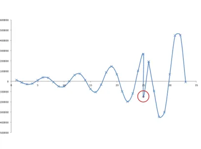
1. Point Anomaliesare single, outstanding data points that do not conform with the remain-der of the data. As an example, consiremain-der Figure 2.1. The green and purple dots are considered point anomalies, since they differ from the normal data points. Detecting point anomalies in a data set is rather simple, since it is sufficient to define some kind of metric or static measurement and apply it to the data. There is no need to set the data points in relation to each other or to know about the structure of the data set as a whole. 2. Contextual anomalieson the other hand, are single data points or groups of data, that are outstanding only when seen in context to other, surrounding data points or data structures. These anomalies are much harder to detect, because they are only considered anomalous in a specific situation, like, for example, they are appearing at a position in time or space where they are actually not supposed to be. If these data points were looked at individually, without any contextual relation, they would not be anomalous. To detect these points, it is therefore necessary to have extended knowledge about the structure and behavior of the system. Figure 2.2 provides an example data set with a data point that is anomalous when seen in context to the structure of the remaining data (data point marked red in the diagram).
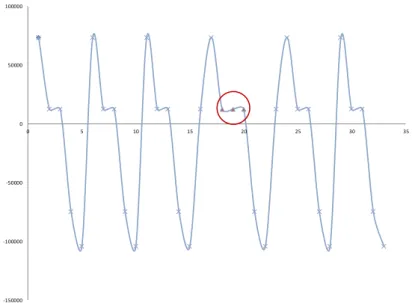
3. Collective anomaliesat last, are groups of data that are considered anomalous compared to the remaining data set. The data points in the collection itself do not necessary have
2. Foundations and Technologies 0 200 400 600 800 1000 1200 0 100 200 300 400 500 600
Figure 2.1.Example of anomalous single data points.
-500000 -400000 -300000 -200000 -100000 0 100000 200000 300000 400000 500000 600000 0 5 10 15 20 25 30 35
Figure 2.2.Contextual Anomaly - The red data point is anomalous in the context of the data structure.
2.1. Types of Anomalies -150000 -100000 -50000 0 50000 100000 0 5 10 15 20 25 30 35
Figure 2.3. Collective Anomalies - The red data points form a collection that is anomalous when compared to the rest of the data structure
to be anomalous, the occurrence as a group at a specific position however leads to an anomalous structure. Figure 2.3 provides an example for this type of anomaly. As can be seen, the collection of data points in the center of the diagram (marked red) form a group of anomalies.
Especially when it comes to analyzing log files, contextual and collective anomalies might be of strong interest for the user. Detecting these structures is related to the concept of
Event Correlation- according to [Sahoo et al., 2004], it is likely that periodically repeating events or long-term correlation effects (relation with events that happened a log time ago) are frequently occurring in log files. When applied to log files, events that occur within a similar time, close range or are occurring periodically might be related to each other. Especially when events do not contain important data individually but are important for the user because of the constellation they are in, these types of structures are hard to detect.
Example:Consider the following events: 1: INFO Reading file A (MsgId: 1) ...
2: ERROR Bad file descriptor (File A) ...
2. Foundations and Technologies
Each of the above events on their own do not contain enough information to let the user fully understand what is going on: The third event logs the occurrence of an error while processing file A. It is however unclear what error actually caused the system to fail - many other causes like an error in the processing routine could have been the reason for this event. The second event tells the user that a bad file descriptor caused an error regarding file A. Since there is however no ID coming with the error, it is not possible to relate the event to a location in the code. Lastly, the first event states, that the system is going to read file A. This message does whatsoever not contain any information about an error since it was generated before any error occurred. When all three events are related to each other, the source of the error (ID 1, file A), the cause (bad file descriptor) and the consequence (processing error in file A) can easily be found out. This information makes it easy to understand, locate and correct the error. The same applies for anomaly detection: Looking only on single events might not lead to the detection of these correlated events. Therefore, it is necessary to identify correlation structures in the file and group the anomalies according to these correlations.
2.2
Analysis Techniques
There are quite a lot analysis techniques for anomaly detection that have been developed in order to solve different problems in various fields of applications. The following presents two approaches that are related to this work.
Clustering-based techniques
Clustering based approaches perform a categorization of data points in a set in order to retrieve different partitions which can then be analyzed separately [Leung and Leckie, 2005; Chandola et al., 2009]. There are different approaches for clustering-based anomaly detection, basically, they can be split up into four groups.
1. Density-based techniquescluster the data into groups according to the density of a certain region. Therefore, each data point in a cluster has to be near a certain amount of other points within the cluster [Leung and Leckie, 2005].
2. Grid-based techniquesdefine several cells or hypercubes in the set of data, which then are used to cluster the space into groups of interest [Leung and Leckie, 2005]. 3. Centroid-based techniques assume that anomalous data points are not within close
range of cluster centroids [Chandola et al., 2009]. These techniques detect anomalies by evaluating how far away a single data point is from a cluster centroid. If the distance exceeds a certain threshold value, the data point is considered anomalous. 4. Nearest Neighbor-based techniques: Techniques that are based onnearest neighbor
ap-proaches assume that all normal data points are located close to each other while all
2.3. Principal Component Analysis (PCA)
other data points are considered anomalous [Chandola et al., 2009]. Therefore, simple nearest neighbor based approaches are not capable of detecting contextual or even collective anomalies in data sets. However, there are approaches that use complex metrics in order to enhance the process of finding contextual anomalies [Boriah et al., 2008]. There are also approaches that first cluster the data set with an appropriate clustering algorithm, for example the k-nearest neighbor algorithm and prune all clusters that cannot be anomalous. The anomalies are then calculated based on this condensed set [Ramaswamy et al., 2000].
Classification-based techniques
These techniques decide about anomalous data by evaluating whether or not the data instance belongs to a cluster [Chandola et al., 2009]. Therefore, only a special set of clustering algorithms that allow some data points not to be in any cluster can be used for this approach. Classification-based clustering techniques are commonly supervised, since the algorithm needs to learn how to differentiate between anomalous and normal data points.
2.3
Principal Component Analysis (PCA)
“In summary, PCA captures dominant patterns in data to construct a (low) k-dimensional normal subspace Sd in the original n-k-dimensional space. The remaining (nk)dimensions form the abnormal subspace Sa. By projecting the vector y on Sa (separating out its component on Sd), it is much easier to identify abnormal vectors. This forms the basis for anomaly detection.”Xu et al. [2009]
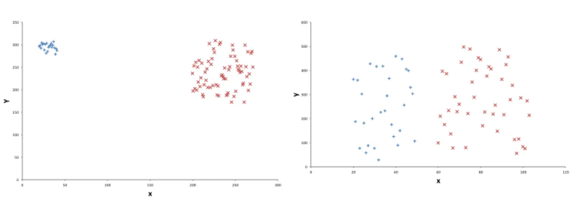
PCA can be used to structuralize and simplify large data sets with high dimensions. It is commonly used in image processing tasks but also in various other fields of application like information retrieval or text mining where it is important to reduce the raw amount of available data in order to come to a result in an acceptable time. In the context of detecting anomalies in log files, PCA can help to filter frequently repeating patterns in the data which makes it easier to detect anomalies. Basically, PCA finds dimensions that have the largest variances and sorts the dimensions in such a way that the first dimension contains the largest portion of the total variance and the last dimension the lowest portion [Ding and He, 2004]. In order to reduce the dimensionality, the last dimensions in the vector space can therefore be omitted after PCA has been applied, since those dimensions contain no valuable information. As a requirement for PCA, it is necessary, that all clusters have a lower variance within themselves compared to the variance between the clusters, since this would result in picking the wrong dimension (that contains little or no information at all) as illustrated in Figure 2.4
2. Foundations and Technologies 0 50 100 150 200 250 300 350 0 50 100 150 200 250 300 Y x
(a)Little variance within the cluster, high vari-ance between the clusters. The algorithm would order the x-dimension before the y-dimension (which contains no information about the clus-ters). 0 100 200 300 400 500 600 0 20 40 60 80 100 120 y x
(b)High variance within the cluster, little vari-ance between the clusters. The algorithm would order the y-dimension before the x-dimension (which contains more information about the clusters).
Figure 2.4.PCA example for two dimensions.
Therefore, when the principal components analysis is applied to a numeric data set, the first dimensions that will be removed are those that contain little to no varaiance. Therefore, the information loss when removing those dimensions is as little as possible. In fact, the removal of dimensions that have a small variance might even lead to better results since these dimensions consist mostly of noise and would therefore reduce the weight of dimenions that contain more information.
2.4
Clustering
This section will present different clustering techniques that can be applied to a data set in order to detect certain points of interest. The goal is to find a clustering algorithm that is able to reliably cluster the data set without the need of a labeled training set.
2.4.1
K-Means
The k-means clustering algorithm is commonly used for cluster analysis since it is fast and rather easy to implement. The algorithm tries to find groups of data instances with similar size and low variance [Kanungo et al., 2002]. Given a number k and an initial set of cluster centroids, standard k-means first assigns each data instance in the set to the nearest
2.4. Clustering
centroid using the euclidean metric. It then calculates a new centroid for each cluster by computing the means between all data points in the cluster. These two steps are repeated recursively until the centroid for all clusters does not change anymore. The K-Means algorithm is closely related to the k-Medoids algorithm that will be explained below and the k-center problem [Kanungo et al., 2002; Agarwal and Procopiuc, 2002] that tries to minimize the overall distance from the center to every other data point. According to [Mahajan et al., 2009], the K-Means problem is NP-hard and therefore no efficient solutions for solving this problem are known. The common procedure for the k-means problem is to iteratively execute the algorithm until a local minimum has been found [Kanungo et al., 2002]. This process is usually referred to as the k-means algorithm[Kanungo et al., 2002; MacQueen et al., 1967]. The algorithm is based on the assumption that the best center point for a cluster is the center of the cluster itself [Kanungo et al., 2002]. Of course, this assumption can lead to a high distortion of the center point when some data points in the cluster lie far away from the rest of the data points. Several approaches like the k-medoids try to reduce this effect. Because of the popularity of this algorithm, there are quite a few extensions to it that try to improve the precision and performance of the approach, like for example the k-means++ algorithm that tries to find better starting points or the k-medoids algorithm.
2.4.2
K-Medoids
The k-medoids algorithm [Arora et al., 1998] is a variation to the k-means algorithm mentioned above. The clustering algorithm chooses a set of k data points to represent the k clusters in the collection in such a way, that the data points that are not selected to be representative points can be clustered by evaluating the minimum distance between the data point and all the representative objects [Chu et al., 2002]. The data point then belongs to the cluster of the representative point with minimal distance. The general procedure of the algorithm is as follows (cf. [Chu et al., 2002]):
1. Arbitrarily choose an initial set Mof k-medoids
2. Create a new set Mnewby swapping one of the data points in the old set ofMwith a
data set in the collection for which the total distance from the points in the collection to
Mnewis the lowest possible. Then setM:=Mnew
3. Repeat step 2 until no point in M changes anymore. Then save the data points and terminate the program.
The algorithm is considered to be more robust compared to the standard k-means approach, mainly because a medoid is less influenced by noise and outstanding data points than the mean score. The disadvantage with this approach is, that the calculation is less time-efficient than the calculation of standard k-means.
2. Foundations and Technologies
2.4.3
X-Means
The X-Means approach extends the standard K-Means by computationally determining the numbers of clusters to be created and additionally by speeding up the whole algorithm itself [Pelleg et al., 2000]. The main problems with the standard K-Means implementation is, that it does not scale well for larger data sets and that the number of clusters have to be specified manually [Pelleg et al., 2000]. There are several other approaches that simply rerun the standard algorithm for different values of k to solve the second problem. This however still takes a lot of time to execute and might result in finding bad, local optima. According to Pelleg et al. [2000], the X-Means algorithm produces better results, since the algorithm is able to dynamically change the number of k in the process. Basically, the algorithm optimizes the Bayesian Information Criterion (BIC) by choosing the number of clusters and the position of the cluster centroids in the data set. The K-Means algorithm is used for selecting the best subset of data points that is then refined in a further step (for more details, see [Pelleg et al., 2000]).
2.5
Tools
Since anomaly detection is a well researched and often used technology, there are a lot of frameworks and tools that can be used for data clustering, data representation, etc. The goal of this work is to create and evaluate different number representations and anomaly detection algorithms. The framework used in this work was chosen to be the Kieker framework (see Section 2.5.3). Weka is used for data visualization and clustering whereas ELKI provides several anomaly detection algorithms that are used for evaluating the different data representations and algorithms.
2.5.1
Weka
Weka1is a well known tool for machine learning and statistical analysis that is written in Java and licensed under the GNU General Public License. Weka provides both a java library that can be used within the code itself as well as a graphical user interface to access its various functionalities. It is mostly used for machine learning tasks such as data classification or for educational purposes. Amongst others, its features include data visualization, cross-validation, data clustering and data classification [Holmes et al., 1994]. The Weka Library workbench is completely open source and since April 2000 entirely rewritten in Java, including the implementations of all algorithms [Hall et al., 2009]. In this work, Weka will be used for data clustering as well as for creating the principal components in some approaches and visualizing the result sets.
1http://www.cs.waikato.ac.nz/ml/weka/
2.5. Tools
2.5.2
ELKI
ELKI2(Environment for DeveLoping KDD-Applications Supported by Index-Structures) is a framework for knowledge discovery in databases that is mostly used in research areas [Achtert et al., 2008]. Many data mining algorithms are quickly forgotten again after being presented. According to Achtert et al. [2008], the reason for that is, that the implementations for the algorithms are not available and that they cannot be fairly compared with each other. ELKI provides therefore a standardized schema for implementing these data mining algorithms so that they can be better compared with each other [Achtert et al., 2008]. The ELKI framework is open source and written in Java. It consists of a graphical user interface and several data mining algorithms, as well as a Java Library. The algorithms provided are mostly algorithms for data clustering, classification, item-set mining and outlier detection [Achtert et al., 2008]. In this work, the outlier detection algorithms of the ELKI framework will be used for evaluating the constructed data sets and anomaly detection algorithms created.
2.5.3
Kieker Framework
The Kieker framework is a powerful framework that can be used to monitor software runtime behavior and the inner structure of software systems [van Hoorn et al., 2009, 2012]. It was built in order to be modular, extensible and flexible [van Hoorn et al., 2012]. The framework is open source and can be used for Java applications. Basically, Kieker consists of three different parts:
1. The Monitoring components gather the input data that will be observed. By default, Kieker already provides several monitoring probes, e.g. for collecting memory usage or CPU data [van Hoorn et al., 2012].
2. The collected data will then be written into a data storage by using the Monitoring Writer component [van Hoorn et al., 2012].
3. The last part of the framework will then analyze the data by reading the monitoring data collected in the previous step.
The main idea of the structure in Kieker is the concept of analysis chains which can be created by connecting different plugins with each other. This is especially useful for classification purposes or machine learning algorithms since these techniques process a data collection sequentially. The framework is designed so that it produces a low overhead for each processing step and therefore allows many iterations to be executed in the program.
2. Foundations and Technologies
2.6
Outlier Detection Algorithms
This section describes the anomaly detection algorithms that will be used for evaluation and comparison. The implementation of the following algorithms are taken from theELKI
Framework. The algorithms are applied to the three different number representations described in Section 3.3.
2.6.1
LOF
LOF (Local Outlier Factor) is an outlier detection algorithm that calculates the degree to which a data point is anomalous [Breunig et al., 2000]. The local outlier factor for a data point is calculated by analyzing the neighborhood around that data point which is done by measuring the density in this neighborhood. Basically, the algorithm consists of two steps: First, a local density measure for a data point is calculated to approximate the density of the neighborhood. This is done by computing the inverse average reachability distance between the current data point and all other data points in the neighborhood. Equation 2.1 shows the computation of the local reachability density for a specified parameter k.
lrd(a) = (∑bPNk(a)reachability_distk(a,b) |Nk(a)|
)(1) (2.1)
Thereachability distancebetween two data points is defined as the maximum of either the real distanced(a,b)between the two data points or thek-distanceof b. Nk(a)is a shortcut
for Nkdistance(a)(a). In principle, thek-distanceis the distance between a data point and another point, so that a certain amount of neighbor data points have an equal or less distance to the data point than that distance. A more detailed description of the formula can be found in the work by Breunig et al. [2000].
The second step of the algorithm is to create the LOF-value for all data points based on the approximated local density for each point.
LOFk(a) =
∑bPNk(a)lrd(b) |Nk(a)|
1
lrd(a) (2.2)
As can be seen in Equation 2.2, theLocal Outlier Factoris the average reachability distance of all neighbors of adivided by the actual reachability distance of the data point itself. Henceforth, if for a data point a LOF is computed that is approximately 1, it means, that the density in the region of that data point is comparable to the average density of the data points in the neighborhood. A value greater than 1 indicates on the contrary, that the density around the data point is lower compared to the average density in the neighborhood. The lower the density gets, the more outstanding the position of this data point will become. Therefore, a relatively high LOF indicates local anomalous data points in that region.
2.6. Outlier Detection Algorithms
The fact, that the LOF values are computed using only a local section of data points is very beneficial in data sets with varying density regions. Simple outlier detection algorithms would not be able to differentiate between these regions and would therefore misinterpret the regions with lower density as anomalous. Since there are no geometrical functions used in the algorithm, various different metrics that are not required to fulfill the triangle inequality can be applied to the approach easily.
The main problem of the LOF outlier detection algorithm is however the result interpreta-tion. The only output of the algorithm are LOF-values for each data point. A value that is greater than 1 does however not necessarily mean, that the data point is anomalous. In data sets with a high density deviation between the data points, a value greater than 2 might be related to a normal data point. On the other hand, for data sets with almost equally distributed data points, a value greater than 1.2 might already indicate a significant anomaly.
2.6.2
KNNOutlier
The KNNOutlier algorithm is agrid-basedanomaly detection approach for mining distance-based outliers [Ramaswamy et al., 2000]. The concept of the algorithm is to create partitions in the data sets which are then analyzed separately. As soon as the algorithm has deter-mined, that a partition cannot contain any outliers, the whole partition is pruned. Other partitions are analyzed for outliers which are classified based on the distance to their neighbors.
The main idea for the algorithms is the (slightly changed) definition from Knox and Ng [1998]: “A point in a data set is an outlier with respect to parameters k and d if no more than k points in the data set are at a distance of d or less from p.”(cf. [Ramaswamy et al., 2000]). An algorithm that is implemented to exactly match this definition would however face three problems that are difficult to solve:
1. The definition of the parameterd is hard to determine. An approximate good number may only be found by trial-and-error approaches like iteratively repeating the algorithm with different values ford.
2. The algorithm would only be able to classify the data points into two categories ( anoma-lousandnon-anomalous). Determining the degree of outlierness of a data point would be impossible.
3. cell-based approaches that have linear complexity do not scale with a high number of dimensions. Determining the data points by distancedwould therefore be complicated for high dimensional data.
To fix these problems, the KNNOutlier algorithm uses thek-nearest neighbor approach instead of the raw distances. The outlier ranking is done by sorting the data points based on the distance to itskth nearest neighbor. That way, the user can clearly see in the end
2. Foundations and Technologies
results to what degree a data point is anomalous compared to its neighborhood. As a solution to the expensiveness of algorithms with similar implementations, Ramaswamy et al. [2000] developed a partition-based approach in order to analyze the data set faster. The main idea is, that, in order to retrieve the topnoutliers, data points with a very small distance to their kth nearest neighbor do not have to be included in the analysis since there is no way that these points can be outliers. According to Ramaswamy et al. [2000], these distances can be approximated without actually computing the precise values by partitioning the data set which may result in a significant performance increase due to I/O as well as computation savings. The steps for partitioning are as follows (for a detailed explanation, see [Ramaswamy et al., 2000]):
1. Partition Computation: A clustering algorithm determines the partitions used in the following steps.
2. Approximation of the KNN bounds within each partition: The lower and upper bounds of the k-nearest neighbor distances in the partitions are calculated.
3. Relevant partition identification: All partitions that may contain outliers are selected in this step.
4. Outlier detection in candidate partitions: In every relevant partition, the outlier detec-tion algorithm is being executed.
By following these steps, a big portion of data points can be filtered out from the data set before running the actual outlier detection routine.
2.6.3
SOF
The spatial outlier factor (SOF) is a spatial outlier detection algorithm that is designed to be efficient and able to distinguish spatial (like locations, etc.) and non-spatial (text, statistical data, ...) dimensions [Huang and Qin, 2004]. Similar to LOF, this algorithm will also produce afactor, i.e. a degree to which a data point is anomalous.
The computation of SOF consists of two steps: The first step is to calculate the local density
ldfor a data point. This is computed through Equation 2.3.
ld(a) = |impact_neighborhood(a)|
∑bPimpact_neighborhood(a)attrdist(a,b)
(2.3) whereimpact_neighborhood(a)is a list of neighbors foradetermined by a reflexive and sym-metric spatial relation and attr_dist(a,b)the distance betweenaandbin an n-dimensional euclidean space (for more information, see [Huang and Qin, 2004]). The local density of a data point atherefore is the inverse average distance of the neighbor data points toa. The next step is to calculate the spacial outlier factor for the data point. Equation 2.4 shows
2.6. Outlier Detection Algorithms
the computation of the SOF value.
SOF(a) =
∑
bPimpact_neighborhood(a) ld(b) ld(a) 1 |impact_neighborhood(a)| (2.4) If the SOF value for a data point is high, it means, that the local density around that point is low compared to the density of the neighbors of that data point. Therefore, the higher the SOF for a data point, the more likely it is, that this data point is an outlier.2.6.4
ODIN
TheOutlier Detection using Indegree Number (ODIN)algorithm uses the k-nearest neighbor graph in order to determine outlier data points [Hautamäki et al., 2004]. The main idea is to calculate a kNN graph withunidirectionaledges and determine theindegreefor all odes in the graph. If the indegree is lower than the threshold parameterT, the data point will be marked as an outlier. The kNN graph hereby is a weighted, directed graph that represents all data points as vertexes. Every vertex has exactlykedges to itsk-nearest neighbors. The weight of an edgeei,jis the distance between the vertexvi andvj, which is provided by the
distance function. the ODIN algorithm uses an extended version of this kNN graph where the graph has an edge betweenviandvj if the original kNN graph has both an edge from vi tovj and en edge fromvjtovi.
Chapter 3
General Approach
This chapter will give detailed insight in the solution finding process as well as the developed techniques used in this approach. The chapter is structured into four parts that explain each step of the general approach individually, starting with the description of the developed number representations, followed by the data filtering, data clustering and anomaly detection part.
3.1
Overview
The general idea of the algorithm is to group different data points into one single instance in order to find anomalous structures in the data set. Common approaches for anomaly detection mostly focus on the analysis of contextual relationships between single data points or, in the case of cluster-based approaches, between data points and clusters. The algorithm developed in this work especially focuses on the relation between different groups of data points and is therefore an approach that tries to detect outstandingareas
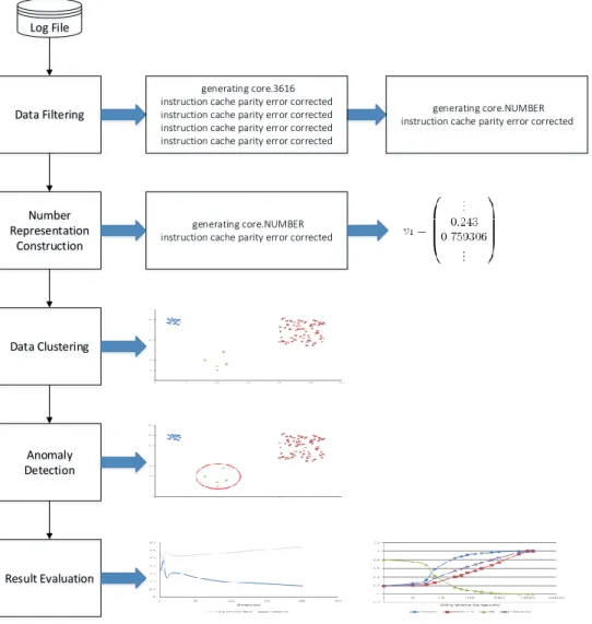
in the data set. The general approach of this work consists of five different steps (see Figure 3.1):
1. Thefilteringstep (Section 3.2) reduces the amount of events that are considered in the next steps. This step is crucial for the further analysis because it reduces the amount of redundant messages in the collection. This way, every message in the filtered data set gains more weight and importance and the created blocks of events become more significant.
2. The next step is to create thenumber representation(Section 3.3) of the events in the filtered collection. This is another crucial step in order to get decent results when detecting the anomalous data points. In this step, every event, respective every block of events, is assigned a vector that represents the content of the events. This work will evaluate three different number representation approaches in order to determine which of them is the most applicable for this type of data.
3. Based on the number representations created in the previous step, the data can then be processed by adata clusteringalgorithm (Section 3.4). This step may be skipped by the
3. General Approach
external algorithms that will also be used for anomaly detection. The anomaly detection approaches developed in this work will however be executed on the clustered collection. The main reason to cluster the data set is to detect the different types of events.
4. Theanomaly detectionstep (Section 3.5) then analyzes the preprocessed data set and detects potential outliers in the collection. For this purpose, several external outlier detection algorithms and one outlier algorithm developed in this work will be used together with the three developed number representations.
5. The final step is theresult evaluation(Chapter 5), where the different number represen-tation approaches and anomaly detection algorithms will be compared.
3.2
Data Filtering
Finding and removing duplicate or unrelated events that contain no information in a log file as a preprocessing step can be beneficial for further steps like the number representation generation. Merging or removing these events from the log file significantly reduces the number of event messages that need to be analyzed. When filtering a data set, it is very important to recognize possible correlation structures that might occur within the set. If certain events are in relation with each other, it might be crucial to analyze them as a whole. Therefore, deleting these events should be avoided when filtering the data set.
There are several approaches for filtering textual data like log files - the used techniques can basically be categorized into two groups, “Temporal Reduction” and “Spatial Reduc-tion”.
3.2.1
Temporal Reduction
The temporal reduction of events is based on the assumption, that events which were produced within a short time period, are likely to be coming from the same error [Tang et al., 1990]. Events of the same type, coming from the same source are merged into a single event within a short time span. Depending on the particular algorithm, different types of events within close range produce several different merged events. Choosing the time span in which these events are merged needs to be analyzed for each data set individual. Choosing a very long time span might result in merged events that have nothing particular in common while choosing the time span to short, duplicate messages will not be filtered out.
3.2. Data Filtering Log File Number Representation Construction Data Clustering Anomaly Detection Result Evaluation Data Filtering generating core.3616
instruction cache parity error corrected
instruction cache parity error corrected
instruction cache parity error corrected instruction cache parity error corrected
generating core.NUMBER
instruction cache parity error corrected
generating core.NUMBER
instruction cache parity error corrected
3. General Approach
3.2.2
Spatial Reduction
Distributed systems pose another challenge for filtering event logs. Logs may be gathered across a large number of different machines and centralized for a better analysis of the whole system [Liang et al., 2005]. The log events from these machines can be spatially correlated with each other in order to filter or merge messages that were caused by the same error but were distributed by several nodes in the system. If a failure is occurring on different machines in a distributed system, the error produced by these nodes can lead to multiple other errors in other nodes that were not the source of the error. With temporal filtering alone, these errors cannot be detected since they might be emitted from different nodes.
Spatial filtering can be done for example by defining a causal order of events and creating a graph that represents the event transmissions within the system nodes [Zheng et al., 2009]. By analyzing the relations between the vertexes in the graph, a spacial filtering algorithm might be able to associate the different events with each other and remove spacial duplicates.
3.2.3
Adaptive Semantic Filter
The filtering technique used in this work in order to preprocess the BlueGene/L log file is called theAdaptive Semantic Filter (ASF), which was developed by Liang [2007]. The implementation that is used in this thesis was developed by Pitakrat et al. [2014]. The disadvantage of most of the temporal and spacial filtering techniques is, that they require a deep understanding of the domain they are used in and that they often need a human operator in order to deal with new types of events [Liang, 2007]. Furthermore, simple techniques that use thresholds for identifying temporal or spatial relations are often not suitable to handle more complex situations and can produce wrong results [Liang, 2007]. The procedure of the ASF-filtering method basically consists of three steps: The first step is to create a keyword dictionary that contains all keywords contained in the input file. The keywords can be iteratively appended to the dictionary while filtering the data set. All encountered event descriptions will be normalized using several transformation rules like replacing hexadecimal numbers by a keyword or removing punctuations, prepositions or articles.
The second step is to create a number representation for every event, which is a binary vector that contains one dimension for each keyword. Every dimension is related to a particular keyword and the value of a vector at the respective position represents whether or not that keyword is contained in the event description.
The third and last step is to apply the ASF-filter by computing a correlation value that determines the relationship of an event to another event, known as theφ-correlation [Liang,
2007; Reynolds and Reynolds, 1977]. Based on this correlation coefficient, the adaptive
3.3. Data Representation
semantic filtering is applied. The main idea behind this filtering is, that events that are close to each other but differ more in their descriptions might still be related to each other, whereas events that have the same description but are temporarily far away might already be unrelated since they are likely to come from two different sources.
3.3
Data Representation
A very important element in finding outstanding structures in the data set is to compute a representation for the points within the collection. When gathering information out of textual data like the description of a particular log entry, there are many steps necessary in order to achieve a result that is able to represent the extracted information in an acceptable way. Numerical representations of a text should be able to determine which data points are similar to each other. Good representations therefore maximize the distance between dissimilar data points and minimize the distance for similar or equal text values. That way, classification algorithms are able to distinguish between the different kinds of data structures within a collection.
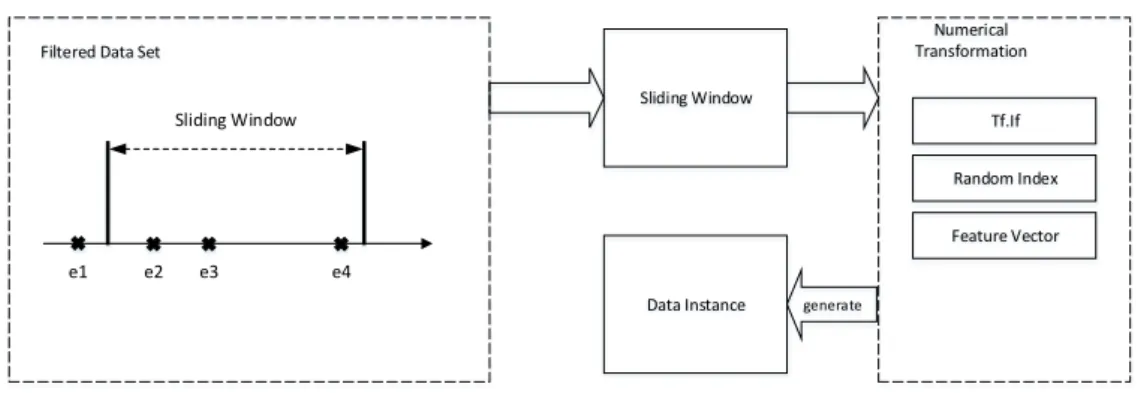
In this work, three different number representation algorithms are developed (described in the following). The main idea behind each of them is to group multiple events from the log file together and represent them as a single data point. This is done by sequentially reading the log file and storing a certain number of events into a collection (called the
sliding window) while reading through the data set. When a new eventenewis read from
the log file, the sliding window contains the new event and all previously read events that are “near” enew. Both the Tf.Idf number representation (Section 3.3.1) as well as the Feature Vector number representation(Section 3.3.3) allow the sliding window size to vary. Therefore, for these two approaches, the sliding window contains all previously read events that are within a certain time span, thesliding window size. If the sliding window size is for example 300 seconds, the sliding window contains all previously read events where|time_stamp(enew)time_stamp(e)| ¤300 holds. For theRandom Index representation
(Section 3.3.2), the sliding window size cannot be varied since the number of events grouped together represents the number of dimensions for this data point. Therefore, the sliding window for this approach contains always the same number of events.
Figure 3.2 shows the general process for creating numerical data points (data instances). Based on the filtered data set, the program is sequentially reading the data points. For every new event read, the sliding window is updated so that is always contains related events. Next, the data representation algorithms are executed which transform all the data points in the sliding window into one numerical data instance. These data instances are stored and used in the next steps.
3. General Approach
Sliding Window Filtered Data Set
Numerical Transformation
Tf.If Random Index Feature Vector
Data Instance generate
Sliding Window
e1 e2 e3 e4
Figure 3.2.General process for creating data instances.
3.3.1
Tf.Idf Representation
A common approach for the numerical transformation of textual data is to represent the textual information as multidimensional Tf.Idf (term frequency, inverse document frequency) vectors. These values are relatively easy to extract, since it is only necessary to create a mapping from the term itself to the overall occurrence of the term in the data set. In a second preprocessing step, the Tf.Idf values can then be computed for each event. The extracted feature vector, which has one dimension for each relevant term, can then be used as a comparator to decide which events are similar and which are not. This is usually achieved by some kind of distance measure, like for example the euclidean distance. The approach of using Tf.Idf vectors for the retrieval of textual information is very common in information retrieval when it is necessary to retrieve textual information that is structured as chunks of data like documents in a large collection [Aizawa, 2003]. The idea of Tf.Idf is to determine the frequency (relative to the collection) of a word in a certain document while words that do not occur in very many documents have a higher Tf.Idf value than words that occur very frequently [Ramos, 2003]. The Tf.Idf value consists of two components: the first component, called term frequency, measures the number of occurrences within the document. The second component, called inverse document frequency, represents the rareness of a term relative to the collection. When multiplying these two values, the intuitive result is a measure of the relevance of a term in a specific document.
The mathematical definition of the Tf.Idf value varies from application to application, but a common definition would be like the following (c.f. [Ramos, 2003]). Given a collection of documentsD, an arbitrary word w, and a particular documentdPD, the term frequency of a document is calculated as shown in Equation 3.1
d fd(term) =
∑
tPTerms(d)equals(term,t) (3.1)
3.3. Data Representation
where Terms(d P D) consists of all terms that are contained in the document and
equals(term,t)is defined as in Equation 3.2.
equals(a,b) =
0 ,i f a ¡b
1 ,i f a=b (3.2)
The document frequency computes how many documents contain a specific word. It is therefore defined as the folowing.
d fd(term) =|{d:dPDXtermPTerm(d)}| (3.3)
Finally, the Tf.Idf value is computed as shown in Equation 3.4
t f.id f(term,d) =t fd(term) | D| d fd(term)
(3.4) It is simple to apply the Tf.Idf values to log files by splitting up the file into blocks of events which are then considered documents. An enhanced approach would be to overlap the groups by a certain rate in order to better detect structural anomalies that are located between two blocks. This can be achieved by implementing a sliding window that, beginning with the first event in the log file, groups events that are temporally close to each other. By advancing the sliding window with the next event that has to be processed, it ensures, that all events in the current event collection of the window that have a timestamp difference of more than the threshold value are removed again from the collection. For every event in the log file, this changing collection can then be directly used as a document and the Tf.Idf values can be computed out of that group. Figure 3.3 visualizes the idea of the Tf.Idf computation.
Steps of the algorithm
Step 1: Calculate the term frequency for each term.
Step 2: The sliding window returns a group of temporally close events.
Step 3: The Tf.Idf values are computed for each event in this group
Step 4: The values are added component-wise. This is equivalent to calculating the Tf.Idf values from the group as a whole, but the advantage in adding the values component-wise and calculating them for each term separately is that the values can be computed in a separate preprocessing step.
Step 5: In a post-processing step, the generated numerical data set will be compressed by using the principal components algorithm described in Section 2.3.
3. General Approach generating .36 core .28 data .23 ... ... ... ... Term Value Term-Tf-Idf Mapping Add Componentwise
INFO RAS generating core.2800 INFO RAS generating core.10 INFO RAS generating core.33 INFO RAS generating core.45 FATAL RAS data TLB error interrupt FATAL RAS data TLB error interrupt FATAL RAS data TLB error interrupt FATAL RAS data TLB error interrupt INFO RAS generating core.62 INFO RAS generating core.3626
(.36 .28 0 0 0) INFO RAS generating core.2800 (.36 .28 0 0 0) INFO RAS generating core.10 (.36 .28 0 0 0) INFO RAS generating core.33 (.36 .28 0 0 0) INFO RAS generating core.45 (0 0 .54 .23 .76 .20) FATAL RAS data TLB error interrupt (0 0 .54 .23 .76 .20) FATAL RAS data TLB error interrupt (0 0 .54 .23 .76 .20) FATAL RAS data TLB error interrupt (0 0 .54 .23 .76 .20) FATAL RAS data TLB error interrupt (.36 .28 0 0 0) INFO RAS generating core.62 (.36 .28 0 0 0) INFO RAS generating core.3626
Figure 3.3.Basic idea of the Tf.Idf approach.
Advantages and Disadvantages of Tf.Idf Advantages:
events with high Tf.Idf scores impact the values the most.
The more infrequent, rare terms in a group, the higher the value will get.
The groups can vary in size - temporal correlations can be considered.
Disadvantages:
Use for online analysis might be difficult since all vectors and clusters have to be updated when a new word appears.
Dimensionality of the vector space depends on the number of terms in the data set. The dimensionality might have to be compressed by using techniques like principal component analysis.
Inverted Index Construction
An inverted index is a data structure that is used to map a term to a collection of doc-uments that contain the term (so calledpostings list) [Cutting and Pedersen, 1989]. This data structure is used in the tf.idf approach to efficiently compute the inverse document frequency values. In the context of application in this work, a single event in a log file is here considered a document. Therefore, in the tf.idf algorithm, every event or block of event (depending on the number representation settings) in the log file is seen as a individual document and the values are computed individually for each event(-block).
3.3. Data Representation
3.3.2
Random Indexing Representation
The Tf.Idf representation above can only be used for larger data sets, if the number of dimensions is significantly reduced, for example by using the principal component analysis or by using special processing algorithms for sparse data. Reducing the dimension of the data can be very slow, especially when the data set does not fit into the memory anymore while sparse data always comes with the problem of processing high dimensional data (curse of dimensionality).
The random index representation solves the problem of high-dimensional vectors. The random indexing creates only one single value to represent an event in the log file (in contrast to the Tf.Idf approach that creates|Terms|dimensions for one event). Therefore, for analyzing contextual anomalies, several events in the log can simply be combined by creating a vector where each dimension represents one event. The number of dimensions is then related to the block size for which the events are grouped into one instance. Given a set of eventsE, the algorithm first creates a random numberRtfor all terms in the
collection. After removing irrelevant terms (e.g. frequent terms or stop words) from this mapping, the algorithm then computes for each event a representative number by adding all the random numbers in the event into one value.
R(ePE) =
∑
tPTermse
Rt (3.5)
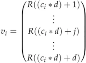
After computing these values for all events in the collection, the next step is to group every block of events created by the sliding window into a vector of the sizedto enable contextual analysis of the data. The resulting vectorvi can then be used for further steps
(clustering, anomaly detection). Equation 3.6 shows the computation of the vectorviPNd
for the blockci PNin the collection.
vi= R((cid) +1) .. . R((cid) +j) .. . R((cid) +d) (3.6)
Figure 3.4 illustrates the process of creating the random index representation.
Advantages and Disadvantages of Random Indexing Advantages:
The algorithm produces only one dimension for one event. The dimensionality is therefore independent of the grammar in the data set.
3. General Approach generating 100 core 8934 data 503 ... ... ... ... + Term Value Term-Value mapping +
INFO RAS generating core.2800 INFO RAS generating core.10 INFO RAS generating core.33 INFO RAS generating core.45 FATAL RAS data TLB error interrupt FATAL RAS data TLB error interrupt FATAL RAS data TLB error interrupt FATAL RAS data TLB error interrupt INFO RAS generating core.62 INFO RAS generating core.3626
9034 INFO RAS generating core.2800 9034 INFO RAS generating core.10 9034 INFO RAS generating core.33 9034 INFO RAS generating core.45 2533 RAS data TLB error interrupt 2533 RAS data TLB error interrupt 2533 RAS data TLB error interrupt 2533 RAS data TLB error interrupt 9034 INFO RAS generating core.62 9034 INFO RAS generating core.3626
Figure 3.4.Basic idea of random indexing.
The dimension of a data point in the resulting collection can be adjusted by the user. A higher dimension correlates to the detection radius for contextual anomalies.
The temporal ordering of events can be considered - it is possible to detect chronologi-cally outstanding anomalies.
New words do not lead to new dimensions. An online approach can be realized with little effort.
Equally rare terms are differentiated - Tf.Idf representations thread equally frequent words as the exact same word.
No sparse data, no need for dimensionality reduction algorithms.
Other dimensions that are added to the data set have greater impact (e.g. a separate dimension for the severity of an event, or even user-defined new dimensions for any kind of data)
Disadvantages:
Rare terms have no effect on the score. All terms are equally rare.
Frequent terms therefore have to be filtered out in a preprocessing step.
The number of events in one representation has to be static. This is an important disadvantage because events in a filtered log file may vary much in their temporal distance to their neighbors.
3.3. Data Representation
3.3.3
Feature Vector Representation
Another approach for representing the events in the log files as numerical values is to choose the dimensionality of the vector space so that it matches the number of event types in the log file. A number in a particular dimension then represents the occurrence of that type of event in the current block. Figure 3.5 visualizes this approach. The red box represents the current position of the sliding window in the log file. The figure demonstrates how the dimensions are retrieved in the log file and how the resulting vectors are generated. In the example, the log file consists of 4 different event types. Therefore, generated vectors for each event has four dimensions. The sliding window contains five events of the third event type and two events of the fourth event type. The resulting numerical representation is therefore the vectorv = (0, 0, 5, 2)T. By filtering out event
4 Dim e n sio n s Log File
INFO RAS CE sym 10, at 0x1b9d4000, mask 0x04
INFO RAS total of 1 ddr error(s) detected and corrected INFO RAS generating core .2800
INFO RAS generating core .10 INFO RAS generating core .33 INFO RAS generating core .45 FATAL RAS data TLB error interrupt FATAL RAS data TLB error interrupt FATAL RAS data TLB error interrupt FATAL RAS data TLB error interrupt INFO RAS generating core .62 INFO RAS generating core .3626 INFO RAS generating core .219 INFO RAS generating core .456 INFO RAS generating core .2795 INFO RAS generating core .2682 FATAL RAS data TLB error interrupt FATAL RAS data TLB error interrupt
Figure 3.5. General idea of the feature vector representaation. The log file consists of 4 different event types, therefore 4 dimensions are generated. The vector representation is computed for each block of events (sliding window).
types that do not occur a certain number of times in the log file, the number of dimensions can be reduced. The Evaluation in Chapter 5 will filter out event types for which there are less than five occurrences in the log file. However, with only this possibility of dimension reduction, the approach still needs to be post-processed by using the principal components to reduce the dimensions even more.
3. General Approach
Advantages and Disadvantages of the Feature Vector Representation Advantages:
The groups can vary in size - temporal correlations can be considered.
The number of dimensions can be reduced by filtering out event types with low occur-rence.
New dimensions can simply be appended to the vector - if a new type of event occurs in the data set, the representation does not have to be rebuilt again.
Disadvantages:
Dimensionality of the vector space depends on the number of event types in the data set. The dimensionality might have to be compressed by using techniques like principal component analysis.
The rareness of events cannot be represented with this approach.
3.4
Data Clustering
Data clustering will be used in some of the algorithms analyzed in this work. There are many clustering algorithms available that can be used for the approach in this work, how-ever, not all are equally suited for the task. The following criteria should be fulfilled: 1. The number of clusters are unknown. The clustering algorithm should therefore be able
to automatically determine the number of clusters on its own.
2. There are many data points in the data set. Therefore the clustering algorithm has to be fast and scalable. The overhead produced should be as low as possible.
3. The clustering must be able to create a decent categorization of the items contained in the data set.
As already explained in Section 2.4, the X-Means algorithm is able to determine the number of clusters and quickly cluster the data set and will therefore be used for the clustering task.
3.4.1
Advantages of data clustering
The main reason to cluster the data set is to split the events into groups of different event types. A log file usually contains many different kinds of messages that might occur at different frequencies in the collection. This however does not necessarily mean that those
3.5. Anomaly Detection
data points are more anomalous than the more frequent occurring ones. By clustering the data points, the goal is to split these messages up so that they can be analyzed individually. This procedure might force the anomaly detection algorithm to value the constellation of the events more than the different types of messages and therefore could consider contextual relationships better.
Example:Consider a system that is iteratively executing three steps: 1. Read input
2. Compute data 3. Generate result
In either of these steps, there are most likely different event messages that are occurring only in this step. If however the computation of the data is the most complex step, there will presumably be much more events that are related to the data computation part in the log. Since the anomaly detection algorithm will especially mark rare events or event constellations as anomalies, it is possible that the events that are emitted in the other two steps will be considered anomalous. By clustering the data points, these three steps can be separated from each other under the right conditions. The clustered data can then be analyzed separately for the three different steps and errors within them can be detected better.
Another reason for data clustering is, that the amount of data that will be compared with each other gets reduced. This could be especially important for log files with a very large amount of events.
3.5
Anomaly Detection
This section describes the approach for the developed position-based anomaly detection algorithm. The algorithm presented in the following is developed in order to determine how important the clusters in log file-like data sets are. The idea behind the concept is, that each cluster defines an area of similar data relations. As explained in Section 3.3, the numerical representations group temporal related events into one data instance. These data instances are meant to represent the contextual difference between every instance, i.e., they represent thecontextof a group of events at a given position in the log file. The contextcn of a data instancedinis defined by the types of events that are contained in the
instance as well as by the temporal relations between these events. Therefore, a cluster contains data instances with similar event type constellations (i.e. instances with similar events), that is, with similar contexts. If a data instance is far away from the cluster center, the hypothesized reason is, that the context of the area defined by the data instance is in some way outstanding. This might be due to rare events, but can also be caused by an outstanding constellation of events within this area. The more unusual the constellation
3. General Approach
or the events within the data instance, the farther away it gets from the majority of events with similar contexts. Equally, clusters that consist of only a few data points define areas of outstanding context. Even if the distances to the center is very small, data instances within a tiny cluster have to be considered anomalous too.
Most of the existing outlier detection algorithms analyzed in this work use k-nearest neighbor distances in order to evaluate how outstanding a data instance is. This approach however utilizes the cluster centers as “idealized” area contexts that represent the ap-proximated standard-context for the data instances contained in the cluster. The distance
d(din):=diidealdinrepresents how ordinary the data instancedinin contrast to the “ideal”
data instance is. Using the k-nearest neighbors, the calculated distance between a data instancedinand its neighbors would only represent the density arounddin. If the same
context occurs more than once, the local density will get higher in the respective position ofdin. This however does not necessarily mean, thatdin is not anomalous, since reports of
faulty processes are usually not reported just once in the whole log file but are reported multiple times. The kNN distance would therefore not represent the outlierness of the data instance but only determine, whether similar context structures have ever happened in the log file. As mentioned before, determining the “ideal” data point will be done by running a data clustering algorithm. Since the K-Means algorithm clusters the data by approximating the center point as an average of all data points in the cluster, this approach might be the best choice for determining those data points.
The proposed algorithm in this section determines the distances to the cluster center for each data instance as described above. Similar to the LOF outlier detection, the algorithm outputs a degree to which a data instance is anomalous. The following presents two approaches for an anomaly detection algorithm that uses the cluster center to determine the outlierness of data points.
3.5.1
A Position-Based Anomaly Detection Algorithm
The first approach is to order the data instances in each cluster based on their distance to the cluster center. This order is then used to determine the level to which the data instance is anomalous. The farther away the data point is from the center, the higher the position in the order gets. In order to identify data points in a tiny cluster, the algorithm first computes theglobal outlier level (gol)that indicates how large the cluster is in which the current data point is contained in.
The global outlier level for a clusterCin a data setDis defined as
gol(C) =P(xRC) =1P(xPC) =1|C|
|D| (3.7)
3.5. Anomaly Detection
The outlier level of a data point d in its clusterCdis then computed as outlierLevel(d) = position(d)
|Cd|
gol(Cd) (3.8)
The global outlier level returns a higher value when the current clusterC contains few data points and a lower value if the cluster contains many points. It therefore can be seen as a global weight factor for all clusters in the collection. The term position|C (d)
d| computes
the local outlierness of a data point within clusterCd. The farther away the data point is
from the center of the cluster, the higher theoutlierLevelbecomes. Therefore, the closer the outlierLevel is to 1, the more anomalous the data point is. Similar to LOF, there is however no constant threshold foroutlierLevelthat determines between anomalous and non-anomalous data points. It is therefore required to specify the threshold or the number of anomalies manually.
3.5.2
Extension: Including the Rareness of Events using Tf.Idf
In extension to the algorithm above, the following approach describes another way of detecting outliers in log files. Since the random index approach as well as the feature vector approach do not consider the rareness of the events, it might be a good idea to include the term rareness in the process of detecting anomalies.
LetS be the set of data points andAbe the set of anomalous data points withAS. In order to determine the degree to which a data point is anomalous, two factors have to be considered:
1. The level of outlierness of a specific data point (see Equation 3.8) 2. The textual rareness of an event in the context of all other events
Therefore, the level to which a data instance v P S is anomalous could be defined as follows: anomalyLevel(v) =rareness(v)outlierLevel(v) (3.9) whererareness(v)determines the rareness of all terms contained invandoutlierLevel(v) represents a measure of how much the data instance is outstanding compared to the rest of the data.
The rareness of a data pointvPSis defined as
rareness= ∑ |v| i=0∑| Terms(v)| j=0 t f.id f(vi,j) maxxPS ∑|iv=|0∑| Terms(v)| j=0 t f.id f(vi,j) (3.10)
whereTerms(x)represents all relevant terms of a single event andt f.id f(x)represents the term/document frequency as shown in Equation 3.11.
3. General Approach
t f.id f(term,v) = (
∑
tPTerms(v)
equals(term,t))(log| |S|
{x:xPS^termPTerm(x)}|+1) (3.11) equals= 0 ,i f a ¡b 1 ,i f a=b (3.12)
Since the rareness of events is already included in the Tf.Idf data representation, the extension might be viable only for the two other number representations. The rareness extension adds a third weight to theoutlierLevelfactor and is computed by considering the global outlierness of a cluster, the local position of a data point within that cluster and the rareness of the events contained in the data point.