Essays in Asset Pricing
!
!
Keywan Rasekhschaffe!
University of Lugano!
!
!
A dissertation submitted for the degree of!
Ph.D. in Economics!
!
!
!
!
!
!
!
!
Thesis Committee:!
Prof. Stephen H. Penman, Columbia University!
Prof. Giovanni Barone Adesi, University of Lugano!
Prof. Francesco Franzoni, University of Lugano!
Prof. Eric Nowak, University of Lugano!
This dissertation examines a series of asset pricing “anomalies” and investigates links to
fundamentals. In the first chapter I investigate the gross yield effect. Gross yield, defined as gross
interest expense divided by liabilities, has power comparable to book- to-market and firm size in
predicting the cross-section of returns. Firms with low gross yield are found to earn higher
returns than firms with high gross yield. This effect is significantly more pronounced when
controlling for book-to-market since gross yield and book-to-market are positively correlated but
predict returns with the opposite sign. The gross yield effect is difficult to reconcile with
explanations of the value premium because high gross yield firms are more prone to distress and
also tend to have high book-to-market ratios. This effect is robust to various factors related to
distress and other characteristics known to have power in the cross-section. Gross yield survives
controls for book-to-market, size, momentum, profitability, and a host of proxies for distress.
Investors can significantly reduce the risk of value strategies by taking on exposure to gross
yield. !
In the second chapter we examine the link between average returns and cash-flow risk. This
paper investigates cashflow risk and its relationship to average returns. We find that stocks with
earnings that co-vary strongly with market-wide earnings also earn a high return. The cashflow
beta (or earnings beta) of value stocks is found to be much higher than that of growth stocks, and
small stocks have higher cashflow betas than large stocks. Thus, cashflow betas can explain a
significant part of the Fama and French factors. This provides evidence for a risk-based
explanation of anomaly returns because stocks earning a higher return also tend to have riskier
cashflows.!
In the third and final chapter I analyze an anomaly in the cross-section of FX volatility. This
paper studies the cross-section of foreign exchange volatility returns. Statistically and
economically significant returns are produced by a zero-cost trading strategy that is long (short)
volatility swaps on currencies with high (low) historical volatility relative to implied volatility.
The spread portfolio has a Sharpe ratio in excess of 1.7, results are robust to different market
conditions and time periods, and it remains highly profitable after transaction costs. Standard risk
adjustments do not significantly diminish profitability because the strategy is only weakly
correlated with the equity market, the carry trade, and the Fama-French risk factors. Moreover,
the historical-minus- implied volatility (HMI) factor also predicts excess-returns of the
underlying currencies. Currencies that have high historical volatility relative to their implied
volatility have much higher returns.!
The Gross Yield E↵ect
Keywan Christian Rasekhscha↵e⇤June 5, 2014
ABSTRACT
Gross yield, defined as gross interest expense divided by liabilities, has power comparable to book-to-market and firm size in predicting the cross-section of returns. Firms with low gross yield are found to earn higher returns than firms with high gross yield. This e↵ect is significantly more pronounced when controlling for book-to-market since gross yield and book-to-market are positively correlated but predict returns with the opposite sign. The gross yield e↵ect is difficult to reconcile with explanations of the value premium because high gross yield firms are more prone to distress and also tend to have high book-to-market ratios. This e↵ect is robust to various factors related to distress and other characteristics known to have power in the cross-section. Gross yield survives controls for book-to-market, size, momentum, profitability, and a host of proxies for distress. Investors can significantly reduce the risk of value strategies by taking on exposure to gross yield.
JEL classification: F31; F37;G10;G11.
⇤. I thank Giovanni Barone-Adesi, Francesco Franzoni, Eric Nowak and Stephen H. Penman. I am also grateful
I.
Introduction
Gross yield, defined as gross interest expense divided by liabilities, has power comparable to book-to-market in predicting the cross-section of returns. Previous research extensively documents a positive relationship between many proxies for value and expected equity returns. In stark contrast, gross yield is negatively correlated with future equity returns. To my knowledge this is the first study to document a negative relationship between gross yield on firm liabilities and expected equity returns.
A positive relationship between several proxies for value and returns has been widely docu-mented. It is well known that the earnings-to-price ratio is positively related to returns. More recently Novy-Marx (2013) documents that gross profits-to-assets predicts returns, and the book-to-market e↵ect is widely documented both when considering the equity portion alone as well as when considering enterprise-wide book-to-market (Nissim and Penman (2003)). What I find is in stark contrast to earlier research: a negative relationship between yield and subsequent returns. Empirically, returns to my gross yield strategy are strongly correlated with the Fama and French (1992) factors HML and SMB as well as an earnings-to-price factor. Thus, these returns are puz-zling when examined through the lens of the Fama and French (1992) three factor model. Also, gross yield correlates strongly with measures of distress and negatively forecasts earnings growth.
The empirical association between measures of yield and expected returns on the same asset has been extensively documented. Hansen and Hodrick (2007); Fama (1984) show that currencies with higher interest rates have higher returns than currencies with low yield interest rates. Gorton, Hayashi, and Rouwenhorst (2013) document a forward discount bias for commodity futures, and Campbell and Shiller (1988) show that dividend price ratios forecast equity index returns.
Gross yield focuses solely on accounting liabilities in the denominator and thus di↵ers from traditional proxies for value which typically involve scaling by price. Gross yield is strongly related to the yield on long-term debt: high correlation of gross yield with earnings-to-price, and theoretical models based on the intuition that debt and equity are merely di↵erently structured claims on the same underlying asset suggest that the required return on debt and equity be positively correlated. Empirical studies on the relationship between equity and debt returns have found that they are positively correlated (Kwan (1996); Blume, Keim, and Patel (1991)). It is necessary to test if
returns of my gross yield strategy are due to indirectly sorting on characteristics which could drive yield spreads. Indeed, the gross yield e↵ect persists when controlling for the characteristics that determine the relationship between equity and debt returns of the same firm. While these factors do not explain the e↵ect, the negative association of gross yield with future returns is more pronounced among both low volatility and low leverage firms. Collin-Dufresne, Goldstein, and Martin (2001) find that equity returns and yield spread changes are less correlated in practice than might be expected. They find that only a small portion of credit spreads can be explained by firm-level variables, which suggests a disconnect between debt and equity markets. In any case, a contingent claim analysis might only be partially relevant to the gross yield anomaly because not all liabilities are traded and the denominator of gross yield includes operating liabilities as well as financial liabilities.
Previous research argues that the profitability of value strategies is mechanical, since firms that require a higher rate of return have lower prices. For example Berk (1998) and Ball (1978) argue that accounting ratios involving price pick up on higher expected returns because they identify firms with depressed prices. Berk (1998) argues that the low price is justified because of risk. Behavioral explanations also suggest that accounting variables scaled by price identify low priced stocks (Lakonishok, Shleifer, and Vishny (1994)). However, they argue that high expected returns of these stocks are due to mispricing due to behavioral biases of investors. When either argument is applied to the gross yield e↵ect, a positive relationship between gross yield and average returns would be expected: high gross yield indicates high expected returns. Contrary to this intuition, firms with higher gross yield produce markedly lower returns than firms with lower gross yield. They do so despite having higher book-to-market ratios and smaller size. Double sorts on gross yield and book-to-market suggest that gross yield e↵ectively helps identify “bad” value: high book-to-market stocks that also have high gross yield have much less impressive returns than high book-to-market stocks with low gross yield.
Double sorts on size and gross yield suggest that the gross yield e↵ect is present in all size quintiles. This suggests that the gross yield e↵ect is also economically relevant and not only present amongst small or micro capitalization stocks. Moreover, the anomaly is unlikely to be explained by transaction costs, since gross yield is a highly persistent metric, with results being only slightly weaker if gross yield is lagged an additional year.
II.
Yield and the cross-section of expected returns
Gross yield is distinct form the yield on debt claims since it scales interest by total liabilities. However, yield on debt and gross yield are strongly correlated. Structural models like Merton (1974) and related models such as Longsta↵ and Schwartz (1995); Black and Cox (1976); Leland (1994) and Collin-Dufresne et al. (2001) suggest that debt and equity returns on the same firm should be positively correlated under most circumstances. In Merton’s model the debt claim is essentially a combination of a risk-free debt claim and a short position in a put option on the firm at the value of the risk-free claim. The model specifies a firm value process and assumes that default is triggered at the maturity date if the face value of debt is larger than firm value. In the case of default, debt holders receive the residual firm value instead of face value. If the probability of default is zero, the put option is worthless and the debt claim issued by the firm behaves like a risk-free bond. As the probability of default increases the debt claim is largely composed of the short put option. If a default event is very likely, and the expected residual firm value is low, then debt should be more equity-like. If the probability of default is low and residual firm value high, debt should behave more like a risk-free bond.
Chen, Collin-Dufresne, and Goldstein (2009) suggest that credit spreads are defined by firm value, the risk-free rate, and several “other state variables” related to expected default. To the present analysis firm-level state variables are the most relevant since they might explain cross-sectional di↵erences in gross yield. Macro-variables like the level of interest rates are less important to this analysis since they a↵ect all securities. The most important firm-level variables from the literature that determine the probability of default are:
1. Leverage: higher leverage increases the probability of default. Therefore it should be expected that debt of high-leverage firms is more equity-like. In order to control for leverage I control for of debt/(debt + market value of equity).
2. Profitability: higher profitability decreases the probability of default. Firms earning higher returns on their assets can a↵ord to pay higher interest rates on their debt. Therefore it should be expected that debt of high-profitability firms is less equity-like. In order to control for profitability I control for the ratio of gross profits to gross assets.
increases the value of the put option and therefore the debt of highly volatile firms should behave more like equity. In order to control for volatility I use the 250-day standard deviation of equity returns.
4. Probability of downward jumps: the higher the probability of a downward jump, the less residual value bond holders are expected to recover in the event of default. Unfortunately the probability of downward jumps is not easily observable without a cross-section of option prices for each firm. Only a small number of firms have reliable data on implied volatility smirks. Therefore, I rely on skewness of returns measured over the past 250 trading days. 5. Past returns: firms facing default typically experienced poor past returns. I aim to control
for this by controlling for past 12 month returns. I would expect gross yield to be more informative about expected stock returns for firms with poor recent returns.
A. Fama-MacBeth regressions
Table I presents time-series averages of Spearman rank correlations and shows that gross yield is positively correlated with book-to-market. Table II shows results of Fama and MacBeth regressions of firm gross yield controlling for book-to-market, size and past performance over twelve months. I use Compustat data from the inclusion of the American Stock Exchange (Amex) in 1962 and assume all accounting data is available in June of the following calendar year. Thus, tests cover the sample period from 1962 to 2010. Table III also presents results for gross yield when the variable is demeaned by median industry values. For industry definitions I use the Fama and French (1997) 49 industry portfolios.
The first specification in Table II shows that gross yield has power comparable to the Fama and French factors book-to-market and size in predicting the cross-section of returns. The second specification replaces gross yield with yield on long-term debt. Yield on long-term debt has vir-tually no power in predicting returns. In the third specification, I include earnings-to-price which can be interpreted as the equity counterpart to gross yield. The slope on gross yield remains vir-tually una↵ected while earnings-to-price has the expected positive sign. The fourth specifications adds 12-month momentum, which also does not diminish the significance of gross yield. The fifth specification includes leverage, to ensure the power of gross yield is not due to implicitly sorting on this variable. Finally, the sixth specification includes all controls and gross yield maintains a
highly significant T-statistic of -4.27 in this case.
Even though leverage is closely related to gross yield, specifications 5 and 6 show that controlling for this characteristic does not eliminate the performance of gross yield. Also, volatility and jump risk do not appear to be responsible for predictive power of gross yield. In the context of the Merton (1974) model, 12-month momentum is also expected to be related to gross yield as distressed firms with high gross yield can be expected to have much poorer returns than firms with low gross yield. Since momentum predicts returns, it is reassuring that the inclusion of the momentum variable does not eliminate the power of gross yield.
It is known that industry-adjusted characteristics often perform better (see e.g.: Asness, Porter, and Stevens (2000)). Table III repeats the previous analysis with industry-adjusted analysis. As expected, the T-statistic for book-to-market increases. Gross yield, however, does not perform better: for all specifications the raw yield metric is a more successful predictor. For completeness Table IV repeats the analysis with industry-wide metrics. While book-to-market becomes almost insignificant, gross yield has power comparable to the industry-adjusted metric, suggesting that both industry-wide and industry-adjusted variation in gross yield are valuable for predicting returns.
B. Sorts on gross yield
The Fama and MacBeth regressions of Table II allow a glimpse at the predictive power of gross yield. However, they weight small caps and micro caps very heavily. Also, they are very sensitive to outliers and rely on a parametric model that might well be misspecified, which makes the results difficult to judge. In this section I examine equal-weighted and value-weighted portfolios sorted on gross yield providing a non-parametric test of the pricing power of gross yield in the cross-section. Table V shows results for univariate sorts on gross yield. Gross yield and book-to-market are highly correlated and therefore high gross yield firms should outperform low yield firms since they are value stocks. Portfolios are formed using a quintile sort based on New York Stock Exchange (NYSE) breakpoints. The table reports average excess returns, as well as alphas and factor loadings obtained from regressing portfolio returns on the Fama and French factors. Moreover, time-series averages of gross yield (GY), book-to-market (BM), and market capitalization (ME) are reported. The sample includes financial firms and I verify, in unreported results, that results change little if
the highest yield portfolio earning 0.08 percent per month lower average returns than the portfolio with the lowest gross yield firms. The high-low spread portfolio has a monthly Fama and French alpha of -0.36 percent and a highly significant T-statistic of -4.12. The Fama and French alpha has a higher T-statistic than the slope for gross yield in cross-sectional regressions. It appears that returns of the gross yield strategy are more correlated with HML and SMB factor returns, than the gross yield characteristic is correlated with book-to-market and firm size. However, this di↵erence partially arises because cross-sectional regressions do not control for the market factor. High gross yield firms are value stocks, meaning that they have high book-to-market ratios, while low gross yield firms are growth stocks in the sense that they have low book-to-market ratios. Despite high gross yield firms returns behaving like value stocks as well as having similar characteristics, they have lower expected returns. This leads to the Fama and French alphas of the spread portfolio being much higher than the raw returns.
C. Yield and size
Value-weighted returns presented in Table V already suggest that the strategy is economically significant and not exclusive to small caps and micro caps. In this section I further show that results are robust to firm size by performing double portfolio sorts on gross yield and market capitalization. Portfolios are formed by independently sorting on size and gross yield, using NYSE breakpoints. The sample covers from 1963 to 2010.
Table VI also reports the characteristics of size portfolios which show modest variation in gross yield with larger stocks having slightly less gross yield. Table VI also reports characteristics of gross yield portfolios.
Table VI reports returns for double-sorted portfolios on size and gross yield. The gross yield e↵ect is present across all size quintiles and is almost as strong amongst the largest stocks as it is for the smallest stocks. Table VI also reports intercepts and their T-statistics from regressions of these returns on the Fama and French factors. The di↵erence in returns and Fama and French alphas is present amongst all size quintiles. This shows that the gross yield e↵ect is economically relevant even amongst the largest firms.
III.
Yield and value
Table I shows that the correlation coefficient between gross yield and book-to-market is positive. Since gross yield predicts returns in the opposite direction, the two characteristics should comple-ment each other. Table VII presents results which suggest that traditional value strategies can be improved by controlling for gross yield. Value strategies are far more profitable if they exclude stocks that have very high gross yields and instead focus on firms that have low-to-moderate gross yield. Similarly, a univariate gross yield strategy can be improved by incorporating book-to-market: firms with low gross yield are much more profitable if they also have high book-to-market ratios.
A. Double sorts on gross yield and book-to-market
This section examines these conjectures by analyzing the performance of portfolios double-sorted on book-to-market and gross yield. Portfolios are formed by independently sorting on these two variables, again using NYSE break points. The sample ranges from 1963 to 2010. Table VII presents average returns as well as Fama and French alphas and factor loadings for high-minus-low portfolios. Moreover, the table shows the average number of stocks in each portfolio as well as average firm size.
Low gross yield firms outperform high gross yield firms across all book-to-market quintiles. As expected, book-to-market does not explain gross yield returns, and each book-to-market and yield strategies are stronger when controlling for the other. The results confirm the hypothesis that controlling for gross yield significantly improves the performance of the book-to-market strategy. The average value spread across gross yield quintiles is much larger than the univariate spread portfolio for book-to-market.
B. Large cap gross yield and value
Results from Table VI indicate that gross yield has power even amongst the largest stocks. In this section I restrict the sample to the 500 largest stocks as measured by market capitalization at the end of December each year. Table XII shows results from cross-sectional Fama and MacBeth regressions on this sample. The predictive power of all variables is greatly diminished albeit gross yield, book-to-market and size still predict returns with the same sign.
Table XIII shows results for univariate sorts on gross yield. Gross yield and book-to-market are highly correlated and therefore high gross yield firms should outperform low gross yield firms since they are value stocks. Portfolios are formed using a quintile sort. This table reports average excess returns, as well as alphas and factor loadings obtained from regressing portfolio returns on the Fama and French factors. Moreover, time-series averages of gross yield (GY), book-to-market (BM), and market capitalization (ME) are reported. The sample includes financial firms. I verify in unreported results that results change little if financial firms are excluded.
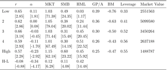
The spread portfolio still has negative average returns and the Fama and French alpha is -0.34 percent per month and highly significant with a T-statistic of -4.17. Increases in gross yield are associated with higher loadings in particular on HML, but also SMB, again suggesting that high gross yield firms behave like value stocks in covariances. Also characteristics support this, with high gross yield firms being significantly less profitable and having much higher book-to-market ratios than low gross yield firms.
Table XIV presents double sorts for book-to-market and gross yield focusing exclusively on the 500 largest stocks. Value and gross yield strategies amongst the largest stocks are highly negatively correlated. Therefore, it is not surprising that Fama and French alphas are negative across all book-to-market quintiles.
C. Large cap yield and value strategy
The high negative Fama and French alphas already suggest the complementary relationship between gross yield and book-to-market. Firms with high book-to-market and low gross yield tend to be “good” value stocks, with much higher performance than high book-to-market and high gross yield. Table XIV presents a gross yield strategy that is long in low gross yield stocks and short in high yield stocks. An investor combining the value and gross yield strategies can significantly reduce the risk of a pure book-to-market strategy because returns of the gross yield strategy are negatively correlated with a book-to-market strategy. As a result the combined strategy has a T-statistic of 5 and a Sharpe ratio of 0.72 which is well above the Sharpe ratio for the market portfolio over the sample period despite only trading the largest stocks.
Figure 1 shows the performance of the combined yield and book-to-market strategy. The figure presents the three year rolling Sharpe ratio over the preceding three years at the end of each month
from 1963 to 2010 (represented by the dashed line). The figure also shows the trailing Sharpe ratio for a book-to-market strategy and a 50/50 mixed strategy. The mixed strategy has a much higher T-statistic (x)and Sharpe ratio than the value and gross yield strategy each have individually.
While both the value and gross yield strategies did have solid performance over the sample period, both su↵ered significantly for long periods of time. The mixed strategy has much more consistent performance and did not have a losing year.
IV.
Portfolio sorts
In this section I control for several other characteristics that have power in the cross-section. Also, I examine robustness to characteristics that determine relative expected returns of debt and equity. The Merton (1974) model suggests that several factors related to the probability of default, and expected recovery rates in the event of default, should determine the extent to which debt and equity are correlated. Moreover, these factors also are expected to determine the magnitude of yield spreads: we would expect gross yield to be more correlated with equity returns for firms that have riskier debt. Analyzing gross yield and factors related to firm risk jointly provides a way to test if this can be observed. Moreover, I need to ensure that the returns on gross yield portfolios are not achieved by implicitly ranking on these theoretical drivers of yield spreads.
A. Double sorts on gross yield and leverage
Table V shows that high gross yield portfolios also have higher leverage. This is not surprising since other things equal, increasing leverage makes debt more risky and thus increases gross yield. In Table VIII, I examine how controlling for leverage a↵ects the pricing power of gross yield. With the exception of the highest leverage quintile, high-minus-low portfolios formed on gross yield have negative alphas. While a closer relationship between required returns for debt and equity are expected for risky stocks, it remains unclear why gross yield and expected equity might be negatively related in the lower four leverage quintiles.
Interestingly returns increase in leverage when controlling for gross yield. However, since the leverage metric includes price, this is perhaps not too surprising. Results from Table II suggest that once we control for book-to-market, leverage provides no further valuable information in
predicting returns. Since Fama and French alphas of the high-minus-low portfolios are negative and significant for four leverage quintiles and insignificant for the highest leverage quintile, the results appear robust.
B. Double sorts on gross yield and idiosyncratic volatility
For firms at risk of default, expected returns on debt could be closely related to expected equity returns. Hence I would expect gross yield to be more highly correlated with equity returns amongst high volatility firms. Table IX reports returns for double-sorted portfolios on gross yield and volatility. Indeed the Fama and French alpha for the spread portfolio formed on gross yield is insignificant for the most volatile quintile. However, alphas are negative within all volatility quintiles and are significant within the other four. Similarly, returns are also negative for all quintiles except the most volatile. These results suggest that expected returns on debt and equity might be more closely related amongst firms with high volatility, however, the gross yield e↵ect is robust to controls for idiosyncratic volatility.
C. Double sorts on gross yield and skewness
Similarly, firms with lower skewness might have a closer relationship between debt and equity returns because, historically, they were at risk for large downward jumps. However, historical skewness has not always been a good predictor of future skewness. Table X reports results from double sorts on skewness and gross yield. The gross yield-based spread portfolios are negative for all five skew quintiles and returns for double-sorted portfolios on skewness and gross yield. Skewness is defined as the 250-day rolling skewness of returns updated each month. The gross yield e↵ect is present across all skewness quintiles. Fama and French alphas are negative and mostly significant with no discernible systematic variation based on skew. The gross yield e↵ect does appear robust to controls for historical skewness.
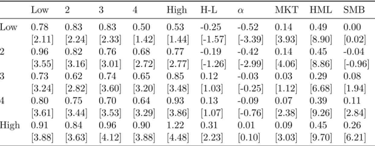
D. Double sorts on gross yield and profitability
Finally, I examine interaction of profitability and gross yield. Profitability is defined as gross profit (Compustat REVT-COGS) divided by total assets (Compustat item AT). Since more itable firms can a↵ord higher interest payments, their debt should be less risky. Moreover,
prof-itability is a powerful predictor in the cross-section. Table XI reports results from double sorts on profitability and gross yield. Fama and French alphas are negative for all but the most profitable stocks. Surprisingly, the gross yield e↵ect is strongest among the least profitable firms.
The gross yield e↵ect remains a puzzle and does not appear to be explained by factors related to distress. Even though Fama and French alphas are less significant among high volatility and leverage stocks, they are more significantly negative for low-profitability firms and unrelated to historical skewness even though these stocks might very well be at higher risk of default.
V.
Conclusion
The negative association between gross yield and returns is puzzling considering the empirically established notion that measures of value are positively associated with expected returns. Firms with high gross yield have lower returns despite having much higher book-to-market ratios and smaller size than low gross yield firms. Therefore, the results cannot be explained by the Fama and French three factor model and are difficult to explain with the Berk (1998) critique since gross yield can reasonably be expected to signal higher required return. Also, behavioral explanations relating anomalies to over-reaction do not explain the returns, since high gross yield firms exhibit continuation of low returns rather than mean-reverting. Importantly, the gross yield e↵ect is almost as pronounced among the very largest stocks. The fact that results are almost as strong when restricting the universe to the largest 500 equities by market capitalization suggests the anomaly has economic implications rather than being merely an interesting statistical pattern confined to small and hard-to-trade stocks. Empirically, gross yield adds significant information to traditional value. A strategy that is long low gross yield firms and short high gross yield firms is a growth strategy both in characteristics and covariances. Since the gross yield and value strategies are negatively correlated, they complement each other very well. Investors can significantly reduce the risk of value strategies by taking on exposure to the gross yield strategy. Value investors should therefore incorporate information about gross yield since this can dramatically decrease their risk. Moreover, the gross yield e↵ect is robust to various factors related to distress and other characteristics known to have power in the cross-section. Gross yield survives controls for book-to-market, size, momentum, profitability, and a host of proxies for distress.
REFERENCES
Asness, Cli↵, R Porter, and Ross Stevens, 2000, Predicting stock returns using industry-relative firm characteristics, Available at SSRN 213872 .
Ball, Ray, 1978, Anomalies in relationships between securities’ yields and yield-surrogates,Journal of Financial Economics 6, 103–126.
Berk, Jonathan, 1998, A critique of size related anomalies, Review of Financial Studies .
Black, Fischer, and John C Cox, 1976, Valuing corporate securities: Some e↵ects of bond indenture provisions, The Journal of Finance 31, 351–367.
Blume, Marshall E, Donald B Keim, and Sandeep A Patel, 1991, Returns and volatility of low-grade bonds 1977–1989, The Journal of Finance 46, 49–74.
Campbell, John Y, and Robert J Shiller, 1988, The dividend-price ratio and expectations of future dividends and discount factors,Review of financial studies 1, 195–228.
Chen, L, P Collin-Dufresne, and R S Goldstein, 2009, On the relation between the credit spread puzzle and the equity premium puzzle, Review of Financial Studies 22, 3367.
Collin-Dufresne, Pierre, Robert S Goldstein, and J Spencer Martin, 2001, The determinants of credit spread changes, The Journal of Finance 56, 2177–2207.
Fama, Eugene, 1984, Forward and spot exchange rates* 1, Journal of Monetary Economics 14, 319–338.
Fama, Eugene, and Kenneth French, 1992, The cross-section of expected stock returns,Journal of Finance 47, 427–465.
Fama, Eugene F, and Kenneth R French, 1993, Common risk factors in the returns on stocks and bonds, Journal of financial economics 33, 3–56.
Fama, Eugene F, and Kenneth R French, 1997, Industry costs of equity, Journal of financial economics 43, 153–193.
Gorton, Gary B, Fumio Hayashi, and K Geert Rouwenhorst, 2013, The fundamentals of commodity futures returns, Review of Finance 17, 35–105.
Hansen, Lars Peter, and Robert J Hodrick, 2007, Forward Exchange Rates as Optimal Predictors of Future Spot Rates: An Econometric Analysis,The Journal of Political Economy 88, 829–853.
Kwan, Simon H, 1996, Firm-specific information and the correlation between individual stocks and bonds, Journal of Financial Economics 40, 63–80.
Lakonishok, Josef, Andrei Shleifer, and Robert W Vishny, 1994, Contrarian investment, extrapo-lation, and risk, Journal of Finance 49, 1541–1578.
Leland, Hayne E, 1994, Corporate debt value, bond covenants, and optimal capital structure,The journal of finance 49, 1213–1252.
Longsta↵, Francis A, and Eduardo S Schwartz, 1995, A simple approach to valuing risky fixed and floating rate debt, The Journal of Finance 50, 789–819.
Merton, Robert C, 1974, On the pricing of corporate debt: The risk structure of interest rates*, The Journal of Finance 29, 449–470.
Nissim, Doron, and Stephen H Penman, 2003, Financial statement analysis of leverage and how it informs about profitability and price-to-book ratios,Review of Accounting Studies 8, 531–560.
Novy-Marx, Robert, 2013, The other side of value: The gross profitability premium, Journal of Financial Economics .
Figure 1. Rolling Sharpe RatiosPerformance over time of gross yield and value strategies. The figure shows the trailing five-year Sharpe ratios of gross yield and value strategies (blue and green lines, respectively) and a 50/50 mix of the two (red dashed line). The strategies are long/short extreme value-weighted quintiles from sorts on gross profits-to-assets and book-to-market, respec-tively, and correspond to the strategies considered in Table VII. The sample covers June 1963 to December 2010. Shaded areas are NBER recessions.
Figure 2. Cumulative Alpha per month after portfolio formation Persistence of yield strategy performance. This figure shows the average cumulative returns to the gross yield strategy considered in Table A6 from one to 25 months after portfolio formation. The sample covers January 1972 to December 2010
ab le I p ear m an ran k cor re lat ion s b et w ee n in d ep en d en t var iab le s. T h is tab le re p or ts th e ti m e-se ri es av er age s of th e cr os s se ct ion S p ear m an k cor re lat ion s b et w ee n th e in d ep en d en t var iab le s em p lo ye d in th e F am a an d M ac B et h re gr es si on s of T ab le 1: p rofi tab il it y [( R E VT -O G S )/A] , b o ok -t o-m ar ke t, m ar k et eq u it y, an d p as t p er for m an ce m eas u re d ov er 12 m on th s. T h e sam p le co ve rs fr om 1963 to 2010. YI E LD B M M V E P LE VE R M O M 12 S K E W 250 V O L250 YI E LD 1. 00 0. 12 -0. 07 0. 01 0. 31 -0. 05 0. 02 0. 05 B M 0. 12 1. 00 -0. 24 0. 14 0. 42 -0. 13 0. 03 0. 01 M V -0. 07 -0. 24 1. 00 0. 17 -0. 06 0. 07 -0. 25 -0. 47 E P 0. 01 0. 14 0. 17 1. 00 0. 15 0. 05 -0. 12 -0. 27 LE VE R 0. 31 0. 42 -0. 06 0. 15 1. 00 -0. 09 -0. 02 -0. 06 M O M 12 -0. 05 -0. 13 0. 07 0. 05 -0. 09 1. 00 0. 15 -0. 03 S K E W 250 0. 02 0. 03 -0. 25 -0. 12 -0. 02 0. 15 1. 00 0. 23 V O L250 0. 05 0. 01 -0. 47 -0. 27 -0. 06 -0. 03 0. 23 1. 00
Table II
Fama and MacBeth regressions of returns on measures of gross yield. This table reports results from Fama and MacBeth regressions of returns on gross yield (gross interest expense XINT scaled by liabilities LT). Regressions include controls for book-to-market [BM], size [MV], yield on long-term debt [YIELDLT], leverage [LEVER], earnings-to-price [EP] and past performance measured over 12 months [MOM12] and covers July 1963 to December 2010.
(1) (2) (3) (4) (5) (6) BM 0.28 0.18 0.23 0.23 0.34 0.23 [5.68] [2.96] [5.39] [5.55] [7.37] [6.61] EP 0.16 0.15 0.16 [3.01] [3.07] [3.31] MOM12 0.10 0.10 [2.22] [2.25] MV -0.17 -0.09 -0.19 -0.19 -0.19 [-2.20] [-1.07] [-2.70] [-2.80] [-2.82] YIELDLT 0.04 [0.74] YIELD -0.09 -0.09 -0.09 -0.09 -0.09 [-3.49] [-3.51] [-3.92] [-3.77] [-4.27] LEVER 0.03 -0.01 [0.68] [-0.37] INTERCEPT 0.79 0.63 0.80 0.81 0.80 0.81 [3.30] [3.25] [3.35] [3.39] [3.34] [3.40]
Table III
Fama and MacBeth regressions of returns on measures of gross yield demeaned by industry. This table reports results from Fama and MacBeth regressions of returns on gross yield (gross interest expense XINT scaled by liabilities LT). Regressions include controls for book-to-market [BM], size [MV], yield on long-term debt [YIELDLT], leverage [LEVER], earnings-to-price [EP] and past performance measured over 12 months [MOM12] and covers July 1963 to December 2010.
(1) (2) (3) (4) (5) (6) BM 0.27 0.22 0.24 0.24 0.28 0.21 [7.79] [4.35] [7.13] [7.43] [7.70] [7.43] EP 0.16 0.16 0.16 [4.37] [4.56] [4.66] MOM12 0.08 0.08 [2.36] [2.58] MV -0.16 -0.06 -0.18 -0.18 -0.18 [-2.59] [-1.03] [-3.15] [-3.23] [-3.22] YIELDLT -0.01 [-0.17] YIELD -0.05 -0.04 -0.04 -0.06 -0.07 [-2.25] [-2.04] [-2.33] [-3.07] [-3.86] LEVER 0.12 0.08 [3.78] [2.92] INTERCEPT 0.78 0.62 0.78 0.79 0.78 0.79 [3.26] [3.31] [3.24] [3.30] [3.27] [3.31]
Table IV
Fama and MacBeth regressions of returns on industry-level measures of gross yield. This table reports results from Fama and MacBeth regressions of returns on gross yield (gross interest expense XINT scaled by liabilities LT). Regressions include controls for book-to-market [BM], size [MV], yield on long-term debt [YIELDLT], leverage [LEVER], earnings-to-price [EP] and past performance measured over 12 months [MOM12] and covers July 1963 to December 2010.
(1) (2) (3) (4) (5) (6) BM 0.06 -0.02 0.07 0.09 0.08 0.06 [1.32] [-0.26] [1.66] [2.15] [1.65] [1.35] EP -0.05 -0.05 -0.05 [-1.11] [-0.99] [-1.03] MOM12 0.06 0.06 [1.49] [1.44] MV -0.09 -0.04 -0.08 -0.09 -0.10 [-1.95] [-0.63] [-1.78] [-2.14] [-2.46] YIELDLT -0.01 [-0.14] YIELD -0.08 -0.08 -0.08 -0.06 -0.07 [-2.05] [-2.18] [-2.26] [-1.45] [-2.02] LEVER -0.05 0.01 [-1.36] [0.16] INTERCEPT 0.75 0.69 0.75 0.76 0.74 0.75 [3.12] [3.33] [3.15] [3.21] [3.11] [3.21]
Table V
Excess returns to portfolios sorted on gross yield. This table shows monthly value-weighted average excess returns to portfolios sorted on gross yield [gross interest expense (XINT) scaled by liabilities (LT)] employing NYSE breakpoints, and results of time-series regressions of these portfolio returns on the Fama and French factors [the market factor (MKT), the size factor small-minus-large (SMB), and the value factor high-minus-low (HML)], with T-statistics (in square brackets). It also shows time-series average portfolio characteristics [portfolio gross profits-to-assets (GP/A), leverage, av-erage firm size (ME, in millions of dollars), and number of firms (n)]. The sample covers July 1963 to December 2010.
r ↵ MKT SMB HML GP/A BM Leverage Market Value
Low 0.83 0.27 0.95 0.82 -0.04 0.35 -0.67 0.28 1040029 [3.29] [3.08] [45.71] [28.31] [-1.24] 2 0.76 0.09 1.02 0.70 0.23 0.36 -0.55 0.38 3036227 [3.22] [1.34] [67.12] [32.98] [10.04] 3 0.77 0.08 0.99 0.59 0.36 0.31 -0.42 0.47 2098331 [3.52] [1.21] [66.83] [28.43] [16.16] 4 0.64 -0.07 0.99 0.62 0.38 0.28 -0.37 0.51 1375298 [2.86] [-1.02] [59.78] [26.95] [15.18] High 0.75 -0.09 1.04 1.01 0.41 0.27 -0.37 0.54 406517 [2.68] [-0.74] [37.59] [26.10] [9.77] H-L -0.08 -0.36 0.09 0.19 0.45 [-0.81] [-4.13] [4.52] [6.63] [14.50] Table VI
Double sorts on gross yield and market equity. This table shows the value-weighted average excess returns to portfolios double-sorted, using NYSE breakpoints, on gross yield and market equity, and results of time-series regressions of high-minus-low portfolio returns on the Fama and French factors [the market, size and value factors MKT, SMB (small-minus-large), and HML (high-minus-low)]. T-statistics are given in square brackets. The sample covers July 1963 to December 2010.
Low 2 3 4 High H-L ↵ MKT HML SMB Low 1.65 1.46 1.37 1.11 1.30 -0.36 -0.50 0.09 0.25 -0.00 [4.80] [4.36] [4.25] [3.55] [3.81] [-2.37] [-3.30] [2.44] [4.60] [-0.01] 2 0.64 0.84 0.97 0.62 0.55 -0.10 -0.41 0.17 0.47 0.17 [2.36] [2.86] [3.43] [2.32] [1.78] [-0.68] [-3.05] [5.36] [9.73] [3.96] 3 0.76 0.59 0.69 0.69 0.44 -0.32 -0.57 0.14 0.45 -0.03 [2.80] [2.20] [2.73] [2.60] [1.55] [-2.29] [-4.25] [4.49] [9.38] [-0.66] 4 0.69 0.69 0.58 0.46 0.40 -0.29 -0.51 0.12 0.44 -0.07 [2.72] [2.84] [2.59] [2.14] [1.52] [-2.23] [-4.17] [4.03] [9.94] [-1.77] High 0.50 0.49 0.50 0.48 0.30 -0.19 -0.40 0.05 0.36 0.11 [2.20] [2.42] [2.58] [2.53] [1.26] [-1.57] [-3.31] [1.87] [8.35] [2.72]
Table VII
Double sorts on gross yield and book-to-market. This table shows the value-weighted average excess returns to portfolios double-sorted, using NYSE breakpoints, on gross yield and book-to-market, and results of time-series regressions of high-minus-low portfolios returns on the Fama and French factors [the market, size and value factors MKT, SMB (small-minus-large), and HML (high-minus-low)]. T-statistics are given in square brackets. The sample covers July 1963 to December 2010. Low 2 3 4 High H-L ↵ MKT HML SMB Low 0.36 0.24 0.20 0.07 0.32 -0.05 -0.36 0.09 0.44 0.36 [1.28] [0.91] [0.75] [0.26] [0.96] [-0.29] [-2.27] [2.37] [7.81] [6.91] 2 0.74 0.61 0.50 0.43 0.43 -0.31 -0.44 0.03 0.20 0.13 [2.85] [2.58] [2.21] [1.93] [1.55] [-2.25] [-3.18] [0.97] [4.14] [2.84] 3 1.02 0.82 0.71 0.55 0.46 -0.56 -0.75 0.10 0.35 -0.01 [3.99] [3.45] [3.34] [2.56] [1.72] [-4.17] [-5.70] [3.33] [7.37] [-0.12] 4 1.06 1.05 1.13 0.89 0.88 -0.17 -0.35 0.13 0.26 0.03 [4.12] [4.08] [4.78] [3.78] [3.14] [-1.22] [-2.45] [3.92] [5.13] [0.60] High 1.56 1.39 1.45 1.21 1.39 -0.17 -0.41 0.15 0.30 0.22 [5.43] [4.86] [5.16] [4.31] [4.37] [-1.13] [-2.78] [4.32] [5.69] [4.59] Table VIII
Double sorts on gross yield and leverage. This table shows the value-weighted average excess returns to portfolios double-sorted, using NYSE breakpoints, on gross yield and leverage [book value of debt/(market value of equity+book value of debt)], and results of time-series regressions of high-minus-low portfolios returns on the Fama and French factors [the market, size and value factors MKT, SMB (small-minus-large), and HML (high-minus-low)]. T-statistics are given in square brackets. The sample covers July 1963 to December 2010.
Low 2 3 4 High H-L ↵ MKT HML SMB Low 0.62 0.34 0.27 0.16 0.21 -0.41 -0.40 -0.04 -0.11 0.28 [2.26] [1.28] [0.89] [0.48] [0.61] [-2.28] [-2.26] [-0.87] [-1.66] [4.72] 2 1.13 0.79 0.74 0.59 0.73 -0.40 -0.48 0.04 0.05 0.18 [4.24] [3.35] [3.17] [2.40] [2.46] [-2.59] [-3.08] [1.02] [0.83] [3.59] 3 1.17 0.91 0.72 0.68 0.65 -0.52 -0.65 0.14 0.17 -0.00 [4.31] [3.84] [3.41] [3.00] [2.42] [-3.26] [-4.03] [3.74] [2.90] [-0.06] 4 1.01 0.97 0.92 0.65 0.79 -0.22 -0.36 0.07 0.11 0.26 [3.72] [3.68] [4.10] [2.99] [2.89] [-1.21] [-1.94] [1.68] [1.70] [4.24] High 0.98 0.98 1.33 0.87 1.13 0.14 0.02 0.02 0.08 0.37 [3.21] [2.71] [3.79] [2.71] [3.21] [0.60] [0.06] [0.41] [0.88] [4.69]
Table IX
Double sorts on gross yield and return volatility. This table shows the value-weighted average excess returns to portfolios double-sorted, using NYSE breakpoints, on gross yield and volatility [standard deviation of past 250 trading day returns], and results of time-series regressions of high-minus-low portfolios returns on the Fama and French factors [the market, size and value factors MKT, SMB (small-minus-large), and HML (high-minus-low)]. T-statistics are given in square brackets. The sample covers July 1963 to December 2010.
Low 2 3 4 High H-L ↵ MKT HML SMB Low 0.67 0.70 0.63 0.51 0.39 -0.28 -0.32 -0.08 0.13 0.06 [3.95] [4.03] [3.80] [3.15] [2.27] [-2.86] [-3.23] [-3.29] [3.63] [1.89] 2 0.76 0.68 0.79 0.72 0.73 -0.03 -0.24 0.14 0.29 0.14 [3.72] [3.07] [3.44] [3.17] [2.92] [-0.24] [-2.01] [5.16] [6.86] [3.56] 3 0.87 0.63 0.84 0.77 0.82 -0.05 -0.35 0.14 0.54 0.11 [3.35] [2.37] [3.03] [2.77] [2.82] [-0.38] [-2.70] [4.46] [11.62] [2.56] 4 0.95 0.92 0.68 0.75 0.74 -0.22 -0.49 0.06 0.60 0.05 [2.79] [2.59] [2.10] [2.29] [2.20] [-1.29] [-3.12] [1.55] [10.71] [0.92] High 1.06 1.19 1.16 0.62 1.10 0.04 -0.16 0.00 0.40 0.15 [2.51] [2.58] [2.63] [1.52] [2.58] [0.20] [-0.78] [0.09] [5.51] [2.31] Table X
Double sorts on gross yield and return skewness. This table shows the value-weighted average excess returns to portfolios double-sorted, using NYSE breakpoints, on gross yield and return skewness [measured over the past 250 trading day returns], and results of time-series regressions of high-minus-low portfolios returns on the Fama and French factors [the market, size and value factors MKT, SMB (small-minus-large), and HML (high-minus-low)]. T-statistics are given in square brackets. The sample covers July 1963 to December 2010.
Low 2 3 4 High H-L ↵ MKT HML SMB Low 0.72 0.58 0.67 0.48 0.56 -0.17 -0.46 0.06 0.54 0.20 [2.94] [2.53] [3.22] [2.22] [2.00] [-1.06] [-3.12] [1.79] [10.30] [4.11] 2 0.78 0.74 0.69 0.63 0.65 -0.13 -0.37 0.06 0.42 0.18 [3.15] [3.09] [3.15] [2.88] [2.36] [-0.93] [-2.76] [1.96] [8.77] [4.21] 3 0.78 0.66 0.83 0.69 0.79 0.01 -0.25 0.09 0.42 0.23 [3.00] [2.53] [3.37] [2.83] [2.68] [0.08] [-1.91] [2.99] [8.92] [5.32] 4 0.91 0.84 0.84 0.73 0.88 -0.03 -0.38 0.20 0.55 0.18 [3.14] [3.03] [3.11] [2.61] [2.61] [-0.19] [-2.52] [5.55] [10.31] [3.78] High 1.11 1.15 0.93 0.82 0.85 -0.26 -0.46 0.06 0.35 0.14 [3.46] [3.66] [3.08] [2.85] [2.48] [-1.45] [-2.57] [1.35] [5.56] [2.35]
Table XI
Double sorts on gross yield and profitability. This table shows the value-weighted average excess returns to portfolios double-sorted, using NYSE breakpoints, on gross yield and gross profitability [(REVT-GOGS)/AT], and results of time-series regressions of high-minus-low portfolios returns on the Fama and French factors [the market, size and value factors MKT, SMB (small-minus-large), and HML (high-minus-low)]. T-statistics are given in square brackets. The sample covers July 1963 to December 2010. Low 2 3 4 High H-L ↵ MKT HML SMB Low 0.78 0.83 0.83 0.50 0.53 -0.25 -0.52 0.14 0.49 0.00 [2.11] [2.24] [2.33] [1.42] [1.44] [-1.57] [-3.39] [3.93] [8.90] [0.02] 2 0.96 0.82 0.76 0.68 0.77 -0.19 -0.42 0.14 0.45 -0.04 [3.55] [3.16] [3.01] [2.72] [2.77] [-1.26] [-2.99] [4.06] [8.86] [-0.96] 3 0.73 0.62 0.74 0.65 0.85 0.12 -0.03 0.03 0.29 0.08 [3.24] [2.82] [3.60] [3.20] [3.48] [1.03] [-0.25] [1.12] [6.68] [1.94] 4 0.80 0.75 0.70 0.64 0.93 0.13 -0.09 0.07 0.39 0.11 [3.61] [3.44] [3.53] [3.29] [3.86] [1.07] [-0.76] [2.38] [9.26] [2.84] High 0.91 0.84 0.96 0.90 1.22 0.31 0.01 0.09 0.45 0.26 [3.88] [3.63] [4.12] [3.88] [4.48] [2.23] [0.10] [3.03] [9.70] [6.21] Table XII
Fama and MacBeth regressions of returns on measures of gross yield for the 500 largest stocks. This table reports results from Fama and MacBeth regressions of returns on gross yield (gross interest expense XINT scaled by liabilities LT). Regressions include controls for book-to-market [BM], size [MV], yield on long-term debt [YIELDLT], leverage [LEVER], earnings-to-price [EP] and past performance measured over 12 months [MOM12] and covers July 1963 to December 2010.
(1) (2) (3) (4) (5) (6) BM 0.19 0.08 0.13 0.13 0.22 0.14 [3.99] [1.76] [3.22] [3.72] [5.52] [4.74] EP 0.18 0.17 0.17 [4.06] [4.10] [4.46] MOM12 0.12 0.12 [2.72] [2.69] MV -0.06 -0.06 -0.07 -0.08 -0.08 [-1.22] [-1.43] [-1.48] [-1.73] [-1.74] YIELDLT 0.04 [1.48] YIELD -0.06 -0.07 -0.07 -0.05 -0.06 [-2.35] [-2.67] [-2.88] [-2.32] [-2.53] LEVER -0.00 -0.04 [-0.00] [-1.14] INTERCEPT 0.62 0.52 0.62 0.61 0.62 0.61 [2.87] [2.81] [2.86] [2.78] [2.87] [2.79]
Table XIII
Excess returns to portfolios sorted on gross yield for the 500 largest stocks. This table shows monthly value-weighted average excess returns to portfolios sorted on gross yield [gross interest expense (XINT) scaled by liabilities (LT)] employing NYSE breakpoints, and results of time-series regressions of these portfolios returns on the Fama and French factors [the market factor (MKT), the size factor small-minus-large (SMB), and the value factor high-minus-low (HML)], with T-statistics (in square brackets). It also shows time-series average portfolio characteristics [portfolio gross profits-to-assets (GP/A), leverage, average firm size (ME, in millions of dollars), and number of firms (n)]. The sample covers July 1963 to December 2010.
r ↵ MKT SMB HML GP/A BM Leverage Market Value
Low 0.65 0.11 1.03 0.49 0.03 0.39 -0.76 0.33 2551563 [2.85] [1.81] [71.38] [24.35] [1.17] 2 0.62 0.00 1.05 0.38 0.24 0.36 -0.63 0.41 5099580 [2.86] [0.08] [78.04] [20.02] [11.44] 3 0.66 -0.03 1.03 0.31 0.45 0.30 -0.50 0.52 3450264 [3.18] [-0.45] [71.44] [15.48] [20.45] 4 0.59 -0.11 1.01 0.30 0.51 0.26 -0.43 0.56 2637188 [2.93] [-1.70] [67.49] [14.19] [22.52] High 0.57 -0.23 1.15 0.60 0.45 0.25 -0.47 0.55 1488787 [2.28] [-2.92] [62.18] [23.22] [15.92] H-L -0.08 -0.34 0.12 0.11 0.42 [-0.88] [-4.17] [6.28] [4.08] [14.48] Table XIV
Double sorts on gross yield and book-to-market for the 500 largest stocks. This table shows the value-weighted average excess returns to portfolios double-sorted, using NYSE breakpoints, on gross yield and book-to-market, and results of time-series regressions of high-minus-low portfolios returns on the Fama and French factors [the market, size and value factors MKT, SMB (small-minus-large), and HML (high-minus-low)]. T-statistics are given in square brackets. The sample covers July 1963 to December 2010.
Low 2 3 4 High H-L ↵ MKT HML SMB Low 0.48 0.30 0.43 0.16 0.47 -0.01 -0.24 0.11 0.37 0.10 [1.71] [1.24] [1.74] [0.62] [1.58] [-0.08] [-1.51] [2.93] [6.49] [1.83] 2 0.52 0.53 0.30 0.37 0.20 -0.31 -0.45 0.09 0.25 -0.04 [2.11] [2.38] [1.34] [1.69] [0.81] [-2.38] [-3.43] [2.95] [5.42] [-1.00] 3 0.79 0.58 0.61 0.47 0.34 -0.45 -0.58 0.04 0.19 0.12 [3.38] [2.60] [2.98] [2.33] [1.35] [-3.42] [-4.36] [1.35] [4.03] [2.67] 4 0.80 0.86 0.85 0.83 0.67 -0.13 -0.30 0.12 0.19 0.13 [3.56] [3.94] [4.00] [4.06] [2.66] [-0.92] [-2.13] [3.66] [3.91] [2.85] High 1.01 0.96 1.08 1.01 1.06 0.04 -0.15 0.17 0.15 0.25 [4.19] [3.67] [4.31] [4.16] [3.73] [0.30] [-1.03] [5.19] [3.01] [5.42]
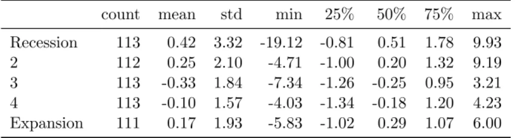
Table XV
Summary Statistics of large cap strategy across five GDP growth regimes. Regime 1 indicates recession and 5 expansion
count mean std min 25% 50% 75% max
Recession 113 0.42 3.32 -19.12 -0.81 0.51 1.78 9.93
2 112 0.25 2.10 -4.71 -1.00 0.20 1.32 9.19
3 113 -0.33 1.84 -7.34 -1.26 -0.25 0.95 3.21 4 113 -0.10 1.57 -4.03 -1.34 -0.18 1.20 4.23 Expansion 111 0.17 1.93 -5.83 -1.02 0.29 1.07 6.00
Can Cashflow Risk Explain the Value Spread?
Keywan Christian Rasekhscha↵e, Francesco Reggiani⇤ June 24, 2013
ABSTRACT
This paper investigates cashflow risk and its relationship to average returns. We find that stocks with earnings that co-vary strongly with market-wide earnings also earn a high return. The cashflow beta (or earnings beta) of value stocks is found to be much higher than that of growth stocks, and small stocks have higher cashflow betas than large stocks. Thus, cashflow betas can explain a significant part of the Fama and French factors. This provides evidence for a risk-based explanation of anomaly returns because stocks earning a higher return also tend to have riskier cashflows. JEL classification: .
I.
Introduction
It is widely known that the classical capital asset pricing model (CAPM) has failed to explain a broad range of anomalies in the closely studied period after 1962. Among the most notable anomalies are the Fama and French (1992) factors, namely size and book-to-market. Adrian and Franzoni (2009) suggest that the beta of value stocks has decreased over time: while the CAPM was able to explain a significant part of the value spread in the beginning of the 20th century, beta becomes negative for the value spread during the latter part of the 20th century. In recent research Frazzini and Pedersen (2010) show that beta not only fails to explain the book-to-market anomaly, but that a spread portfolio formed on beta has a negative expected return. This result calls into question the foundational assumption that riskier assets earn a higher return. From an empirical perspective this also undermines the ability of beta to explain anomalies consistent with theory: Since beta does not have a positive price of risk in the cross-section, it might lack credibility explaining anomalies even if betas are aligned with returns of test assets.
Time-varying aggregate cashflows lead to changes in the investment opportunity set and di-rectly a↵ect current-period wealth. Since listed firms are intertwined with the economy it is not surprising that cashflow shocks correlate positively with changes in gross domestic product (GDP) and consumption. Also, cashflow innovations vary with common indicators of distress such as the default spread and the term-spread. Arbitrage pricing theory suggests that aggregate cashflow (or earnings) risk needs to be priced in the cross-section in order to be a systematic risk factor: stocks whose cashflows are highly sensitive to market-wide cashflow innovations should have high expected returns.
We think that cashflow beta is a very suitable candidate for a risk factor since it inherits much of the theoretical underpinnings of the traditional CAPM. The dividend model of Campbell and Shiller (1988) relates returns to cashflows and therefore firms with riskier cashflows might also be more risky investments. Regardless of whether markets are entirely efficient, it is a widely held belief that riskier assets have higher expected returns. While previous studies (see e.g. Cohen, Polk, and Vuolteenaho (2009); Da and Warachka (2009)) have looked to di↵erent cashflow measures explaining anomalies ex-post, surprisingly little attention has been paid to cashflow beta as a risk factor.
We aim to answer the question: do fundamentally more risky firms earn a higher return. To this end we measure risk by examining the underlying cashflows of firms. Unlike return betas we do not expect cashflow betas to be a↵ected by transitory mispricing. To achieve this we study the cashflow betas of firms and document that cashflow beta-sorted portfolios provide a spread portfolio with positive expected return. To estimate cashflow betas we strictly limit ourselves to information available to investors at any point in time. Each year betas are re-estimated for all stocks and investors learn about cashflow betas only as financial statements become available, which is in contrast to the common approach to estimate betas over the full sample. Estimating betas over the full sample can be especially mis-leading when estimation risk is high which is the case in the present analysis because of the small sample of observations.
The first goal of this paper is to investigate if cashflow beta is priced in the cross-section. To this end we estimate the price of risk of cashflow beta using individual stocks as the test assets. In contrast with traditional beta, we are able to show that cashflow beta has a positive and significant price of risk. To ensure that our estimated price of risk corresponds to an investible strategy, we estimate cashflow betas at all points in time for all stocks. Next, we form portfolios based on the loadings on aggregate cashflow innovations. If the price of cashflow risk is positive, we expect portfolios of assets with high loadings to have high average returns.
We find that cashflow beta carries a significant price of risk. The decile with the highest loading outperforms the decile with the lowest loading by approximately 3.5% per annum. We find this to be consistent with economic theory: low cashflow beta assets e↵ectively provide a hedge against aggregate cashflow shocks and therefore should have a lower price of risk than highly cyclical assets. Furthermore, the dividend model of Campbell and Shiller (1988) shows that cashflows equal returns in the long run. This e↵ectively links cashflow risk to return risk and suggests that high cashflow beta stocks might have high demand and low expected returns because their future returns are expected to be more risky.
The second goal of this paper is to see if returns to book-to-market, size, and long-term mean-reversion portfolios are related to cashflow risk. Since our cashflow risk factor has theoretical underpinnings and has been shown empirically to have a positive price of risk, we now will ana-lyze the cashflow risk of anomaly portfolios. There are reasons to believe that beta-contamination
based anomalies like the book-to-market e↵ect, since these are likely to pick up transitory mispric-ing. Hence cashflow betas are particularly useful in this case since they remain largely una↵ected by temporary inefficiencies. Although cashflow risk of anomaly portfolios has been an area of active research, our measure di↵erentiates itself by having considerable pricing power in the cross-section of stocks and not just anomaly test assets: portfolios of stocks with high ex-ante cashflow loadings have high average returns. Moreover, firm earnings are directly observable and therefore cashflow betas can be directly estimated. Since the beta is not a residual like in the Campbell and Shiller (1988) decomposition, no assumptions about state variables are necessary.
We find that cashflow betas for size and book-to-market portfolios do vary significantly explain-ing a large portion of their returns. High book-to-market portfolios have much higher cashflow betas than low to-market portfolios. In fact the spread in cashflow betas between high book-to-market stocks and low book-book-to-market stocks is almost as large as for cashflow beta sorted portfolios. Also, portfolios with small stocks have higher cash-flow betas than portfolios with large stocks.
Measure
In our analysis we deliberately focus on the simplest cashflow measure possible, year-on-year return on equity innovations, since more complex approaches frequently require assumptions about state variables or make real time estimation impossible. Return on equity innovations are easy to observe, do not require additional assumptions for computation, and we know exactly when the information becomes available. Even though we would like to measure changes in expected cashflows going forward, we limit ourselves to using past cashflow changes in order to provide an empirically sufficient proxy and avoid either relying excessively on specific assumptions of a model or depending on analyst forecasts that are known to be biased. Since we use essentially a backward looking measure we test if sorting on cashflow betas continues to provide a large spread in cashflow-risk loading after portfolio formation. This is particularly important since cashflow beta estimates are not reliable in a statistical sense due to annual data frequency resulting in few data points. We demonstrate that sorting on ex-ante cashflow loadings also produces a large spread in cashflow betas after portfolio formation. Furthermore, book-to-market sorted portfolios and size-sorted portfolios have cashflow betas that are aligned with returns: test assets with higher returns tend to have
riskier cashflows. Provided that cashflow beta is also a priced factor in the cross-section of returns this plausibly suggests that at least some of the observed anomaly returns are due to fundamental risk. Finally, cashflows of book-to-market sorted portfolios are correlated with macroeconomic risk proxies that forecast aggregate returns.
While shareholders ultimately care about the cashflows they receive, earnings are arguably better than net dividends as a proxy for cashflows since dividend payout ratios are driven by many considerations including taxation apart from earnings. Beginning with Ball and Brown (1968) and Beaver (1968), a stream of papers documents that realized stock returns are related to realized earnings, consistent with the casual observation that stock prices move when earnings di↵er from expectation. More recently, Andrew and Johannes (2006) estimate that a disproportionate amount of anticipated stock price volatility is associated with uncertainty resolution around earnings announcements. Thus it appears that expected earnings are at risk; investors “buy” earnings and the return outcome depends on the di↵erence between actual and expected earnings. Also, the large return volatility associated with earnings announcements suggests that investors view current earnings as indicative of future earnings. We measure risk as the cashflow beta coefficient and find that these betas vary systematically with market cashflows and the risk premium.
Literature
It is well known that high book-to-market stocks earn higher returns than low book-to-market stocks. Several studies of dynamic trading strategies suggest that the excess returns of high book-to-market stocks cannot be explained by risk because returns are not explained by the CAPM. Lakonishok, Shleifer, and Vishny (1994) argue that conditional risk models are unlikely to result in a plausible explanation because high book-to-market stocks exhibit a lower beta when returns are negative. They argue that the value premium must be due to overreaction or other behavioral biases. A group of studies endeavours to explain the failure of the unconditional CAPM by introducing conditioning information. Lettau and Ludvigson (2001); Santos and Veronesi (2004); Lustig and Van Nieuwerburgh (2007); Jagannathan and Wang (1996) and Zhang (2005) suggest that betas of book-to-market and size-sorted stocks vary over the business cycle in ways that explain positive unconditional alphas. Petkova and Zhang (2005) find that betas of book-to-market sorted portfolios
argue that the conditional CAPM does not explain the value spread because cross-sectional tests fail to account for restrictions imposed by theory. Beaver, Kettler, and Scholes (1970) suggest that accounting-based risk measures are impounded in market-price-based risk measures. However, recent evidence indicates that accounting-based risk measures may be more successful in explaining the cross section of returns and in particular the value spread. This may result from cashflow betas linking returns to risk, even if some mispricing obscures the link between beta and returns. Risky assets (high book-to-market stocks in most studies) might be underpriced and result in low betas. Brainard et al. (1990) argue that even slight mispricing might contaminate both returns and higher moments. Cohen et al. (2009) show that cashflow betas explain most of the price di↵erence between high and low book-to-market stocks. Nekrasov and Shro↵(2009) also show that cashflow betas reasonably explain the cross section of average returns. In related research Campbell and Vuolteenaho (2004) decompose beta into a cashflow and discount rate component and show that high book-to-market stocks have relatively high cashflow betas and low discount-rate betas. They argue that cashflow betas should carry a higher risk premium. Cohen et al. (2009) conclude that return betas approach cashflow risk as the holding period increases. Da and Warachka (2009) show that systemic earnings forecast revisions are a useful predictor of cross-sectional anomalies.
Since many characteristics may align with anomaly portfolio returns (Lewellen and Nagel (2006)), it is important that proposed risk factors have power not only in the cross section of anomaly portfolios, but also individual equities. Thus our study adds to previous research like Cohen et al. (2009) and Da and Warachka (2009) because it does not merely focus on cashflow risk after portfolio formation without linking the cashflow measure to the cross-section of anomaly factor returns.
II.
Methodology
Cashflow risk motivation
Since stock prices equal the discounted sum of future cashflows, stock returns are naturally driven by earnings realizations. Campbell and Shiller (1988) decompose stock returns in a cashflow component (NCF,t+1) and a discount rate component (NDR,t+1):
rt+1 Et[rt+1] =NCF,t+1 NDR,t+1 (1)
where the discount rate component equals
NDR,t+1 = (Et+1 Et) 1
X
j=1
⇢jrt+j+1 (2)
and the cashflow component equals
NCF,t+1= (Et+1 Et) 1
X
j=1
⇢jdt+j+1 (3)
where dt+j+1 and rt+j+1 denote, respectively, the log stock cashflow growth and the log stock return over a future time period [t+j, t+j+1) with⇢being the log-linearization constant (commonly set to 0.95 with annual frequency). Cashflows from Equation (3) do not equal changes in expected earnings since cashflows represent outflows from the firm to the investor. Earnings represent an inflow of funds. Earnings and cashflows from Equation (3) are related through the clean surplus accounting identity:
Bt+1 =Bt+Xt+1 Dt+1 (4)
where Bt+1 is book equity, Xt+1 is earnings, and Dt+1 is cashflows. dt+j+1 from Equation (3) is the log ofDt+j+1. The log return on book equity is:
et+j+1 =log(1 + ✓ Xt+j+1 Bt+j ◆ ) (5)
Campbell and Vuolteenaho (2004) and Cohen et al. (2009) log-linearize the clean surplus identity and replace cashflows dt+j+1 in Equation (3) with log returns on book equity. Thus the cashflow component becomes: NCF,t+1 = (Et+1 Et) 1 X j=1 ⇢jet+j+1 (6)
cashflows to shareholders eventually need to be financed by earnings.
For our purposes it is more natural to examine earnings rather than cashflows since dividends are known to be smoothed and dividend policy is also impacted by many considerations apart from expected cashflow shocks (i.e. tax treatment). Since cashflows eventually need to be paid from earnings, current earnings shocks might be a better proxy than current cashflow shocks for future cashflow shocks.
Cashflow risk measure
Equation (6) suggests that the cashflow component of stock prices requires the knowledge of cashflow shocks across all horizons. However, in our analysis we rely on past cashflow shocks since future expected shocks are not directly observable. Several papers from the accounting litera-ture (see e.g.: Ball and Brown (1968) and Beaver (1968),) document that price changes correlate highly with earnings changes. In a more recent study Andrew and Johannes (2006) estimate that a disproportionate amount of anticipated stock price volatility is associated with uncertainty resolu-tion around earnings announcements, which suggests that current earnings shocks inform investors about future earnings shocks.
Specifically, our cashflow proxy for Equation (3) is defined as follows:
NCF,t = et Bt 1
(7) To construct market-wide earnings innovations we take the cross-sectional sum of etfor each year and divide it by the cross-sections mean ofBteach year where etare earnings innovations at time tand Bt 1 is book value at timet 1.
Pre-formation regressions
Our goal is to to test whether stocks with di↵erent sensitivities to market-wide earnings innova-tions have di↵erent average returns. To measure the sensitivity to market-wide earnings innovations we first compute expanding window regressions for each stock with sufficient observations:
where i and M superscripts denote portfolios and the market respectively. The cashflow beta i
CF,t 1 denotes the co-variance between changes in portfolio earning and changes in market-wide earnings at time t 1. We re-estimate CF,ti 1 each year in order ensure all information is in the investor’s information set.
We construct a set of test assets that are diverse in their cashflow beta by sorting firms into portfolios each calendar year based on their latest CF,ti 1 . We use all stocks from AMEX, NAS-DAQ and NYSE that have a minimum of ten observations in order to make estimates reasonably precise. We then hold the portfolios constant and measure their returns from June in year t to June in year t+ 1 to ensure the inputs for Equation (8) were known to investors.
Estimation of cashflow betas of test assets
For our estimation of cashflow betas of anomaly portfolios, we aggregate firm-level earnings innovations from Equation (7), and regress portfolio earnings innovations on market earnings in-novations.
NCF,t=↵iCF + CF,ti NCF,tM +"it (9)
Cross-sectional regressions
Our cross-sectional regressions involving individual stocks and the 20 size and book-to-market portfolios confirm the economic intuition that cashflow betas should be a priced risk factor. We take the regression coefficients CF,ti 1 from Equation (8) and estimate the following cross-sectional regression:
rti+ rft= 0+ 1 CF,ti 1+"it+ (10) where the dependent variable ri
t+ represents the returns to portfolio i, and rft represents the risk-free rate over the same horizon.
III.
Empirical results
DataOur data is from the Compustat annual file and the Center for Research in Security Prices database (CRSP), and covers the 1962-2010 period. All firms are listed in the United States, and we exclude all firms that do not have their fiscal-year-end in December to ensure contemporaneous cashflows. We use book value of common equity and earnings before extraordinary items from Compustat. Stock prices and returns are from CRSP. Price per share is taken at fiscal-year-end and book value and earnings are assumed to be known six months after. Book value is computed as Compustat common equity (CEQ) plus preferred treasury stock (TSTKP), less preferred dividends in arrears (DVPA). Earnings is defined as earnings before extraordinary items (IB), less special items (SPI), adjusted for taxes.
Firm-year observations with negative book value, missing earnings, or share price less than 20 cents are excluded from the analysis. Also, firms missing shares outstanding are excluded. Other missing data items are set to zero. The variables used to fit the expected risk premium are defined as follows: the dividend yield is the sum of dividends accruing to the CRSP value-weighted index of the trailing twelve months divided by the level of the index. The default spread is the yield spread between Moody’s Baa and Aaa corporate bonds. The term premium is the spread between the ten-year and the one-year treasury bond. Default yields are from the monthly database of the Federal Reserve Bank of St. Louis. Government bond yields are from the Ibbotson database, and the short rate is the one month treasury bill rate from CRSP.
Summary statistics
There are 68,716 firm-years in the investigation over our 44 year period, with an average of 1,561 firms per year. Panel A of Table I gives the distribution of monthly returns from the 12 months over which they are observed and distributions of the estimated book-to-market (B/M) and return on common equity (ROCE). The table description explains the trimming of variables for the means and standard deviations. The table reports that the distributions of returns and B/M in the sample are quite similar to those for all firms on CRSP and Compustat. The relationship between B/M and other variables is highlighted in Panel B of Table I where characteristics of five
portfolios formed from ranking firms on B/M are reported. As in Fama and French (1992) among others B/M is positively correlated with returns over the subsequent 12 months, suggesting that high B/M stocks require a higher return. Note that B/M is negatively correlated with ROCE, and high B/M firms have lower profitability and are identified with higher risk in asset pricing models.
[Place Table I about here]
Cashflow beta sorted portfolios: Post-formation factor loadings
In the penultimate row of Table II, we present the post-formation factor loadings of the cashflow beta sorted portfolios. We computed them as follows: After forming portfolios by sorting on cashflow beta estimates available at timet, we sum all earnings innovations and book values in the following year t+ 1 for each portfolio and compute the portfolio cashflow beta by regressing on market cashflow innovations as described with Equation (9).
The penultimate row in Table II indicates that portfolios formed on past i
CF show a significant spread in i
CF over the subsequent year.
Cashflow beta sorted portfolios: Post-formation returns
The first row of Table II presents port