Multiple Adaptive Mechanisms for Data-driven Soft Sensors.

Multiple Adaptive Mechanisms for Data-driven Soft Sensors

Rashid Bakirov∗, Bogdan Gabrys, Damien Fay

Data Science Institute, Bournemouth University Fern Barrow, Poole House P256, Talbot House

BH12 5BB Poole, UK

Abstract

Recent data-driven soft sensors often use multiple adaptive mechanisms to cope with non-stationary environments. These mechanisms are usually deployed in a prescribed order which does not change. In this work we use real world data from the process industry to compare deploying adaptive mechanisms in a fixed manner to deploying them in a flexible way, which results in varying adaptation sequences. We demonstrate that flexible deployment of available adaptive methods coupled with techniques such as cross-validatory selection and retrospective model correction, can benefit the predictive accuracy over time. As a vehicle for this study, we use a soft-sensor for batch processes based on an adaptive ensemble method which employs several adaptive mechanisms to react to the changes in data.

Keywords:

Soft sensors, Adaptive mechanisms, Streaming data, Ensemble methods

1. Introduction

Modelling industrial processes typically involves estimating a finite set of physical quantities. Certain necessary measurements in the process industry are often excessively costly or time consuming. Soft sensors have proven to be useful tools in these situations, providing information about the quantity to be estimated without directly performing the measurements. There are two main families of soft sensors; physical model based and data-driven soft sensors [1]. Physical model-driven soft sensors estimate the quantity using chemical and physical laws behind the process. For many complex processes this is impossible as accurate first principle models are not known or evolution of the process is not taken into account.

In this work we focus on data-driven soft sensors. In particular we scrutinise and explore the multiple adaptive mechanisms applied to soft sensors in a streaming data sce-nario. The streaming data scenario itself introduces some interesting questions. For the

∗_{Corresponding author}

Email addresses: [email protected](Rashid Bakirov),[email protected]

(Bogdan Gabrys),[email protected](Damien Fay)

batch processes where data arrives in large segments called batches, which are common in the process industry, especially in the chemical, microelectronics and pharmaceutical areas [2], the models are typically adapted when a new batch of data is observed. This can be done with or without historical data (which may have been jettisoned, is not readily available or would be computationally costly to include).

The underlying assumptions of a soft-sensor model may only hold for a certain period of time [3]. It has been shown that many changes in the environment which are no longer being reflected in the model contribute to the deterioration of predictive model’s accuracy over time [4, 5]. Factors such as sensor/measurement deterioration, addition of new sensors, changes in the process flow or input materials etc. can result in alternate models explaining the process better. This requires constant manual retraining and readjustment of the soft sensors which is often expensive, time consuming and in some cases impossible - for example when the historical data is not available any more.

To avoid outright retraining and development of soft-sensor models for an evolving process, many soft sensors with adaptive mechanisms (AMs) [5] have been proposed, starting with the recursive Principal Component Analysis (PCA) and Partial Least Squares (PLS) approaches presented in [6, 7] and developing as discussed later (Sec-tion 2). Often adapta(Sec-tion operates by reducing the weight applied to irrelevant parts of the historical data, which may be implemented in a variety of ways. In addition, recent adaptive soft sensors use, not one, but multiple AMs. Employing multiple AMs is more versatile than a single approach and can lead to superior prediction performance (e.g. [8, 9]) because given an evolution in the process some AMs are more appropriate than others at different times. However, in practice, most research has concentrated on AM’s deployed in a prescribed fixed order set at the model design time. The common choice is to deploy all of the AMs at the same time, however this can lead to undesirable results with some AMs cancelling the effect of others or by overcompensating for change in the process.

In this paper we are providing a deeper analysis of a soft sensor with multiple AMs, concentrating on the choice and order of AMs’ deployment. For this purpose we use the Simple Adaptive Batch Learning Ensemble (SABLE) [10], on which the analysed soft sensor is based. SABLE is an ensemble method, meaning that the final prediction is cal-culated by combining the predictions of different models (experts). As such, it uses three different popular AMs to deal with changing data; (i) Recursive Partial Least Squares (RPLS) [11] is used to discount older data, (ii) adapting the combination weights targets the ensemble mix, and (iii) addition/merge/removal of experts adapts the structure of the model ensemble. This allows us to relate to many other soft-sensors which use sim-ilar AMs for their adaptation, making our exploration relevant to a very broad class of similar approaches.

As a result of our analysis based on three real world process industry datasets we provide strong empirical evidence that deploying AM’s in a flexible order without a predetermined sequence leads to better prediction accuracy. Two methods in particular were effective for the choice of the AM - cross-validatory selection and retrospective model correction (see Section 3.2). Cross-validatory AM selection involves selecting the AM to deploy based on the performance on the current data. Once the subsequent data has been fully observed, the AM which would indeed have been the best for previous batch becomes known. Retrospective model correction is reverting the model to the state, which the deployment of this best AM would have created.

The paper is structured as follows; Section 2 introduces the related work, concentrat-ing on soft sensors with one or more adaptive mechanisms. Section 3 presents mathemat-ical formulation of the framework of a system with multiple adaptive elements in batch streaming scenario. Section 4 introduces the algorithm for the soft-sensor, which was used for the experimentation, including its AMs and a description of RPLS. Experimen-tal methodology, description of the datasets and results of our experiments are covered in Section 5. We conclude by giving our final remarks in Section 6.

2. Related Work

Recently, many soft sensors and other regression methods for industrial processes, which explicitly consider the adaptation of the model, such as [8, 9, 12–24], have been proposed. Many of the algorithms are examples of incremental learning, with the excep-tion of [9, 21] which are specifically targeted at batch processes. Adaptivity is usually achieved by building a predictive model using a) the latest historical data; and/or b) the historical data which is the most similar to the current data. Adaptive methods often use multiple models to make the final prediction, either by the weighted combination of their outputs[8, 9, 12–17, 21, 22, 24] - these are known as ensemble models, or, more rarely, selecting one of them [18, 21, 23]. Most of the models, or experts, are built on the subsets of historical data which represent different degrees of relation to the current data.

Ensemble methods date as far back as 1960s, when it was shown that combining multiple predictive models may give better results than using single models [25]. One of the advantages of ensemble methods is the ability to model local dependencies in the data, a classical example being an adaptive mixture of local experts presented in [26]. This is achieved by weighting the models’ predictions on a data instance by the location of this instance in the input space. Soft sensors using local ensembles are described in [8, 9, 22, 24, 27, 28]. These methods first identify the disjoint segments of the historical input space where the process produced outputs described by a common model, sometimes also calledreceptive fields. Then they build a model for each receptive field using Partial Least Squares (PLS) [29] or Support Vector Regression [30]. The models therefore describe different regions of the process. The final prediction is a weighted average of all of the experts. Here, for each new data instance, the weights of experts depend on the location of the observed instance and in some cases the prediction. The AM used in [27] is based on change of models’ local weights depending on their error. This model was extended in [8] to include adaptation of the base models using the RPLS forgetting. [28] further extends the model to include creation of additional experts. [22, 24] uses adaptation of base models and adaptive weighting with [9] additionally introducing adaptive offset correction. Another soft sensor based on local ensemble with a moving window and weights change AMs is described in [12].

Also popular in the literature are global regression ensembles [13–16]. These typically assign weights to experts based on their general performance, not considering the local aspects of data. Global ensemble methods use similar AMs. For instance, [13] adapts to changes by creating new experts and changing their weights. [16] includes AMs such as adaptation of base models via a moving window strategy, changing experts weights and adding new experts. [15] additionally employs a boosting like instance weighting mechanism resampling the training data. Both [15] and [16] may remove experts as well.

A method which uses an ensemble of univariate regressors for multivariate regression is described in [17]. It includes weighting of models and forgetting factor AMs. [31] uses time differenceensemble based on the distance between the current input and historical inputs. This method can use either moving window or just-in-time (creation of a model from most relevant instances) approaches for adaptation. [31] also uses just-in-time model creation with global performance based adaptive weighting.

From the analysis above we can see that there are a host of adaptation mechanisms which can be applied with ensemble methods. A review of these mechanisms for soft sensors is given in [5]. The mechanisms target different characteristics of the model; the error, the current location in the input space (or output space), and the temporal distance. The SABLE framework chosen here also includes such functionality. Most of the described work above have a common characteristic that whatever the AMs, they are applied at every time step in the same manner. In contrast the approaches proposed in [15, 16, 21, 28, 31, 32] change the order of the adaptation. This research is perhaps the most relevant to the current paper. In particular, [28] creates new experts when existing ones are not built on the relevant data, [15, 16] create new experts when the predictive error on an instance is above a set threshold. In [31] the predictive accuracy is assessed to switch between two predictive models. Again the, predictive accuracy is used to choose between just-in-time model creation and offset update in [21]. [32] presents a plug and play architecture for preprocessing, adaptation and prediction which foresees the possibility of using different adaptation methods in a modular fashion, but does not address the method of AM selection. The research presented here differs from the existing studies as, to the best of authors’ knowledge, it is the first work to examine how changing the order and the type of adaptation affects the system characteristics and performance.

3. Formulation

We assume that the data is generated by an unknown time varying process which can be formulated as:

yτ =ψ(xτ, τ) +τ, (1)

where ψ is the unknown function, τ a noise term, x∈ RM is an input data instance, andyτ is the observed output at timeτ12. Then we consider the predictive method at a timeτ as a function:

ˆ

yτ =fτ(xτ,Θf), (2)

where ˆyτ is the prediction,fτ is an approximation (i.e. the model) ofψ(x, τ), and Θf is the associated parameter set. Our estimate,fτ, evolves via adaptation as each batch of data arrives as is now explained.

1_{Please note that Equation 1 has not intended to and do not explicitly take into account the dynamics}

of the data generating process as is commonly done in the state-space model representation used in the

control engineering. Herex represents all measurable/observable variables (e.g. sensor readings, etc.)

which are used as inputs to the prediction model as expressed in Equation 2.

2_{The notation used in this paper is listed in the Table A.6}

𝐺

𝑓

𝒚

𝑓

𝒚

̂

𝑓

−

𝑿

𝑔

𝑔

Figure 1: Adaptation with multiple AMs. Optional inputs are shown with dashed lines.

3.1. Adaptation

In the batch streaming scenario considered in this paper, data arrives in batches with τ∈ {τk· · ·τk+1−1}, where τk is the start time of the k-th batch. If nk is the size of thek-th batch, τk+1 =τk +nk. It then becomes more convenient to index the model by the batch numberk, denoting the inputs asXk =xτk,· · ·,xτk+1−1, the outputs as

yk =yτk,· · · , yτk+1−1. We examine the case where the prediction functionfk is static

within ak-th batch.3_.

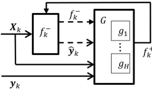
We denote the a priori predictive function at batch k as f_k−, and the a posteriori predictive function, i.e. the adapted function given the observed output, as f_k+. An adaptive mechanism,g(·), may thus formally be defined as an operator which generates an updated prediction function based on the batchVk ={Xk,yk} and other optional inputs. This can be written as:

gk(Xk,yk,Θg, fk−,yˆk) :f

−

k →f

+

k. (3)

or alternatively asf_k+=f_k−◦gk for conciseness. Notefk−and ˆyk are optional arguments and Θg is the set of parameters ofg. The function is propagated into the next batch as f_k+1− =f_k+ and predictions themselves are always made using thea priori functionf_k−.

We examine a situation when a choice of multiple, different AMs,

{∅, g1, ..., gH}=G, is available. Any AM ghk ⊂ G can be deployed on each batch,

wherehk denotes the AM deployed at batchk. As the history of all adaptations up to the current batch, k, have in essence created f_k−, we call that sequence gh1, ..., ghk an

adaptation sequence. Note that we also include the option of applying no adaptation denoted by ∅. In this formulation, only one element of G is applied for each batch of data. Deploying multiple adaptation mechanisms on the same batch are accounted for with their own symbol inG. Figure 1 illustrates our formulation of adaptation.

3.2. Adaptation strategies

In this section we present the different strategies we examined to understand the issues surrounding flexible deployment of AMs better and assist in the choice of adaptation sequence.

3_{A batch typically represents a real-world segmentation of the data which is meaningful, for example}

a plant run and so our adaptation attempts to track run to run changes in the process. We also found in our experiments that adapting within a batch can be detrimental as its leads to drift in the models.

At every batchk, an AMghk must be chosen to deploy on the current batch of data.

To obtain a benchmark performance, we use agreedy optimal adaptation strategy f_k+1− =f_k−◦ghk, hk= argmin

hk∈1···H

h(f_k−◦ghk)(Xk+1),yk+1i (4)

where h i denotes the chosen error measure4_{. Since X}

k+1,yk+1 are not yet obtained, this strategy is not applicable in the real life situations. Also note that this may not be the overall optimal strategy which minimizes the error over the whole dataset. While discussing the results in the Section 5 we refer to this strategy asOptimal.

Given the inability to conduct the Optimal strategy, below we list the alternatives. The simplest adaptation strategy is applying the same AM to every batch (these are denotedSequence1,Sequence2etc. in Section 5). A more common practice (see Section 2) is applyingall adaptive mechanisms, denoted asJoint in Section 5.

As introduced in [10], it is also possible to use Vk for the choice of ghk. Given the

observation, thea posteriori prediction errorVk ish(fk−◦ghk)(Xk),yki. However, this is effectively an in-sample error asghk is a function of{Xk,yk}.

5 _{To obtain a generalised} estimate of the prediction error we apply 10-fold cross validation. The cross-validatory adaptation strategy (denoted asXVSelect) uses a subset (fold),S, of{Xk,yk}to adapt; i.e. f_k+ = f_k− ◦ghk({Xk,yk}∈S) and the remainder, S, is used to evaluate, i.e. find

hf_k+(Xk)_∈ S,yk ∈ S

i. This is repeated 10 times resulting in 10 different error values and the AM,ghk ∈G, with the lowest average error measure is chosen. In summary:

f_k+1− =f_k−◦ghk, hk= argmin

hk∈1···H

h(f_k−◦ghk)(Xk),yki× (5)

whereh i× _{denotes the cross validated error.}

The next strategy can be used in combination with any of the above strategies as it focuses on the history of the adaptation sequence and retrospectively adapts two steps back. This is called the retrospective model correction [33]. Specifically, we estimate which adaptation at batchk−1 would have produced an optimal estimate in blockk:

f_k+1− =f_k−₋₁◦ghk−1◦ghk, hk−1= argmin

hk−1∈1···H

h(f_k−₋₁◦ghk−1)(Xk),yki (6)

Using cross-validated error measure in Equation 6 is not necessary, because ghk−1 is

independent ofy_k. Also note the presence of ghk; retrospective correction does not in

itself produce a fk+1 and so cannot be used for prediction unless it is combined with another strategy (ghk). This strategy can be extended to consider the sequence ofrAMs

while choosing the optimal state for the current batch, which we callr-step retrospective correction:

f_k+1− =f_k−_−r◦ghk−r◦ · · · ◦ghk−1◦ghk, {hk−r· · ·hk−1}= argmin

hk−r···hk−1∈1···H

h(f_k−_−r◦ghk−r◦ · · · ◦ghk−1)(Xk),yki (7)

4_{In this paper Mean Absolute Error (MAE) is used.}

5_{As a solid example consider the case wheref}+

k isf

−

k retrained using{Xk,yk}. In this caseykare

part of the training set and so we risk overfitting the model if we also evaluate the goodness of fit onyk.

X

P

T

U

Q

B

...

P

T

U

Q

B

...

P

T

U

Q

B

...

P

T

U

Q

B

...

P

T

U

Q

B

...

P

T

U

Q

B

...

P

T

U

Q

B

...

P

T

U

Q

B

...

D

Σ

P

T

U

Q

B

...

P

T

U

Q

B

...

P

T

U

Q

B

...

P

T

U

Q

B

...

P

T

U

Q

B

...

P

T

U

Q

B

...

P

T

U

Q

B

...

P

T

U

Q

B

...

D

P

T

U

Q

B

...

P

T

U

Q

B

...

P

T

U

Q

B

...

P

T

U

Q

B

...

P

T

U

Q

B

...

P

T

U

Q

B

...

P

T

U

Q

B

...

P

T

U

Q

B

...

D

P

T

U

Q

B

...

P

T

U

Q

B

...

P

T

U

Q

B

...

P

T

U

Q

B

...

P

T

U

Q

B

...

P

T

U

Q

B

...

P

T

U

Q

B

...

P

T

U

Q

B

...

D

y

^

[ ]

[ ]

[ ]

[ ]

y

^

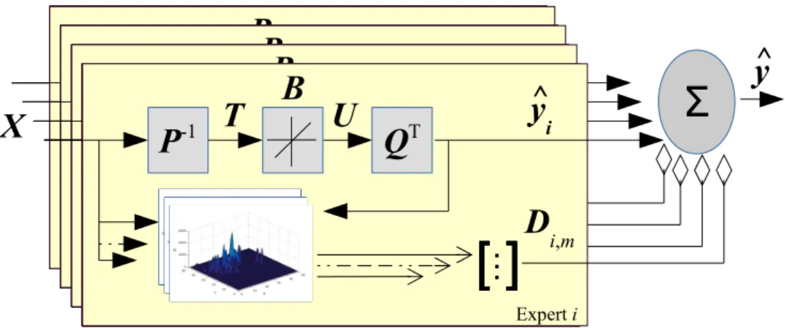
Figure 2: Block diagram of SABLE model.

We next examine the prediction algorithm and the adaptive mechanisms (the setG) used in this research.

4. Algorithm

To perform experiments, we chose a modelling framework which has the ability to implement several different types of adaptation mechanisms. This is called the Simple Adaptive Batch Local Ensemble (SABLE)6_{, which is an extension of the ILLSA method} [8]. ILLSA uses an ensemble of models, called base learners, with each base learner implemented using a linear model formed through RPLS. TO get the final prediction, the predictions of base learners are combined using input/output space dependent weights (i.e. local learning). SABLE differs from ILLSA in that it is designed for batches of data whereas ILLSA works and adapts on the basis of individual data points. Furthermore, SABLE supports the creation and merger of base learners. PLS was chosen because it is widely used for predictions in chemical processes where high dimensional datasets tend to have low-dimensional embeddings. Figure 2 shows the diagram of SABLE model . 4.1. Building of Experts’ Descriptors

The relative (to each other) performance of experts varies in different parts of the input/output space. In order to quantify this adescriptor is used. Descriptors of experts are distributions of their weights with the aim to describe the area of expertise of the particular local expert. They describe the mappings from a particular input, xm_{, and} output,y, to a weight, denotedDi,m(xm, y), wheremis themthinput feature7 andiis

6_{SABLE was previously described in [10], Sections 4, 5, 6. To make this work self contained, we}

repeat the description of the algorithm again in this Section.

7_{For the base methods which transform the input space, such as PLS, the transformed input}

argu-ments are used instead of original ones.

thei-th expert. The descriptor is constructed using a two-dimensional Parzen window method [34] as: Di,m = 1 ||Vtri || ||Vtr i || X j=1 w(xj)Φ(µmj ,Σ) (8)

whereVtri is the training data used for ith expert, ||V tr

i || is the number of instances it includes,w(xj) is the weight of sample point’s contribution which is defined below,xj is the jth sample of Vtri , Φ(µmj ,Σ) is two-dimensional Gaussian kernel function with mean valueµ= (xm

j , yj) and variance matrix Σ∈ <2×2 with the kernel width,σ, at the diagonal positions. σ, is unknown and must be estimated as a hyperparameter of the overall algorithm8_.

The weightsw(xj) for the construction of the descriptors (see Eq. 8) are proportional to the prediction error of the respective local expert:

w(xj) = exp(−(ˆyj−yj)2) (9)

Finally, considering that there are M input variables and I models, the descriptors may be represented by a matrix,D∈ <M×I _{called thedescriptor matrix.}

4.2. Combination of Experts’ Predictions

During the run-time phase, SABLE must make a prediction of the target variable given a batch of new data samples. This is done using a set of trained local expertsF

and descriptors V. Each expert makes a prediction ˆyi for a data instance x. The final prediction ˆy is the weighted sum of the local experts’ predictions:

ˆ y= I X i=1 vi(x,yˆi)ˆyi (10)

wherevi(x,yˆi) is the weight of thei-th local expert’s prediction. The weights are calcu-lated using the descriptors, which estimate the performance of the experts in the different regions of the input space. This can be expressed as the posterior probability of thei-th expert given the test samplexand the local expert prediction ˆyi:

vi(x,yˆi) =p(i|x,yˆi) =

p(x,yˆi|i)p(i) ΣI

j=1p(x,yˆj|j)p(j)

, (11)

wherep(i) is thea priori probability of thei-th expert9_{, Σ}I

j=1p(x,yˆj)p(j) is a normalisa-tion factor andp(x,yˆi|i) is the likelihood ofxgiven the expert, which can be calculated by reading the descriptors at the positions defined by the samplexand prediction ˆyi:

p(x,yˆi|i) = M Y m=1 p(xm,yˆi|i) = M Y m=1 Di,m(xm,yˆi). (12)

8_{In this research the inputs are first divided by their standard deviation so allowing us to assume an}

isotropic kernel for simplicity and also to reduce the number of parameters to be estimated.

9_{Equal for all local experts in our implementation, different values could be used for experts’}

priori-tization.

Eq. 12 shows that the descriptorsDmare sampled at the position which are given on one hand by the scalar valuexm_{of them-th feature of the sample pointxand on the other} hand by the predicted output ˆyi of the local expert corresponding to the ith receptive field. Sampling the descriptors at the positions of the predicted outputs may result in different outcome than sampling at the positions of correct target values, because the predictions are not necessarily similar to the correct values. However the correct target values are not available at the time of the prediction. The rationale for this approach is that the local expert is likely to be more accurate if it generates a prediction which conforms with an area occupied by a large number of true values during the training phase.

To reduce the number of redundant experts, after the processing of batchk, those that deliver similar predictions onVk can be merged, making use of the linear base model. If the base model is not linear and merging is not straightforward, then a pruning strategy as in [27] can be considered. There, the weight vectors of all experts on a batch of data are pairwise compared and if their similarity is higher than the defined threshold, one of the experts is removed. Prediction vectors can also be used to measure the similarity between different experts.

4.3. Adaptive Mechanisms

The SABLE algorithm allows the use of different adaptive mechanisms. AMs are deployed as soon as the true values for the batch are available and before predicting on the next batch. It is also possible that none of them are deployed. The AMs that are used in our work are described in the following sections.

4.3.1. Batch Learning

The simplest AM augments existing data with the data from the new batch and retrains the model. Given predictions of each expert fi ∈ F on V, {yˆ1, ...,yˆI} and measurements of the actual values, y, V is partitioned into subsets in the following fashion:

z=argmin

i∈1···I

hfi(xj), yji → [xj, yj]∈Vz (13)

for every instance [xj, yj]∈V. This creates subsetsVi, i= 1...I such that∪Ii=1Vi=V. Then each expert is updated using the respective dataset Vi. This process updates experts only with the instances where they achieve the most accurate predictions, thus encouraging the specialisation of experts and ensuring that a single data instance is not used in the training data of multiple experts. This AM will be denoted as AM1 in the description of the experiments below.

4.3.2. Batch Learning With Forgetting

This AM is similar to one described in Section 4.3.1 but includes a forgetting factor (see Section 4.4) which reduces the weight of the experts historical training data, making the most recent data more important. This AM will be denoted as AM2.

4.3.3. Recalculation of Descriptors

This AM recalculates the local descriptors, D, using the new batch as described in the Section 4.1. The previous weights are discarded. This AM will be denoted as AM3.

(a) Initial state

AM4

AM2

AM3

(b)

(c)

(d)

Adding new expert and recalculating descriptors i.e. changing combination weights. Retraining of both models with forgetting. Recalculating descriptors.

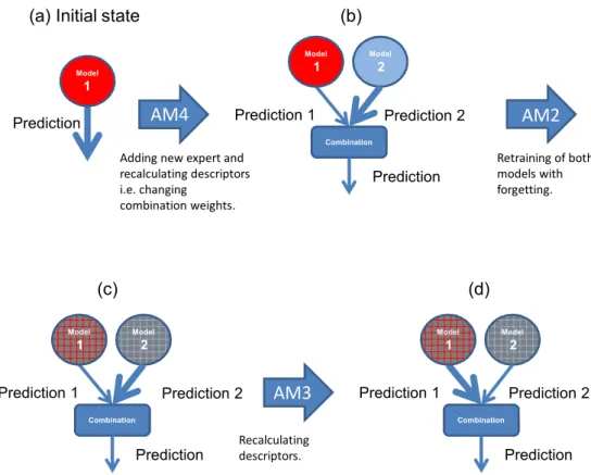
Figure 3: An example of a model adaptation sequence using SABLE AMs

4.3.4. Creation of New Experts

New expert fnew is created from Vk. Then it is checked if any of the experts from

Fk−1∪fnew, where Fk−1 is the experts pool after processing of batch k−1, can be merged or pruned. Finally the descriptors of all resulting experts are calculated (Section 4.1). This AM will be denoted as AM4.

An example of the general principle of SABLE’s operation including few selected adaptation mechanisms is illustrated in the Figure 3. It shows how the model changes after deploying AM4, AM2 and AM3 in a sequence.

4.4. Recursive Partial Least Squares

SABLE is conceived as an algorithm which can function with any base prediction model, assuming the feature independence. In our experiments we use RPLS as a base algorithm. The advantages of this algorithm are that it derives a set of independent latent variables (features) which can be fed into the SABLE instead the original ones, acting as a pre-processing step. Furthermore RPLS can be updated without requiring the historical data and the merging of two models can be easily realised. RPLS is an extension of the Partial Least Squares, both being popular in chemical process modelling. PLS projects the scaled and mean centered multidimensional input data X ∈ RN×M

and output dataY ∈ RN×C_{, whereN is the number of data instances,M is the number} of input variables andC is the number of output variables, to separate latent variables,

X=T ST +E (14)

Y =U QT +F. (15) HereT ∈ RN×L _{(L≤M as the number of latent variables) andU ∈ R}N×L _{are the} score matrices,S ∈ RM×L _{andQ∈ R}C×L _{are the corresponding loading matrices, and}

E and F are the input and output data residuals. Then the score matrices T and U

consist of so called latent vectors:

T = [t1, ...,tL], wheretl∈ Rn×1, l∈1· · ·L (16)

U = [u1, ...,uL], whereul∈ Rn×1, l∈1· · ·L. (17) where the column vectorss ∈ Rm×1 _{and q ∈ R}m×1 _{of the loading matricesS and Q} represent the contributions of the input and output variables to the mutually orthonormal latent vectorstandu, respectively. Equations 16 and 17 constitute the PLS outer model. Afterwards a regression model, which is also called the PLS inner model, between the latent scores is constructed:

U =T B+R, (18) whereB∈ Rl×l_{is a diagonal matrix of regression weights which minimizes the regression} residualsR. Then the estimates ˆY ofY are:

ˆ

Y =T BQT, (19) There are different methods to calculate the required vectors t, s, u, q and b(column vector ofB). One of the most popular ones, NIPALS [35], updates latent vectors in an iterative way. After each iteration, the explained covariance is removed from the data:

Xi+1=Xi−tisTi (20)

Yi+1=Yi−uiqTi . (21) The subsequent (i+ 1)-th vectors are calculated by the resulting new input and output data Xi+1 and Yi+1. Recursive PLS, which uses NIPALS, updates the matrices S,

T, Q, U and B when the new data becomes available, on either sample-by-sample (incremental) or batch basis. In this work we are using batch adaptation. It works by applying PLS on the new batch and constructs new input and output matrices as follows:

Xnew= λST₀ ST₁ (22) Ynew= λB0QT0 B1QT1 , (23)

where the matrices S0, B0 and Q0 describe the old model and S1, B1 and Q1 the new one created from the most recent batch. 0≤λ≤1 is the forgetting factor which

determines how much influence the historic data will have, with λ = 0 meaning zero influence andλ= 1 meaning that the historical data has the same influence as the new batch. After constructing the new input and output data matrices, PLS is applied on them to get the updated matrices. The condition for this update is that the number of latent variables must be equal to the rank ofX. This condition can be practically met by finding a number of latent variablesafor which the error on the training data is less than the defined threshold close to 0.

5. Experimental results

5.1. Methodology

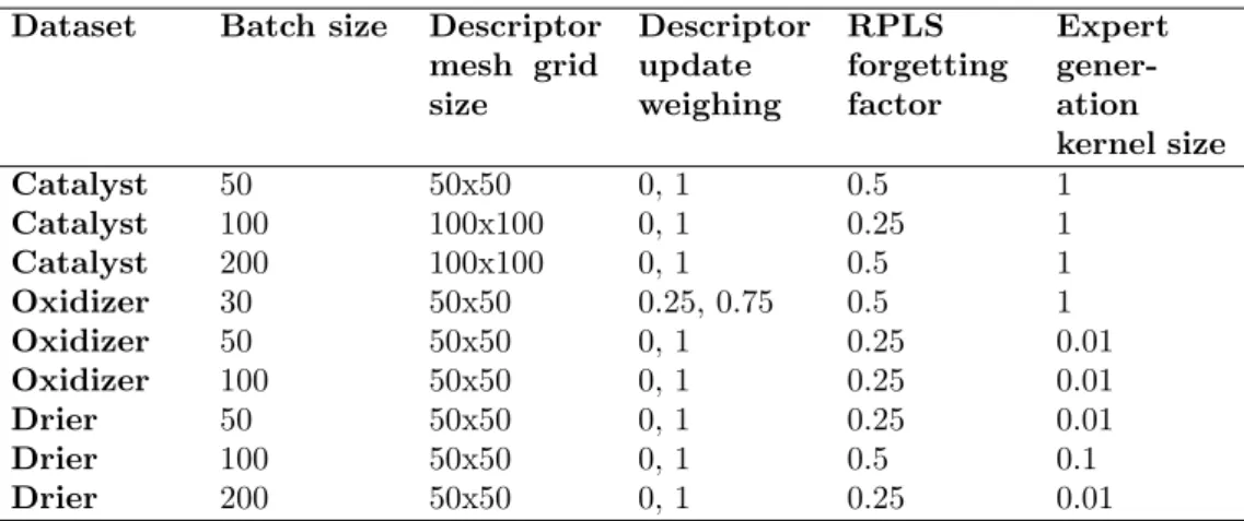
The experiments were performed on 3 datasets from the process industry which will be described later10_{. As explained in [32], there is a need for adaptation for the Oxidizer} and particularly for the Catalyst datasets, which is not apparent with the Drier dataset. We have performed our experiments on all of the three datasets with different batch sizes. Choosing these datasets will allow us to test AM sequences on data which exhibit different behaviours. Three different batch sizes for each dataset are examined in the simulations together with a mix of typical parameter settings as tabulated in Table 1 (for brevity purposes we will denote the batch size next to the dataset name in the future, to indicate which batch size was used for the experiment - i.e. Catalyst50 stands for Catalyst dataset with batch size of 50). These parameter combinations were empirically identified. We use the adaptive strategies presented in Table 2 for AM selection.

Dataset Batch size Descriptor mesh grid size Descriptor update weighing RPLS forgetting factor Expert gener-ation kernel size Catalyst 50 50x50 0, 1 0.5 1 Catalyst 100 100x100 0, 1 0.25 1 Catalyst 200 100x100 0, 1 0.5 1 Oxidizer 30 50x50 0.25, 0.75 0.5 1 Oxidizer 50 50x50 0, 1 0.25 0.01 Oxidizer 100 50x50 0, 1 0.25 0.01 Drier 50 50x50 0, 1 0.25 0.01 Drier 100 50x50 0, 1 0.5 0.1 Drier 200 50x50 0, 1 0.25 0.01

Table 1: SABLE parameters for different datasets

To calculate the significance of differences between the predictions of different strate-gies, the significance test of difference of two estimators’ errors relying on the sample covariance ([36], Section 3.2) was used.

10_{This Section is a partial repeat of the Section 7 from [10]}

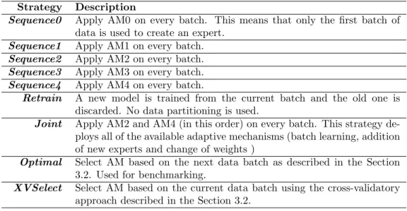
Strategy Description

Sequence0 Apply AM0 on every batch. This means that only the first batch of data is used to create an expert.

Sequence1 Apply AM1 on every batch.

Sequence2 Apply AM2 on every batch.

Sequence3 Apply AM3 on every batch.

Sequence4 Apply AM4 on every batch.

Retrain A new model is trained from the current batch and the old one is discarded. No data partitioning is used.

Joint Apply AM2 and AM4 (in this order) on every batch. This strategy de-ploys all of the available adaptive mechanisms (batch learning, addition of new experts and change of weights )

Optimal Select AM based on the next data batch as described in the Section 3.2. Used for benchmarking.

XVSelect Select AM based on the current data batch using the cross-validatory approach described in the Section 3.2.

Table 2: Adaptive strategies

5.2. Catalyst Activation Dataset

This data set was used for the NiSIS 2006 competition [37]. It includes 14 sensor measurements like flows, concentrations and temperatures from a real process. The target variable is the simulation of catalyst’s activity inside the reactor. The description of the reaction speed is taken from the literature, showing a strong non-linear dependency on temperature. Further complicated processes like cooling and catalyst decay contribute to changes in the data. The data set covers one year of operation of the plant. Many of the features exhibit high co-linearity and contain high number of outliers. The data includes 5,867 data samples. We have removed two features with mostly missing and 0 values during the preprocessing. The number of latent vectors for PLS was experimentally set to 12.

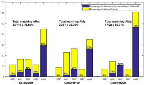
In the Table 3 we present the results with batch sizes of 50, 100 and 200, (Catalyst50, Catalyst100 and Catalyst200). The best result in terms of MAE among the methods with flexible AM deployment order are denoted with a†, and among the methods with fixed order with‡. We check whether the error values of these two strategies are significantly different with a significance level,α= 5%, and if so mark the most accurate strategy with a bold font. RC at the end of the strategy name denotes that the retrospective model correction was used. Using the benchmark (Optimal) strategy AM, which minimizes MAE for the incoming batch of data, always led to the lowest MAE for the whole dataset. On the smallest batch size of 50, the best method among methods with flexible AM sequences is XVSelect with correction and among the methods with fixed one is Sequence2. On the larger batch sizes respectivelyXVSelect, Retrain and Joint perform better in the respective groups. This can be a sign of the growing independence of the current data from historical data for this particular dataset, which is indeed known to be comparatively volatile. The distribution of the AMs inOptimal strategy and to what extentXVSelect AMs match with them is shown in the Figure 4. It is noticeable that

Batch size 50 100 200

Strategy MAE MSE MAE MSE MAE MSE

Fixed Order Sequence0 0.310 0.342 0.279 0.313 0.361 0.397 Sequence1 0.138 0.260 0.147 0.260 0.161 0.288 Sequence2 0.023‡ 0.067 0.031 0.067 0.058 0.139 Sequence4 0.037 0.062 0.031 0.062 0.052 0.095 Joint 0.035 0.074 0.035 0.074 0.049‡ 0.085 Retrain 0.024 0.081 0.028‡ 0.058 0.052 0.108 Flexible Order Sequence0 RC 0.031 0.081 0.045 0.081 0.072 0.109 Sequence1 RC 0.026 0.081 0.042 0.081 0.073 0.125 Sequence2 RC 0.026 0.081 0.039 0.081 0.073 0.123 Sequence3 RC 0.026 0.082 0.046 0.082 0.067 0.094 Sequence4 RC 0.021 0.075 0.034 0.075 0.053 0.097 Joint RC 0.020 0.082 0.035 0.082 0.052 0.095 XVSelect 0.020 0.055 0.029† 0.055 0.049† 0.096 XVSelect RC 0.018† 0.075 0.032 0.075 0.051 0.097 Optimal 0.015 0.031 0.024 0.049 0.040 0.069 Table 3: Catalyst dataset results

AM4 is the most common AM in theOptimal strategy, meaning that it often delivers the most accurate results. This is also the reason why it is often selected byXVSelect. On Catalyst100 dataset,XVSelect andOptimal have the least common AMs (Figure 4). This is also reflected in the Table 3, where for that caseRetrain has the least MAE.

AM0 AM1 AM2 AM3 AM4 AM0 AM1 AM2 AM3 AM4 AM0 AM1 AM2 AM3 AM4

0 10 20 30 40 50 60 70 15% 26% 42% 31% 65% 0% 8% 27% 0% 75% 0% 25% 100% 0% 76% Percentage of AMs correctly identified by XVSelect RC Percentage of AMs in Optimal

Catalyst100 Catalyst200

Catalyst50 Total matching AMs: 53/116 = 45.69%

Total matching AMs: 20/57 = 35.09%

Total matching AMs: 17/28 = 60.71%

Figure 4: AMs in Optimal strategy for the Catalyst dataset

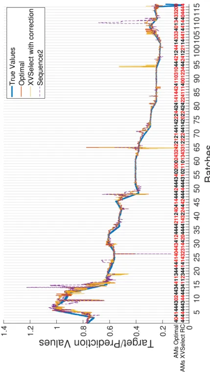
Figure 5 compares the true target values and predicted values of XVSelect with correction and Sequence2 on Catalyst50 dataset. The AMs deployed by Optimal and

XVSelect are also shown, marked red when they differ. We can see that in the beginning of the dataset, where the target value changes quite fast, algorithms with flexible AMs perform noticeably better. In the more stable parts of the data, such as batches 50-65 or 85-94, the differences are much less drastic. Optimal and XVSelect with correction can suffer from fluctuations (e.g. batches 107-108) which is an artefact of the SABLE algorithm, depending on its settings.

The importance of the proper selection of AMs is illustrated in Figure 6 which presents MAE values after exhaustively deploying all possible combinations of AMs for four steps ahead at every batch on the Catalyst50 dataset. As we can see in this figure, the choice of the wrong AM can result in a drastic increase in the prediction error.

We have additionally experimented with 2 and 3 steps retrospective correction as described in the Equation 7 for XVSelect. Figure 7 (a) shows the results. It can be seen that using more than one step retrospective correction does not generally bring improvement to the predictive accuracy, and in fact often decreases it. We relate this to the fact that using more retrospective correction steps increases the overfitting of the model to the current batch.

5.3. Thermal Oxidizer Dataset

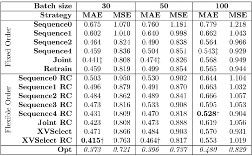
This dataset deals with the prediction of the concentration of exhaust gas during an industrial process where the task is to predict the concentrations ofN Oxin the exhaust gases. The data set consists of 36 input features which are hard sensor measurements. They are physical values like concentrations, flows, pressures and temperatures measured during the operation of the plant. The dataset consists of 2,820 samples. In addition, outliers and missing values are present in the data. The number of latent vectors for PLS was experimentally set to 3. In Table 4 we present the results with batch sizes of 30, 50 and 100 (Oxidizer30, Oxidizer50 and Oxidizer100).

Batch size 30 50 100

Strategy MAE MSE MAE MSE MAE MSE

Fixed Order Sequence0 0.675 1.070 0.760 1.181 0.779 1.218 Sequence1 0.602 1.010 0.640 0.998 0.662 1.043 Sequence2 0.464 0.824 0.490 0.838 0.564 0.966 Sequence4 0.459 0.836 0.504 0.851 0.543‡ 0.929 Joint 0.441‡ 0.808 0.474‡ 0.826 0.568 0.949 Retrain 0.459 0.819 0.499 0.854 0.565 0.944 Flexible Order Sequence0 RC 0.503 0.950 0.530 0.902 0.644 1.104 Sequence1 RC 0.496 0.879 0.491 0.870 0.663 1.032 Sequence2 RC 0.484 0.862 0.489 0.841 0.666 1.057 Sequence3 RC 0.473 0.816 0.533 0.908 0.595 1.053 Sequence4 RC 0.431 0.809 0.470 0.818 0.528† 0.904 Joint RC 0.423 0.808 0.473 0.888 0.619 1.056 XVSelect 0.471 0.866 0.484 0.903 0.570 0.931 XVSelect RC 0.415† 0.763 0.464† 0.817 0.553 1.019 Opt 0.373 0.721 0.396 0.737 0.480 0.829 Table 4: Oxidizer dataset results

Batches

Target/Prediction Values

True Values Optimal XVSelect with correction Sequence2

AMs XVSelect RC

AMs Optimal

Batches

MAE

Figure 6: 4 step ahead exhaustive deployment of all AMs on Catalyst50 dataset (gray). Red line shows

MAE values ofOptimalstrategy.

RC steps 0 1 2 3 Batch size 0 50 60 70 80 90 100 110 120 130 140 150 160 170 180 190 200 (a) -1 -0.5 0 0.5 1 RC steps 0 1 2 3 Batch size 0 30 40 50 60 70 80 90 100 (b) -1 -0.5 0 0.5 1 RC steps 0 1 2 3 Batch size 0 50 60 70 80 90 100 110 120 130 140 150 160 170 180 190 200 (c) -1.5 -1 -0.5 0 0.5 1 1.5

Figure 7: NormalizedXVSelectresults’ comparison with different batch sizes. White is the minimal and

black is the maximal error. (a) Catalyst dataset (b) Oxidizer dataset (c) Drier dataset.

The best results in this dataset are achieved with SABLE strategies with flexible AM deployment order -XVSelect with correction andSequence4 with correction. The most accurate strategies with fixed order areJoint and Sequence4. We see that for the

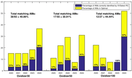
Oxidizer dataset, the strategies which rely more on historical data provide better results, as compared to the Catalyst dataset. This would seem to indicate the relatively lower volatility of the current dataset. Here, as shown in the Figure 8, AM4 is most often the best AM. It is however less dominant than in the Catalyst dataset. For this dataset, the probability of AMs being the best one is more evenly distributed than for the Catalyst data. This may be the the reason for less common AMs betweenOptimal andXVSelect than in the Catalyst dataset. Among three batch size settings, this percentage is the lowest on the Oxidizer50. This is reflected in comparatively low predictive accuracy of theXVSelect for that case.

AM0 AM1 AM2 AM3 AM4 AM0 AM1 AM2 AM3 AM4 AM0 AM1 AM2 AM3 AM4

0 10 20 30 40 50 60 21% 21% 29% 53% 56% 17% 25% 31% 25% 41% 17% 33% 0% 100% 57%

Percentage of AMs correctly identified by XVSelect RC Percentage of AMs in Optimal

Oxidizer50 Oxidizer100 Oxidizer30

Total matching AMs: 38/93 = 40.86%

Total matching AMs: 17/55 = 30.91%

Total matching AMs: 12/27 = 44.44%

Figure 8: AMs in Optimal strategy for the Oxidizer dataset

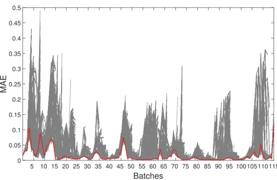
Figure 9 compares the true target values and predicted values of XVSelect with correction andJoint on Oxidizer30 dataset. The AMs deployed by Optimal and XVSelect are also shown and marked red when they differ. We can see that the Oxidizer dataset has a cyclic characteristic, with extreme values roughly every 5 batches. Often after these extreme values,Joint prediction values show higher errors (e.g. batches #8, #13, #17, #30, etc.). We relate this to the strong adaptation of this strategy, which overfits the model to the extreme valuesXVSelect in contrast behaves more stable with less obvious jumps (e.g. batches #57, #76, #80) to extreme values. As seen in Figure 10 the order of AMs makes a large difference for predicting on the Oxidizer dataset as well. As seen in Figure 10 the order of AM can make a large difference in the prediction accuracy for the Oxidizer dataset. Figure 7 (b) shows that also for this dataset using more than one step retrospective correction in most cases does not improve the predictive accuracy, and often causes its deterioration.

5.4. Industrial Drier Dataset

The target value of this dataset describes the laboratory measurements of the residual humidity of the process product. The dataset has 19 input features, most of them being

Batches

Target/Prediction Values

True Values Optimal XVSelect with correction Joint

AMs Optimal

AMs XVSelect RC

Batches

MAE

Figure 10: 4 step ahead exhaustive deployment of all AMs on Oxidizer30 dataset (gray). Red line shows

MAE values ofOptimalstrategy.

temperatures, pressures and humidities measured in the processing plant. The original dataset consists of 1,219 data samples covering almost seven months of the operation of the process. It consists of raw unprocessed data as recorded by the process information and measurement system. Many of the input variables show problems common in indus-trial data like measurement noise, missing values or data outliers. We have removed 3 input features which mostly consisted of missing data. The number of latent variables for PLS was experimentally set to 16. In Table 5 we present the results with batch sizes of 50, 100 and 200, denoted respectively Drier50, Drier100 and Drier200.

From the results, it is obvious that the Drier dataset is the most stable out of the ones we have experimented with. The plot of the Drier50 dataset target values is shown in Figure 1111_{. For lower batch sizes, simple RPLS on-line updateSequence1 performs} as good, or better than strategies with stronger adaptation or flexible AM deployment order. For the largest batch size of 200 however, XVSelect shows the most accurate predictions. In fact in this case it deploys exactly the same AMs as Optimal. It is worth noting that for this dataset there are only 5 batches of the test data for the batch size of 200. As seen from the Figure 12, AM0 is prevalent AM for this dataset. We relate this to the lack of changes in the data. This is why the number of times when XVSelect andOptimal deploy the same AMs is greater than in the two other datasets. The Figure 10 also confirms that the order of AMs makes less difference on the predictive

11_{We do not show predictions for this dataset, as their errors are much smaller than the axis scale,}

making them impossible to distinguish from the target values. 20

Batch size 50 100 200

Strategy MAE MSE MAE MSE MAE MSE

Fixed

Order

Sequence0 7.68E-04 8.67E-04 5.41E-04 5.97E-04 3.87E-04 4.07E-04

Sequence1 8.98E-06‡ 2.57E-05 8.09E-06‡ 2.04E-05 5.06E-05 1.43E-04

Sequence2 3.04E-05 2.04E-04 1.75E-05 1.15E-04 5.28E-05 1.44E-04

Sequence4 9.86E-05 3.41E-04 1.43E-05 8.30E-05 8.77E-05 1.92E-04

Joint 4.06E-05 2.40E-04 1.34E-05 8.28E-05 5.01E-05‡ 1.43E-04

Retrain 5.86E-05 3.14E-04 2.59E-05 1.54E-04 5.38E-05 1.44E-04

Flexible

Order

Sequence0 RC 9.78E-06 7.02E-05 1.43E-05 5.39E-05 1.34E-04 2.42E-04

Sequence1 RC 1.02E-05 4.56E-05 8.96E-06† 2.09E-05 5.41E-05 1.43E-04

Sequence2 RC 3.02E-05 1.41E-04 1.79E-05 1.15E-04 5.09E-05 1.43E-04

Sequence3 RC 9.78E-06 7.02E-05 1.44E-05 5.39E-05 1.34E-04 2.42E-04

Sequence4 RC 4.06E-05 2.40E-04 1.34E-05 8.28E-05 6.41E-05 1.64E-04

Joint RC 4.16E-05 2.40E-04 1.37E-05 8.28E-05 5.01E-05 1.43E-04

XVSelect 9.27E-06 4.02E-05 1.20E-05 3.08E-05 4.67E-05† 1.43E-04

XVSelect RC 6.95E-06† 3.99E-05 1.12E-05 3.06E-05 4.67E-05† 1.43E-04

Optimal 3.40E-06 3.47E-05 3.15E-06 1.15E-05 4.67E-05 1.43E-04 Table 5: Drier dataset results

accuracy for this dataset, except around the batches #6-#7. Figure 7 (c) shows that as opposed to the previous datasets, predictive accuracy on Drier data usually improves when increasing retrospective correction steps. This can be also related to the stability of the dataset, where stronger optimization of the model towards the current batch does not cause overfitting issues.

Batches 5 10 15 20 Target Values -10 -8 -6 -4 -2 0 2 4 6 8 10

Figure 11: Drier50 dataset target values

AM0 AM1 AM2 AM3 AM4 AM0 AM1 AM2 AM3 AM4 AM0 AM1 AM2 AM3 AM4 0 10 20 30 40 50 60 70 80 82% 67% 67% 100% 50% 0% 100% 0% 100% 100%

Percentage of AMs correctly identified by XVSelect RC Percentage of AMs in Optimal

Drier200 Drier100

Drier50 Total matching AMs: 18/23 = 78.26%

Total matching AMs: 5/11 = 45.45%

Total matching AMs: 5/5 = 100%

Figure 12: AMs in Optimal strategy for the Drier dataset

Batches

MAE

Figure 13: 4 step ahead exhaustive deployment of all AMs on Drier50 dataset (gray). Red line shows

MAE values ofOptimalstrategy.

6. Discussion and Conclusions

The core aim of this paper was to investigate the behaviour of a data-driven soft sensor with multiple adaptive mechanisms. We have conducted experiments on 3 real₂₂

datasets from the process industry, exhibiting different properties and different rates of change.

We observe that in most of the cases, using multiple AMs is better than using only one, even the most suitable AM for the dataset. This is true for Catalyst and Oxidizer datasets. Here, having the possibility to deploy AMs which are rarely the best, brings an improvement to the predictive accuracy of the soft sensor. For the Drier dataset, using just AM1 (batch learning with no forgetting) provides good results. This is related to the lack of change in dataset - hence the AMs which apply stronger adaptation to the models are not needed and overcomplicate the model.

Similarly, using SABLE with flexible AM deployment strategies provided better re-sults for most of the cases. Here the comparison is mostly betweenJoint (deploying all of the available AMs on the same batch) and flexible configurations. We have seen that choosing the AM which minimizes the error for the next batch (Optimal configuration) provides better results thanJoint.

As shown in [10],XVSelect(using cross-validatory selection based on the last available batch) achieves quite high predictive accuracy levels. This can be further improved by retrospective AM correction mechanism. Generally XVSelect strategy with correction provides the best predictive accuracy in most of the cases.

Considering all of the above, we can conclude that in a batch learning scenario, using multiple adaptive mechanisms with flexible deployment order which is identified using cross-validatory selection together with the application of retrospective model correction provides significantly better results than simple retraining, deployment of separate AMs and their joint deployment on every batch.

7. Acknowledgements

Research leading to these results has received funding from the EC within the Marie Curie Industry and Academia Partnerships and Pathways (IAPP) programme under grant agreement no. 251617. The authors would like to thank Evonik Industries AG for the provided datasets and J. Czeczot for the insightful discussion. Part of the used Matlab code originates from P. Kadlec and R. Grbi´c [8].

Appendix A. Notation

Symbol Meaning F orm ulation y Actual output ˆ y Predicted output x Input instance τ Time k Batch number

Vk Data batch at timek,Vk={Xk,yk} nk Size ofk-th batch

ψ Function of the real process which generates the data f Prediction function/expert (indexed 1· · ·I)

f− A priori prediction function (before the adaptation) f+ _{A posteriori prediction function (after the adaptation)}

g Adaptive Mechanism (AM) (indexed 1· · ·H) ghk AM chosen at batchk

G Set of available AMs

S Cross-validation training subset

S Cross-validation test subset

h i Error measure

h i× _{Cross-validated error measure}

Noise

Θf Set of parameters off Θg Set of parameters ofg

r Retrospective Correction step

SABLE

m Feature number

Di,m Descriptor ofm-th feature ofi-th expert

D Descriptors matrix Vtr _{Training data}

w(xj) Weight forj-th instance Φ(µm

j ,Σ) Two-dimensional Gaussian kernel function µ= (xm_j , yj) Mean value of Gaussian kernel function

Σ Variance matrix of kernel function withσ at the diagonal positions σ Kernel width

vi Weight ofi-th expert’s prediction p(˙) Probability

F Set of experts

RPLS

N Number of data instances M Number of input variables

C Number of output variables L Number of latent variables

T Score matrix

t Latent vector

S Corresponding loading matrix

s Column vector ofS U Score matrix

u Latent vector

Q Corresponding loading matrix

q Column vector ofQ E Input data residual

F Output data residual

B Regression weights matrix

b Column vector ofB

ˆ

Y Estimates ofY

λ Forgetting factor

Results α Significance level

Table A.6: Notation 24

References

[1] P. Kadlec, B. Gabrys, S. Strandt, Data-driven Soft Sensors in the process industry, Computers & Chemical Engineering 33 (2009) 795–814.

[2] A. Cinar, S. J. Parulekar, C. Undey, G. Birol, Batch Fermentation: Modeling: Monitoring, and Control, CRC Press, 2003.

[3] G. G. B. Neal B. Gallagher, Barry M. Wise, Stephanie Watts Butler, Daniel D. White, Jr., Devel-opment And Benchmarking Of Multivariate Statistical Process Control Tools For A Semiconductor Etch Process: Improving Robustness Through Model Updating, in: Process: Impact of Measure-ment Selection and Data TreatMeasure-ment on Sensitivity, Safeprocess 97, pp. 26–27.

[4] J. C. Schlimmer, R. H. Granger, Beyond incremental processing: Tracking Concept Drift, AAAI-86 Proceedings (1986) 502–507.

[5] P. Kadlec, R. Grbi´c, B. Gabrys, Review of adaptation mechanisms for data-driven soft sensors,

Computers & Chemical Engineering 35 (2011) 1–24.

[6] B. S. Dayal, J. F. MacGregor, Recursive exponentially weighted PLS and its applications to adaptive control and prediction, Journal of Process Control 7 (1997) 169–179.

[7] W. Li, H. Yue, S. Valle-Cervantes, S. Qin, Recursive PCA for adaptive process monitoring, Journal of Process Control 10 (2000) 471–486.

[8] P. Kadlec, B. Gabrys, Local learning-based adaptive soft sensor for catalyst activation prediction, AIChE Journal 57 (2011) 1288–1301.

[9] H. Jin, X. Chen, J. Yang, H. Zhang, L. Wang, L. Wu, Multi-model adaptive soft sensor modeling method using local learning and online support vector regression for nonlinear time-variant batch processes, Chemical Engineering Science 131 (2015) 282–303.

[10] R. Bakirov, B. Gabrys, D. Fay, On sequences of different adaptive mechanisms in non-stationary regression problems, in: 2015 International Joint Conference on Neural Networks (IJCNN), pp. 1–8. [11] S. Joe Qin, Recursive PLS algorithms for adaptive data modeling, Computers & Chemical

Engi-neering 22 (1998) 503–514.

[12] R. Grbi´c, D. Sliˇskovi´c, P. Kadlec, Adaptive soft sensor for online prediction and process monitoring

based on a mixture of Gaussian process models, Computers & Chemical Engineering 58 (2013) 84–97.

[13] H. Kaneko, K. Funatsu, Adaptive soft sensor based on online support vector regression and Bayesian ensemble learning for various states in chemical plants, Chemometrics and Intelligent Laboratory Systems 137 (2014) 57–66.

[14] H. Kaneko, K. Funatsu, Ensemble locally weighted partial least squares as a just-in-time modeling method, AIChE Journal (2015).

[15] S. Gomes Soares, R. Ara´ujo, An on-line weighted ensemble of regressor models to handle concept

drifts, Engineering Applications of Artificial Intelligence 37 (2015) 392–406.

[16] S. Gomes Soares, R. Ara´ujo, A dynamic and on-line ensemble regression for changing environments,

Expert Systems with Applications 42 (2015) 2935–2948.

[17] F. Souza, R. Ara´ujo, Online Mixture of Univariate Linear Regression Models for Adaptive Soft

Sensors, in: IEEE Transactions on Industrial Informatics, volume 10, pp. 937–945.

[18] H. Jin, X. Chen, J. Yang, L. Wu, Adaptive soft sensor modeling framework based on just-in-time learning and kernel partial least squares regression for nonlinear multiphase batch processes, Computers & Chemical Engineering 71 (2014) 77–93.

[19] W. Shao, X. Tian, P. Wang, Local Partial Least Squares Based Online Soft Sensing Method for Multi-output Processes with Adaptive Process States Division, Chinese Journal of Chemical Engi-neering 22 (2014) 828–836.

[20] W. Ni, S. D. Brown, R. Man, A localized adaptive soft sensor for dynamic system modeling, Chemical Engineering Science 111 (2014) 350–363.

[21] H. Jin, X. Chen, J. Yang, L. Wang, L. Wu, Online local learning based adaptive soft sensor and its application to an industrial fed-batch chlortetracycline fermentation process, Chemometrics and Intelligent Laboratory Systems 143 (2015) 58–78.

[22] W. Shao, X. Tian, Adaptive soft sensor for quality prediction of chemical processes based on selective ensemble of local partial least squares models, Chemical Engineering Research and Design 95 (2015) 113–132.

[23] W. Shao, X. Tian, P. Wang, X. Deng, S. Chen, Online soft sensor design using local partial least squares models with adaptive process state partition, Chemometrics and Intelligent Laboratory Systems 144 (2015) 108–121.

[24] W. Shao, X. Tian, P. Wang, Soft sensor development for nonlinear and time-varying processes 25

based on supervised ensemble learning with improved process state partition, Asia-Pacific Journal of Chemical Engineering 10 (2015) 282–296.

[25] J. Bates, C. Granger, The combination of forecasts, OR 20 (1969) 451–468.

[26] R. A. Jacobs, M. I. Jordan, S. J. Nowlan, G. E. Hinton, Adaptive mixtures of local experts, Neural Comput. 3 (1991) 79–87.

[27] P. Kadlec, B. Gabrys, Soft sensor based on adaptive local learning, Advances in Neuro-Information Processing (2009).

[28] P. Kadlec, B. Gabrys, Adaptive on-line prediction soft sensing without historical data, in: The 2010 International Joint Conference on Neural Networks (IJCNN), IEEE, 2010, pp. 1–8.

[29] H. Wold, Estimation of Principal Components and Related Models by Iterative Least squares, Academic Press, New York, 1966, pp. 391–420.

[30] H. Drucker, C. Burges, L. Kaufman, A. Smola, V. Vapnik, Support Vector Regression Machines, Neural Information Processing Systems 1 (1996) 155–161.

[31] H. Kaneko, T. Okada, K. Funatsu, Selective Use of Adaptive Soft Sensors Based on Process State, Industrial & Engineering Chemistry Research 53 (2014) 15962–15968.

[32] P. Kadlec, B. Gabrys, Architecture for development of adaptive on-line prediction models, Memetic Computing 1 (2009) 241–269.

[33] R. Bakirov, B. Gabrys, D. Fay, Augmenting Adaptation with Retrospective Model Correction for Non-Stationary Regression Problems, in: 2016 International Joint Conference on Neural Networks (IJCNN) - in print.

[34] E. Parzen, On Estimation of a Probability Density Function and Mode, The Annals of Mathematical Statistics 33 (1962) pp. 1065–1076.

[35] P. Geladi, B. R. Kowalski, Partial least-squares regression: a tutorial, Analytica Chimica Acta 185 (1986) 1–17.

[36] B. Mizrach, Forecast comparison in L2, Technical Report 908, Working Papers, No. 1995-24, Department of Economics, Rutgers, The State University of New Jersey, 1996. URL: http://www.econstor.eu/handle/10419/94277.

[37] J. Strackeljan, NiSIS Competition 2006 - Soft Sensor for the adaptive Catalyst

Moni-toring of a MultiTube Reactor, Technical Report, Universit¨at Magdeburg, 2006. URL:

http://www-staff.informatik.uni-frankfurt.de/asa/software/MI2/papers/Competition Summary for NiSIS 2006 booklet.pdf.

List of Figures

1 Adaptation with multiple AMs. Optional inputs are shown with dashed

lines. . . 5

2 Block diagram of SABLE model. . . 7

3 An example of a model adaptation sequence using SABLE AMs . . . 10

4 AMs in Optimal strategy for the Catalyst dataset . . . 14

5 Predictions on Catalyst50 dataset . . . 16

6 4 step ahead exhaustive deployment of all AMs on Catalyst50 dataset (gray). Red line shows MAE values of Optimal strategy. . . 17

7 NormalizedXVSelectresults’ comparison with different batch sizes. White is the minimal and black is the maximal error. (a) Catalyst dataset (b) Oxidizer dataset (c) Drier dataset. . . 17

8 AMs in Optimal strategy for the Oxidizer dataset . . . 18

9 Predictions on Oxidizer30 dataset . . . 19

10 4 step ahead exhaustive deployment of all AMs on Oxidizer30 dataset (gray). Red line shows MAE values of Optimal strategy. . . 20

11 Drier50 dataset target values . . . 21

12 AMs in Optimal strategy for the Drier dataset . . . 22

13 4 step ahead exhaustive deployment of all AMs on Drier50 dataset (gray). Red line shows MAE values ofOptimal strategy. . . 22