Outlier robust small area estimation

Wo

Meth

Ou

Est

Iray Ch

Abstrac

[Recently drawn fr leads to idea and corrected the prop squared

orkin

hodolog

utlier

tima

hambers,H

ct

y proposed rom a distrib the idea of d also propo d outlier rob posed bias co error estima

ng Pa

gy

r Rob

ation

Hukum Cha

outlier robu ution that ha an outlier ro ose two diff bust estimato orrection oft ators appear

aper

bust

n

andra,Nico

st small area as a different obust bias co ferent analyt ors. Simulati ten leads to to perform w

r M11

Sma

ola Salvati,N

a estimators t mean from orrection for tical mean s ons based o more efficie well with a va

1/07

all A

Nikos Tzav

s can be sub that of the r these estim squared erro on realistic o nt estimator ariety of outli

7

Area

vidis

bstantially bi est of the su ators. In this or estimator outlier contam s. Furthermo er robust sm iased when urvey data. Th s paper we d rs for the e minated data ore, the prop mall area esti

outliers are his naturally develop this nsuing bias a show that posed mean mators.]

Outlier Robust Small Area Estimation

Ray Chambers1

University of Wollongong, Australia Hukum Chandra

University of Wollongong, Australia Nicola Salvati

University of Pisa, Italy and Nikos Tzavidis

University of Southampton, United Kingdom.

Summary. Recently proposed outlier robust small area estimators can be substantially biased when outliers are drawn from a distribution that has a different mean from that of the rest of the survey data. This naturally leads to the idea of an outlier robust bias correction for these estimators. In this paper we develop this idea and also propose two different analytical mean squared error estimators for the ensuing bias corrected outlier robust estimators. Simulations based on realistic outlier contaminated data show that the proposed bias correction often leads to more efficient estimators. Furthermore, the proposed mean squared error estimators appear to perform well with a variety of outlier robust small area estimators.

Keywords: Bias-variance trade-off; Linear mixed model; M-estimation; M-quantile model; Robust prediction; Robust bias correction.

1. Introduction

Outliers are a fact of life for any survey and as a result, a variety of methods have been devised to mitigate the effects of outlier values on survey estimates. Some of these methods, like identification and removal of these data values by ‘experienced’ data experts during survey processing, can be effective in ensuring that the resulting survey estimates are unaffected by outliers. However, being somewhat subjective, such methods are not amenable to scientific evaluation. As a consequence there are a number of ‘objective’ methods for survey estimation that use statistical rules to decide whether an observation is a potential outlier and to down-weight its contribution to the survey estimates if this is the case. Generally, an outlier robust estimator of this type is based on the assumption that the non-outlier sample values all follow a well-behaved working model and so it generally involves prediction of the sum (or mean) of these values under this working model. In practice,

1 1_{Address for correspondence}

:Ray Chambers, Centre for Statistical and Survey Methodology, School of Mathematics and Applied Statistics, University of Wollongong, Wollongong, Australia. Email:[email protected]

this often involves replacement of an outlying sample value by an estimate of what it should have been if in fact it had been generated under the working model. We refer to such methods as Robust Projective in what follows since they project sample non-outlier behaviour on to the non-sampled part of the survey population.

Robust Projective methods essentially emulate the subjective approach described earlier, and typically lead to biased estimators with lower variances than would otherwise be the case. The reason for the bias is not difficult to find – it is extremely unlikely that the non-sampled values in the target population are drawn from a distribution with the same mean as the sample non-outliers, and yet these methods are built on precisely this assumption. Chambers (1986) recognised this dilemma and coined the concept of a ‘representative outlier’, i.e. a sample outlier that is potentially drawn from a group of population outliers and hence cannot be unit-weighted in estimation. He noted that representative outliers cannot be treated on the same basis in estimation as other sample data more consistent with the working model for the population, since such values can seriously destabilise the survey estimates, and suggested addition of an outlier robust bias correction term to a Robust Projective survey estimator, e.g. one based on outlier-robust estimates of the model parameters. Welsh and Ronchetti (1998) expand on this idea, applying it more generally to estimation of the finite population distribution of a survey variable in the presence of representative outliers. A similar idea is implicit in the approach described in Chambers et al. (1993), where a nonparametric bias correction is suggested. In what follows, we refer to methods that allow for contributions from representative sample outliers as Robust Predictive since they attempt to predict the contribution of the population outliers to the population quantity of interest.

If outliers are a concern for estimation of population quantities, it is safe to say that they are even more of a concern in small area estimation (SAE), where sample sizes are considerably smaller and model-dependent estimation is the norm. It is easy to see that an outlier that destabilises a population estimate based on a large survey sample will almost certainly destroy the validity of the corresponding direct estimate for the small area from which the outlier is sourced since this estimate will be based on a much smaller sample. This problem does not disappear when the small area estimator is an indirect one, e.g. an Empirical Best Linear Unbiased Predictor (EBLUP), since the weights underpinning this estimator will still put most

emphasis on data from the small area of interest, and the estimates of the model parameters underpinning the estimator will themselves be destabilised by the sample outliers. Consequently, it is of some interest to see how outlier robust survey estimation can be adapted to this situation.

Chambers and Tzavidis (2006) explicitly address this issue of outlier robustness, using an approach based on fitting outlier robust M-quantile models to the survey data. Recently, Sinha and Rao (2009) have also addressed this issue from the perspective of linear mixed models. Both these approaches, however, use plug-in robust prediction. That is, they replace parameter estimates in optimal, but outlier sensitive, predictors by outlier robust versions (a Robust Projective approach). Unfortunately, this approach may involve an unacceptable prediction bias (but a low prediction variance) in situations where the outliers are drawn from a distribution that has a different mean to the rest of the survey data.

After discussing Robust Projective estimators for small areas in Section 2, we explore the extension of Chambers (1986) Robust Predictive approach to the SAE situation in Section 3. In Section 4 we propose two different analytical mean squared error (MSE) estimators for outlier robust predictors of small area means. In particular, the first proposal is based on the bias-robust mean squared error estimation approach described in Chambers et al. (2009) and represents an extension of the ideas in Royall and Cumberland (1978). The second MSE estimator is based on first order approximations to the variances of solutions of estimating equations. We show how these two approaches can be useful for estimating the MSE of various small area predictors considered in this paper. In Sections 5 and 6 we use model-based simulations based on realistic outlier contaminated data scenarios as well as design-based simulations to evaluate how these two different approaches compare, both in terms of point estimation performance as well as in terms of MSE estimation performance. Section 7 concludes the paper with some final remarks, and a discussion of future research aimed at outlier robust small area inference.

2. Robust Projective Estimation for Small Areas

In what follows we assume that unit record data are available at small area level. For the sampled units in the population this consists of indicators of small area affiliation, values y_j of the variable of interest, values

j

the non-sampled population units we do not know the values of y_j. However, it is assumed that all areas are sampled and that we know the numbers of such units in each small area and the respective small area averages of x_j and z_j. We also assume that there is a linear relationship between y_j and x_j and that sampling is non-informative for the small area distribution of yj given xj, allowing us to use population

level models with the sample data.

A popular way of using the above data in SAE is to assume a linear mixed model, with random effects for the small areas of interest (see Rao, 2003). Let y, X and Z denote the population level vector and

matrices defined by yj, xj and zj respectively. Then

= + +

y Xββββ Zu e, (1)

where =

(

₁T,…, T

)

T

m

u u u is a vector of dimension mq made up of m independent realisations

{ ; =1,…, }

i i m

u of a q-dimensional random area effect with ∼ ( , )

u N u 0ΣΣΣΣ and ∼ ( , ) e N e 0 ΣΣΣΣ is a vector of

N individual specific random effects. It is also assumed that

u

is distributed independently of

e

.Here m is the total number of small areas that make up the population and q is the dimension of zj so that Z is a

×

N mq matrix of fixed known constants. We assume that the covariance matrices ΣΣΣΣ_u and ΣΣΣΣ_e are defined in terms of a lower dimensional set of parameters =( ,θ₁…,θ )

K

θ θθ

θ , which are typically referred to as the variance components of (1), while ββββ is usually referred to as its fixed effect.

Let ˆββββ and ˆu denote estimates of the fixed and random effects in (1). The EBLUP of the area i

mean of the y_j under (1) is then

(

)

(

)

{

}

1 _ˆ ˆ − _ˆ = + − + EBLUP T T i i i si i i ri ri y N n y N n x ββββ z u , (2) where ˆ =

(

ˆ₁T,…, ˆT

)

T m

u u u denotes the vector of the estimated area specific random effects and we use

indices of s and r to denote sample and non-sample quantities respectively. Thus, y_si is the average of the

i

n sample values of y_j from area i and x_ri and z_ri denoting the vectors of average values of x_j and

j

z respectively for the N_i−n_i non-sampled units in the same area.

From a Robust Projective viewpoint, (2) can be made insensitive to sample outliers by replacing ˆββββ

and ˆu by outlier robust alternatives. To motivate this approach, we initially assume the variance

= + T s es s u s

V ΣΣΣΣ Z ΣΣΣΣ Z where ΣΣΣΣ_es denotes the sample component of ΣΣΣΣ_e. Then the BLUE of the fixed effects vector ββββ is

{

₋₁

}

−1 ₋₁ = T T s s s s s s X V X X V y β ββ β , (3)

while the BLUP of the random effects vector u is

(

)

1 − = Σ − T u s s s s u Z V y X ββββ . (4)

It is easy to see that (3) and (4) are solutions to

(

)

1 − − = T s s s s X V y X ββββ 0 (5) and

(

)

1 − − − = T uZ Vs s ys Xsββββ u 0 Σ ΣΣ Σ . (6)

A straightforward way to make the solutions to (5) and (6) robust to sample outliers is therefore to replace them by

{

}

(

)

1/ 2_ψ 1/ 2 − − − = T s s s s s X V V y X ββββ 0 (7) and

{

}

(

)

(

)

1/ 2_ψ 1/ 2 _β 1/ 2_ψ 1/ 2 − − − − − = T uZ Vs s Vs ys Xs u u u 0 Σ Σ Σ Σ Σ Σ Σ Σ Σ Σ Σ Σ . (8)

Here ψ is a bounded influence function and ψ( )a denotes the vector defined by applying ψ to every component of a. Unfortunately, since V_s is not a diagonal matrix, the solution to (8) can be numerically unstable. An alternative approach was therefore suggested by Fellner (1986), who noted that any solution to (5) and (6) was also a solution to

(

)

1 − − − = T s es s s s X ΣΣΣΣ y X ββββ Z u 0 and −1

(

)

−1 − − − = T s es s s s u Z ΣΣΣΣ y X ββββ Z u ΣΣΣΣ u 0.

Fellner (1986) suggested that these alternative estimating equations (and hence their solutions) be made outlier robust by replacing them by

{

}

(

)

1/ 2_ψ 1/ 2 − − − − = T s es es s s s X ΣΣΣΣ ΣΣΣΣ y X ββββ Z u 0 (9) and

{

}

(

)

(

)

1/ 2_ψ 1/ 2 1/ 2_ψ 1/ 2 − − − − − − − = T s es es s s s u u Z ΣΣΣΣ ΣΣΣΣ y X ββββ Z u ΣΣΣΣ ΣΣΣΣ u 0. (10)

limited unless outlier robust estimators of these parameters can also be defined. Richardson and Welsh (1995) propose two outlier robust variations to the maximum likelihood estimating equations for θθθθ. One of these (ML Proposal II) leads to an estimating equation for the variance component θk of θθθθ of the form

(

)

{

1/ 2

}

1/ 2

(

)

1/ 2

{

1/ 2

(

)

}

{

ψ

(

)

}

ψ − − θ − ψ − θ − T ∂ ∂ − = ∂ ∂ s s s s s k s s s s tr n s k y X ββββ V V V V V y X ββββ D V , (11)

where ∂V_s ∂θ_k denotes the first order partial derivative of V_s with respect to the variance component θ_k

and, for _Z∼_N(0,1)_, ψ

{

_ψ2_{( )}

}

−1

=

n E Z s

D V .

Sinha and Rao (2009) describe an approach to outlier robust estimation of ββββ and u in (1) that builds on these results, substituting approximate solutions to both (7) and (11) into the Fellner estimating equation (10) to obtain an outlier robust estimate of the area effect u. In particular, their approach replaces

(7) by

{

}

(

)

1 1/ 2_ψ 1/ 2 − − − = T s s s s s s X V U U y X ββββ 0, (12)

where U_s =diag

( )

V_s , and replaces (11) by

(

)

{

1/ 2

}

1/ 2 1

(

)

1 1/ 2

{

1/ 2

(

)

}

{

(

)

}

. ψ ψ − − θ − ψ − θ − T ∂ ∂ − = ∂ ∂ s s s s s s k s s s s s tr n s k y X ββββ U U V V V U U y X ββββ D V (13)

Since the solutions to (12) and (13) depend on the influence function ψ , we denote them by a superscript of ψ below. The Sinha and Rao (2009) Robust Projective alternative to (2) is then

ˆ

ˆSR₌ T ψ ₊ T_ˆψ

i i i

y x ββββ z u . (14)

Note that (14) estimates the area i mean under (1). A minor modification restricts this to the mean of the non-sampled units in area i, in which case (14) becomes

(

)

(

)

{

}

1 _ˆ ˆ − ψ _ˆψ = + − + REBLUP T T i i i si i i ri ri y N n y N n x ββββ z u . (15)

Hereafter we call this estimator the Robust EBLUP (REBLUP). An alternative methodology for outlier robust SAE is the M-quantile regression-based method described by Chambers and Tzavidis (2006). This is based on a linear model for the M-quantile regression of y on X, i.e.

( )=

q q

m X Xββββ , (16)

where m_q( )X denotes the M-quantile of order q of the conditional distribution of y given X. An estimate ˆββββ_q of ββββ_q can be calculated for any value of q in the interval (0,1), and for each unit in sample

we define its unique M-quantile coefficient under this fitted model as the value q_j such that = ˆ

j

T j j q

y x ββββ , with the sample average of these coefficients in area i denoted by q_i. The M-quantile estimate of the mean of y_j in area i is then

(

)

{

}

1 _ˆ ˆ − = + − i MQ T i i i si i i ri q y N n y N n x ββββ . (17)

Note that the regression M-quantile model (16) depends on the influence function ψ underpinning the M-quantile. When this function is bounded, sample outliers have limited impact on ˆββββ_q. That is, (17) corresponds to assuming that all non-sample units in area i follow the working model (16) with q=q_i, in

the sense that one can write = + noise

i

T j j q

y x ββββ for all such units.

3. Robust Predictive Estimation for Small Areas

A problem with the Robust Projective approach is that it assumes all non-sampled units follow the working model, or, in what essentially amounts to the same thing, that any deviations from this model are noise and so cancel out ‘on average’. Thus, under the linear mixed model (1) one can see that provided the individual errors of the non-sampled units are symmetrically distributed about zero, the REBLUP (15) by Sinha and Rao (2009) will perform well since it is based on the implicit assumption that the average of these errors over the non-sampled units in area i converges to zero. The M-quantile estimator MQ (17) is no different since it assumes that the errors −

i

T j j q

y x ββββ from the area i-specific M-quantile regression model are ‘noise’ and hence also cancel out on average. Note that this does not mean that these non-sample units are not outliers. It is just that their behaviour is such that our best prediction of their corresponding average value is zero.

Welsh and Ronchetti (1998) consider the issue of outlier robust prediction within the context of population level survey estimation. Starting with a working linear model linking the population values of yj

and x_j, and sample data containing representative outliers with respect to this model, they extend the approach of Chambers (1986) to robust prediction of the empirical distribution function of the population values of y_j. Their argument immediately applies to robust prediction of the empirical distribution function of the area i values of yj, and leads to a predictor of the form

(

)

{

}

(

)

1 1 _{ˆ ˆ} ˆψφ_{( )} − _{( )} − ψ _{ω φ}ψ ψ _ωψ ∈ ∈ ∈   =  ≤ + + − ≤  

∑

i

∑∑

i i  T T i i j i k ij j j ij j s j s k r F t N I y t n I x ββββ y x ββββ t . (18)

Here ˆββββψ denotes an M-estimator of the regression parameter in the linear working model based on a

bounded influence function ψ , ωψ_ij is a robust estimator of the scale of the residual − T ˆψ j j

y x ββββ in area i

and φ denotes a bounded influence function that satisfies φ ≥ψ . Tzavidis et al. (2010) note that the robust estimator of the area i mean of the y_j defined by (18) is just the expected value functional defined by it, which is

(

)

{

(

)

}

1 _ˆ 1 _ˆ ˆ ˆψφ ψφ_{( )} − ψ − _{ω φ}ψ ψ _ωψ ∈    = =  + − _ + − _    

∑



∫

i T T i i i i si i i ri i ij j j ij j s y tdF t N n y N n x ββββ n y x ββββ . (19)

These authors therefore suggest an extension to the M-quantile estimator (17) by replacing ˆββββψ in (19) by

ˆ i q β β β

β , which leads to a ‘bias-corrected’ version of (17), hereafter MQ-BC, given by

(

)

{

(

)

}

1 _ˆ 1 _ˆ ˆ − − − _{ω φ ω} ∈    =  + − _ + − _     i

∑

i  i MQ BC T MQ T MQ i i i si i i ri q i ij j j q ij j s y N n y N n x ββββ n y x ββββ (20) and ωMQ

ij is a robust estimator of the scale of the residual − ˆ i

T j j q

y x ββββ in area i.

The use of the two influence functions ψ and φ in (20) is worthy of comment. The first, ψ , underpins ˆββββ_q, and hence ˆ

i

q

β ββ

β . Its purpose is to ensure that sample outliers have little or no influence on the fit of the working M-quantile model. As a consequence it is bounded and down-weights these outliers. The second, φ, is still bounded but ‘less restrictive’ than ψ (since φ ≥ψ ) and its purpose is to define an adjustment for the bias caused by the fact that the first two terms on the right hand side of (20) treat sample outliers as self-representing. A similar argument can be used to modify the REBLUP (15). In particular, a Robust Predictive version of this estimator, hereafter REBLUP-BC, mimics the bias correction idea used in (20) and leads to

(

1

)

1

{

(

_ˆ

)

}

ˆ − ˆ ₁ − − _{ω φ}ψ ψ _ˆψ _ωψ ∈ = + −

∑

− − i REBLUP BC REBLUP T T i i i i i ij j j j ij j s y y n N n y x ββββ z u , (21)

where the ωψ_ij are now robust estimates of the scale of the area i residuals − T ˆψ − Tˆψ

j j j

4. MSE Estimation for Robust Predictors

In this Section we propose two different analytic methods of MSE estimation for robust predictors of small area means under the Robust Projective and Robust Predictive approaches. Both are developed on the assumption that the working model for inference conditions on the realised values of the area effects, and so the proposed MSE estimators are conditional estimators. In Section 4.1 we apply the ideas set out by Chambers et al. (2009) to define a pseudo-linearization estimator of the conditional MSE of the REBLUP (15). Similar conditional MSE estimators for the REBLUP-BC (21), MQ (17) and MQ-BC (20) predictors follow directly. In Section 4.2 we use first order approximations to the variances of solutions of estimating equations to develop conditional MSE estimators for the REBLUP (15) and the REBLUP-BC (21). Analogous MSE estimators for the MQ (17) and the MQ-BC (20) predictors based on this approach are described in the Appendix.

4.1 Pseudo-linearizationapproach to MSE estimation for small area predictors

Sinha and Rao (2009) proposed a parametric bootstrap-based estimator for the MSE of REBLUP. Here we describe an analytical estimator of the conditional MSE of the REBLUP that is less computationally demanding. The proposed estimator is based on the pseudo-linearization approach to MSE estimation described by Chambers et al. (2009), which can be used for predictors that can be expressed as weighted sums of the sample values. Since the REBLUP can be expressed in a pseudo-linear form, i.e. as a weighted sum of the sample values of y, this approach is immediately applicable. To start, we note that under model (1), and assuming that the variance components are known, the Robust BLUP or RBLUP of y_i can be expressed as

(

)

ˆ

∈

=

∑

= T

RBLUP RBLUP RBLUP i _{j s} ij j is s y w y w y , (22) where

(

)

−1

{

(

)

_

(

)

_

}

= + − _ + − _ T RBLUP T T T is Ni s Ni ni ir s ir s s s s w 1 x A z B I X A . Here •

(

1 1/ 2 ₁ 1/ 2

)

1 1 1/ 2 ₁ 1/ 2 − − − − − = T T s s s s s s s s s s s s

j-th component

(

1/ 2

{

}

)

1/ 2

{

}

1 ψ ψ ψ − − = − T − T j j j j j j j w U y x ββββ U y x ββββ ; • =

(

T −1/ 2 ₂ −1/ 2 + −1/ 2 ₃ −1/ 2

) (

−1 T −1/ 2 ₂ −1/ 2

)

s s es s es s u s u s es s es

B Z ΣΣΣΣ W ΣΣΣΣ Z ΣΣΣΣ W ΣΣΣΣ Z ΣΣΣΣ W ΣΣΣΣ , with W_2s a n n× diagonal matrix of weights with j-th component ₂ =ψ σ

(

( )

ψ −1

{

− T ψ − ψ

}

)

( )

σψ −1

{

− T ψ − ψ

}

j e j j j e j j j

w y x ββββ z u y x ββββ z u , and

3s

W is a m m× diagonal matrix of weights with i-th component ₃ =ψ σ

(

( )

ψ −1ψ

)

( )

σψ −1ψ

i u i u i

w u u ;

• ββββψ and ψ

i

u are the solutions to (12) and (13) when variance components are known.

In addition, 1_s is the n-vector with j-th component equal to one whenever the corresponding sample unit is in area i and is zero otherwise. The REBLUP (15) can be expressed in exactly the same way, except that all quantities in the weight vector wRBLUP_is that depend on (unknown) variance components now need a ‘hat’, in which case we denote it by REBLUP

is

w . Given this pseudo-linear representation for the REBLUP, a simple first

order approximation to its MSE is developed assuming the conditional version of the model (1), i.e. the random effects are considered to be fixed, but unknown, quantities. Let (I j∈i) denote the indicator for whether unit j is in area i. The estimator of the conditional MSE of the REBLUP is then written as

(

_ˆ

)

_ˆ

(

_ˆ

)

{

_ˆ

(

_ˆ

)

}

2

= +

REBLUP REBLUP REBLUP

i i i MSE y V y B y , (23) where

{

}

2 2 1 1 2 ˆ ˆ_{( )} − _{( )} − _λ− _{( µˆ )} ∈ =

∑

+ − − REBLUP i i _{j s} ij i i j j j V y N a N n n y

is the estimate of the conditional prediction variance of (23) with = REBLUP − ( ∈ )

ij i ij a N w I j i and ( ) 1 ˆ ˆ_{( ) µˆ} − _µˆ ∈ ∈ ∪ =

∑

−

∑

i i REBLUP REBLUP i _{j s} ij j i _{j r s} j B y w N

is the estimate of its conditional prediction bias. In order to implement (23) we need to define

µ

ˆ_j and

λ

ˆ_j.

Here ˆµ_j =

∑

_∈φ_{kj k}

k s y is an unbiased linear estimator of the conditional expected value

(

| ,

)

ψ

µ_j=E y_j x u_j

and λ_j =

{

1 2− φ_jj +

∑

_{k s∈}φ_kj2

}

is a scaling constant. Because of the well-known shrinkage effect associated with BLUPs, replacing ˆµj by the EBLUP of µj under (1) can lead to biased estimation of the

conditional prediction variance. Chambers et al. (2009) therefore recommend that ˆµ_j be computed as the ‘unshrunken’ version of the EBLUP for µj. See also Salvati et al. (2010). Note that the MSE estimator (23)

ignores the extra variability associated with estimation of the variance components, and hence is a first order approximation to the actual conditional MSE of the REBLUP.

The MSE estimator for the REBLUP-BC (21) is obtained using the same pseudo-linearization approach as outlined above. The only difference is that the weights w_ijREBLUP used in (23) are now replaced by corresponding REBLUP-BC weights. Furthermore, since the REBLUP-BC is an approximately unbiased estimator of the small area mean, the squared bias term in (23) is omitted.

It has been empirically demonstrated that this method of MSE has good repeated sampling properties for realistic small area applications - see Chandra and Chambers (2009), Chambers and Tzavidis (2006), Chandra et al. (2007) and Tzavidis et al. (2010). Although empirical results (see Chambers et al., 2009) show that this method of MSE estimation performs reasonably well in terms of bias, this improved bias performance comes at the cost of increased variability. In particular, when the area-specific sample sizes are very small, the use of this type of MSE estimator can lead to MSE estimates with high variance. As a result, analysts must be cautious when applying this MSE estimator with very small area-specific sample sizes.

4.2 Linearization based MSE estimation for small area predictors

In what follows we build on the linearization ideas set out in Street et al. (1988) to propose a new estimator of the MSE of a small area estimator that is defined by the solution of a set of robust estimating equations. We then illustrate this approach by applying it to estimation of the conditional MSE of the REBLUP (15) and the REBLUP-BC (21). The corresponding MSE estimator for the EBLUP predictor (2) can be obtained as a special case of the MSE estimator of the REBLUP (15). In the economy of space, the development omits some technical details, but these are available from the authors upon request. Note that when used with an estimator based on a mixed model, the proposed MSE estimator provides a second order approximation to the conditional MSE since it includes a term for the contribution to the variability resulting from the estimation of the variance components.

Under model (1) the conditional prediction variance of the Robust BLUP (RBLUP) of y_i can be expressed as

(

)

(

)

(

)

( )

(

)

( )

(

)

( )

1 1 2 2 2 1 1 1 ˆ 1 1 1 , ψ ψ ψ ψ − − ∈ ∈ − − −     − =  + −      = − + − + −

∑

∑

i i RBLUP T T i i i j j i j j r j r T T i i ri ri i i ri ri i i ri Var y y Var N N y

n N Var n N Var n N Var e

u u u u u x z u x x z u z β β β β β β β β (24)

where we assume independence between ββββψ and _uψ_{. Here a superscript of u is used to denote moments}

that are conditioned on the realised values of the area effects. As a result, in order to be able to calculate the prediction variance of RBLUP, we need to estimate Var_u(ββββψ) and _Var(ψ)

u u , where

(

1 , ,

)

ψ ψ ψ = T … T T m

u u u . For doing this, put =

(

ψT, ψT

)

T

u δ β δδ ββ δ β , so =

(

ψT,ψT

)

T u δ β δδ ββ

δ β with corresponding 'true'

value _δδδδ0=

(

_ββββ0ψT,_uψ₀T

)

T_{. Then, from equations (10) and (12), H( )δδδδ =0 where}

{

}

(

)

{

}

(

)

(

)

1 1/ 2 1/ 2 1/ 2 1/ 2 1/ 2 1/ 2 ( ) ( ) ( ) ψ ψ ψ β ψ ψ ψ ψ ψ ψ − − − − − −  _{− =}    _{ } =_ =_{ }   _{− − − =}   _{  } T s s s s s s T u s es es s s s u u X V U U y X 0 H H H _{Z y X Z u u 0} β β β β δ δδ δ δ δδ δ δ δδ δ _{ΣΣΣΣ ΣΣΣΣ ββββ ΣΣΣΣ ΣΣΣΣ} .

We then use results by Welsh and Richardson (1997) and Sinha and Rao (2009) on the asymptotic variance of solutions to an estimating equation to obtain a first order approximation to Var_u( )δδδδ and by extension to the conditional prediction variance of the RBLUP. To do this, we note that

(

)

{

}

1

{

}

{

(

)

}

1 0 0 0 ( ) ≈ ∂ − ( ) _ ∂ − _ T Var_u δδδδ E_{u δδδδ}H Var_u Hδδδδ E_{u δδδδ}H where

(

)

{

(

)

}

(

)

{

( ) (

)

}

1/ 2 1 1 0 0 1 2 1 0 0 0 ( ) ( ) , ψ ψ ψ β ψ ψ ψ ψ ψ σ − − − − ₋   = _ − _   = _ − − _   T T j j j s s s s s T T T e j j j s es s u Var Var U y Var E y u u u u H x X V U V X H x z u Z Z δ β δδ ββ δ β δ β δδ ββ δ β ΣΣΣΣ (25) and

(

)

{

}

{

}

{

}

0 0 0 0 0 0 0 0 ( ) ( ) ( ) ( ) ( ) ( ) _{( )} ψ ψ ψ ψ ψ ψ ψ ψ ψ ψ ψ ψ ψ ψ β β β β β β β   ∂ ∂ ∂ ∂     ∂ =  =_{ } ∂ ∂   _∂   _{ } u u u u u _{u u} E E E E E u u u u u H H H H H H H _{0 H} δ δδ δ δ θ δδ θθ δ θ δδδδ θθθθ δ θ δ θ δ θ δ θ _θθθθ with

{

}

{

(

)

}

{

}

{

(

)

}

{

}

1 1/ 2 1/ 2 1/ 2 0 0 1/ 2 1/ 2 1/ 2 1/ 2 1/ 2 1/ 2 0 0 0 0 ( ) ( ) . ψ ψ ψ ψ ψ β β ψ ψ ψ ψ ψ ψ − − − − − − − − −  _′  ∂ = − _ − _  _′   _′  ∂ = − _ − − _ − _{ } T s s s s s s s s T s es es s s s es s u u u u u E E E E u u u u H X V U U y X U X H Z y X Z u Z u δ β δ β δ β δ β θ β θθ ββ θ ΣΣΣΣ ΣΣΣΣ β ΣΣΣΣ ΣΣΣΣ ΣΣΣΣ ΣΣΣΣ (26) Since

(

)

{

}

{

}

{

}

{

}

{

}

{

}

1 1 1 0 0 0 0 1 0 ₁ 0 ( ) ( ) ( ) ( ) ( ) ψ ψ ψ ψ ψ ψ ψ ψ ψ ψ β β β β β − − − − − _{     }  ∂ − ∂ ∂ ∂        ∂ =_{ }    _∂      u u u u u E E E E E E u u u u u u H H H H H 0 H δ δδ δ δ δ θ θ δδ δδ θθ θθ δ δ θ θ θ θθ θ ,

the previous expressions lead to the sandwich-type estimators:

( )

{

(

)

}

{

} (

{

)

}

( )

{

(

)

}

{

}

{

(

)

}

1 1 0 0 0 1 1 0 0 0 ˆ ˆ ˆ ˆ ˆ ˆ ˆ ˆ _, ψ ψ ψ ψ ψ ψ ψ ψ ψ ψ ψ β β β β β ψ − − − −   = ∂ _ ∂ _     = ∂ _ ∂ _   T T u u u u u V E V E V E V E H H H u H H H β β β β (27) where •

{

}

1 1/ 2 1/ 2 0 ˆ _{ψ ψ} β β − − ∂ = − T s s s s s E H X V U RU X ; •

{

}

1/ 2 1/ 2 1/ 2 1/ 2 0 ˆ ψ ψ − − − − ∂ = − T − s es es s u u u u E H Z ΣΣΣΣ TΣΣΣΣ Z ΣΣΣΣ QΣΣΣΣ ; •

{

}

(

)

1 ₁ 2

( )

1 1 0 1 ˆ ψ β λ ψ − − − = = −

∑

n T j s s s s s j V H n p r X V U V X ; and •

{

}

(

)

1 ₂ 2 1 0 1 ˆ _{( )} ψ λ ψ − − = = −

∑

n T j s es s u j V H n p t Z ΣΣΣΣ Z .

Note that the above estimators assume use of a Huber Proposal 2 influence function with tuning constant c,

R is a n n× diagonal matrix with j-th diagonal element equal to 1 if − <c r_j <c, 0 otherwise, with

(

)

1/ 2 ψ

−

= − T

j j j j

r U y x ββββ . T is a diagonal matrix of dimension n n× with j-th diagonal element equal to 1 if

− <c t_j<c, 0 otherwise, with =

( )

σψ −1

(

− T ψ − T ψ

)

j e j j j

t y x ββββ z u and Q is a m m× diagonal matrix with i

-th diagonal element equal to 1 if − <c q_i <c, 0 otherwise, with q_i =

(

σ_u2ψ

)

−1/ 2uψ_i . The values

( )

(

)

(

( )

)

{

2

}

1 1 1 λ − ψ_′  ψ_′ − = + pn Var_u r_{j }E_u r_{j } and λ₂

{

1 −1

(

ψ_′

( )

)

_

(

ψ_′

( )

)

_−2

}

= + _{ } i i pn Var_u t E_u t

are bias correction terms (Huber, 1981). From (24), an estimator of the conditional prediction variance of RBLUP can then be written as:

(

)

1 2 3 ˆ ˆRBLUP_{− = ( ) + ( ) + ( )} i i i i i V y y h δδδδ h δδδδ h δδδδ , (28) where • ₁( ) =

(

1− −1

)

2 T ˆ

( )

ψ i i i ri ri

h δδδδ n N z V u z is due to the estimation of random effects;

• ₂( ) =

(

1− −1

)

2 T ˆ

( )

ψ i i i ri ri

• h_3i( )δδδδ =

(

1−n N_{i i}−1

)

2V eˆ

( )

_ri can be calculated just using the data from area i, so

(

)

2 1 1 ˆ ( ) (= − ) (− −1)−

∑

_∈ − ψ − ψ i T T ri i i i j s j j j

V e N n n y x ββββ z u , or by using data from the entire sample, in

which case _{ˆ ( ) ( ) (}−1 ₁₎−1

(

ψ ψ

)

∈ = − −

∑ ∑

− − h T T ri i i i _{h j s} j j j V e N n n y x ββββ z u .

Finally, we add an estimator of the squared conditional bias to (28), leading to an estimator of the MSE of the RBLUP of the form:

(

)

{

(

)

}

2 1 2 3 ˆ ˆRBLUP _{= ( ) + ( ) + ( ) +} ˆRBLUP i i i i i MSE y h δδδδ h δδδδ h δδδδ B y , (29) where ˆ ˆ

(

RBLUP

)

i

B y is the estimator of the conditional bias defined following (23). The corresponding

estimator of the MSE of the REBLUP (15) is defined by adding an extra term to (29) to account for the increased variability due to the estimation of the variance components:

(

)

(

)

(

)

2

ˆ

ˆ ₌ ˆ ₊  ˆ ₋ ˆ 

 

 

REBLUP RBLUP REBLUP RBLUP

i i i i

MSE y MSE y E y y . (30)

A Taylor approximation to the last term in (30) can be obtained following the approach by Prasad and Rao (1990). To start, we note that

(

₁

)

2

(

)(

)

{

}

1 ˆ ˆ ˆ ψ θ θ θ − ∈ = − ≈

∑

∑

∂ − − k i REBLUP RBLUP T i i i _{j r} j _k s s s k k y y N z B y Xββββ ,

where B_s has been defined before in this paper, and

(

_σ2ψ_,σ2ψ

)

u e

θ = θ = θ =

θ = is the vector of the variance

components. Assuming that the derivative of

(

ββββψ −ββββψ

)

with respect to θθθθ is of lower order, the second term on the right hand side of (30) is then approximated by

(

)

1 2 2 1 1 4( ) (ˆ , ˆ ) ψ ψ σ σ − − − ∈ ∈     =_ _ϒ _ _ + 

∑

 

∑

 i i T T T i i j u e i j j r j r h δδδδ N z Var N z o m (31) where

(

2 2

)

{

(

)(

)

}

(

2 2

)

2 2 , , 1 ( ) ψ ψ ψ ψ ψ ψ ψ σ σ σ σ σ =       ϒ =  ∂  + =  ∂       

∑

∑∑

u e u e T T s j l e s k j l j l B z u z u I B . Note that _(σˆψ2_,σˆψ2₎ u e

Var in expression (31) is obtained using the results for the asymptotic distribution of

(

2 2

)

,

ψ ψ

(

)

{

(

)

}

2

1 2 3 4 ˆ

ˆREBLUP _{= ( ) + ( ) + ( ) + ( ) +} ˆRBLUP i i i i i i

MSE y h δδδδ h δδδδ h δδδδ h δδδδ B y . (32)

An estimator of the conditional MSE of the REBLUP is obtained by replacing _δδδδ=

(

_ββββψT,_uψT

)

T

by

(

)

ˆ ˆψ _,ˆψ = T T T u δ β δ β δ β

δ β in (32) and leads to:

(

)

{

(

)

}

2 1 ˆ 2 ˆ 3 ˆ 4 ˆ ˆ ˆREBLUP _{= ( )+ ( )+ ( )+ ( )+} ˆREBLUP i i i i i i mse y h δδδδ h δδδδ h δδδδ h δδδδ B y . (33) Note that

(

1

)

2( )ˆ 2( ) −  _{= +}  i  i E h δδδδ h δδδδ o m ,

(

1

)

3( )ˆ 3( ) −  _{= +}  i  i E h δδδδ h δδδδ o m and

( )

(

1

)

4( )ˆ 4 −  _{= +}  i  i E h δδδδ h δδδδ o m .

However, we can improve upon h_1i( )δδδδˆ as an estimator of h_1i

( )

δδδδ because its bias is generally of the same order as h_2i( )δδδδˆ , h_3i( )δδδδˆ and h_4i( )δδδδˆ . We use a Taylor series expansion of h_1i( )δδδδˆ around ₌

(

_σψ2_,σψ2

)

u e

θ θθ θ

to evaluate the bias of h_1i( )δδδδˆ :

( )

(

)

( )

(

)

2

( )

(

)

( )

1 1 1 1 1 1 2 1 ˆ ˆ ˆ ˆ ( ) . 2 = + − T∇ + − T∇ − = + ∆ + ∆ i i i i i h δδδδ h δδδδ θ θθ θθ θθ θ h δδδδ θ θθ θθ θθ θ h δ θ θδ θ θδ θ θδ θ θ h δδδδ

If ˆθθθθ is unbiased for θθθθ then E

[ ]

∆ =₁ 0. In general, if ˆθθθθ is biased, E

[ ]

∆₁ is of lower order than

[ ]

∆2 E , and so

( )

(

)

{

( )

} (

)

( )

( )

(

)

2 1 2 2 2 1 1 1 1 1 1 5 1 ˆ _{ˆ ˆ} ( ) 1 ( , ) 2 . ψ ψ σ σ − − −  _{≈ + − ∇ +}   = + + T i i i i ri i i u e i i E h h n N tr h Var o m h h o m z z δ δ δ δ δ δ δ δ δ δ δ δ δ δ δ δ δ δ δ δ

The proposed estimator of the conditional MSE of the REBLUP is therefore

(

)

{

(

)

}

2

1 ˆ 2 ˆ 3 ˆ 4 ˆ 5 ˆ ˆ

ˆREBLUP _{= ( )+ ( )+ ( )+ ( )+ ( )+} ˆREBLUP i i i i i i i

mse y h δδδδ h δδδδ h δδδδ h δδδδ h δδδδ B y . (34) Note that an estimate of the conditional MSE of the EBLUP is easily calculated by setting the tuning constant for the influence function in (34) so that no outlier modification occurs, e.g. setting c > 100.

We take a similar approach to defining an estimator of the conditional MSE of the REBLUP-BC. To start, we develop an approximation to the conditional prediction variance of this predictor when the variance components are known, i.e. for the RBLUP-BC. In this case the prediction error is

(

1

)

(

)

1 ˆ ₁ ψ ψ ψ ψ ψ ψ ω φ ω − − − ∈   ₋     − = −  + + _ _−      

∑

 i T T j j j RBLUP BC T T i i i i ri ri i ij ri j s ij y y y n N x ββββ z u n x β −β −β −β −z u y .

Taylor series approximation. When the tuning constant used in φ is large, so φ′ ≈1, this approximation becomes

(

)

(

)

1 1 ψ ψ ψ ψ ψ ψ ψ ψ ψ ψ ψ ψ ω φ ω φ ω ω − − ∈ ∈  ₋   ₋  ≈ − − − −   _ _      

∑

∑

i i T T T T T T j j j j j j i j s ij i j s ij si si ij ij y y n x β −β −β −β −z u n x β −β −β −β −z u ββββ ββββ x u u z .

Substituting in the preceding expression for the prediction error of the RBLUP-BC leads to

(

1

) (

{

)

}

1 2 ˆ − ₁ − ψ ψ − ≈ − + + + − RBLUP BC T T i i i i si si i i ri y y n N x ββββ z u T T y , (35) where 1 1 ψ ψ ψ ψ ω φ ω − ∈  −  = _ _  

∑

_i j Tj Tj i i _{j s} ij ij y T n x β −β −β −β −z u and ₂ =

(

−

)

T ψ +

(

−

)

T ψ i ri si ri si T x x ββββ z z u . Since the

covariance between T_1i and T_2i should be of a lower order of magnitude than either of their variances, we can write down an estimator of the conditional variance of the RBLUP-BC of the form

(

)

1 2 3 4 ˆ − _{( ) ( ) ( ) ( )} = + + + RBLUP BC BC BC BC BC i i i i i MSE y h δδδδ h δδδδ h δδδδ h δδδδ , (36) where • ₁BC( ) =

(

1− −1

)

2

{

(

−

)

T ˆ

( )

ψ

(

−

)

}

i i i ri si ri si h δδδδ n N z z V u z z ; • ₂BC( ) =

(

−

)

T ˆ

( )

ψ

(

−

)

i ri si ri si h δδδδ x x V ββββ x x ; • ₃BC( ) = ˆ

( )

i ri h δδδδ V e ; and • 2 1 1 4 ( ) ( ) ψ ψ ψ ψ ω φ ω − − ∈   _{− −}    = −  _ _     

∑

i T T j j j BC i i i ij j s ij y h δδδδ n n p x ββββ z u .

The estimator of the conditional MSE of the REBLUP-BC is then obtained by adding a term to (36) to account for the additional uncertainty due to estimation of the variance components. The same approach as already used for the REBLUP can be used to obtain the approximation

(

)

(

)

(

)

(

)

{

}

(

)

2 5 2 2 1 1 1 ˆ ˆ ( ) ˆ 1 _θ ψ θ θ , − − − − =   = _ − _     ≈ −  ∂ − −  + 

∑

 k BC REBLUP BC RBLUP BC i i i T i i i s s s k k i k h E y y n N D Var B y X D o m δ δδ δ β β β β (37) where 1

(

)

ψ ψ ψ φ ω − ∈  _{− − −}    ′ = −    

∑

i T T j j j s s s i ri i j j s ij y n x z B y X

function, e.g. as in the version of BC described in Chambers et al. (1993), and the model only contains random intercepts. The resulting estimator of the conditional MSE of the REBLUP-BC is then

(

ˆ

)

1 ( )ˆ 2 ( )ˆ 3 ( )ˆ 4 ( )ˆ 5 ( )ˆ 6 ( )ˆ − = + + + + + REBLUP BC BC BC BC BC BC BC i i i i i i i mse y h δδδδ h δδδδ h δδδδ h δδδδ h δδδδ h δδδδ . (38)

Note that like h_1i( )δδδδˆ in expression (34) h₁BC_i ( )δδδδˆ is also biased and h₆BC_i ( )δδδδˆ is its bias correction term. This term is computed by using a Taylor expansion similar to h_5i( )δδδδˆ in expression (34). As with the estimator of the conditional MSE of the REBLUP-BC based on the pseudo-linearization approach, no squared conditional bias estimator is used with (38). Estimators of the conditional MSE for the MQ and MQ-BC predictors can be obtained similarly (see the Appendix).

5. Model-Based Simulations

We provide model-based simulation results illustrating the performances of the different outlier robust small area predictors and of the corresponding MSE estimators described in Sections 3 and 4. Population data are generated for m=40 small areas, with samples selected by simple random sampling without replacement within each area. Population and sample sizes are the same for all areas, and are fixed at either

100, 5

= =

i i

N n or N_i=300,n_i =15. Values for x are generated as independently and identically distributed from a lognormal distribution with a mean of 1.0 and a standard deviation of 0.5 on the log scale. Values for

Y are generated as y_ij =100 5+ x_ij+u_i+ε_ij, where the random area and individual effects are independently generated according to four scenarios:

• [0,0] – No outliers: _u∼_N(0,3) _{and ε} ∼_{N(0, 6).}

• [e,0] – Individual outliers only: _u∼_N(0,3) _{and ε} ∼_{δN(0,6)+(1−δ) (20,150)N , where δ is an} independently generated Bernoulli random variable with Pr(δ =1)=0.97, i.e. the individual effects are

independent draws from a mixture of two normal distributions, with 97% on average drawn from a ‘well-behaved’ N(0, 6) distribution and 3% on average drawn from an outlier N(20,150) distribution.

• [0,u] – Area outliers only: _u∼_N(0,3) _{for areas 1-36, u}∼_{N(9, 20) for areas 37-40 and ε} ∼_{N(0, 6),} i.e. random effects for areas 1–36 are drawn from a ‘well behaved’ N(0,3) distribution, with those for

areas 37–40 drawn from an outlier N(9, 20) distribution. Individual effects are not outlier-contaminated.

• [e,u] – Outliers in both area and individual effects: _u∼_N(0,3) _{for areas 1-36, u}∼_{N(9, 20) for areas} 37-40 and ε ∼δ_N(0,6)+(1−δ) (20,150)_{N .}

Each scenario is independently simulated 500 times. For each simulation the population values are generated according to the underlying scenario, a sample is selected in each area and the sample data are then used to compute estimates of each of the actual area means for y.

Five different estimators are used for this purpose - the standard EBLUP, see (2), which serves as a reference; the projective M-quantile estimator MQ, see (17); the robust bias-corrected predictive MQ estimator MQ-BC, see (20); the robust projective REBLUP estimator of Sinha and Rao (2009), see (15); and its robust bias-corrected version REBLUP-BC, see (21). In all cases the ‘projective’ influence function

ψ is a Huber Proposal 2 type with tuning constant c=1.345. In contrast, the ‘predictive’, less restrictive, influence function φ used in MQ-BC and REBLUP-BC is also a Huber Proposal 2 type, but with a larger tuning constant, c=3.

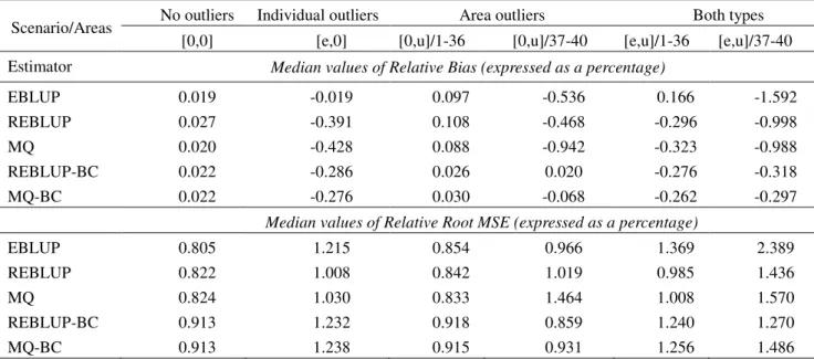
The performance of these estimators across the different areas and simulations is assessed by computing the median values of their area specific relative bias and relative root mean squared error, where the relative bias of an estimator ˆy_i for the actual mean y_i of area i is the average across simulations of the errors ˆy_i−y_i divided by the corresponding average value of y_i, and its relative root mean squared error is the square root of the average across simulations of the squares of these errors, again divided by the average value of y_i. Table 1 presents these median values for the different simulation scenarios and different estimators.

The relative bias results set out in Table 1 confirm our expectations regarding the behaviour of the projective estimators (EBLUP, REBLUP and MQ) and the bias-corrected predictive estimators (REBLUP-BC and MQ-(REBLUP-BC). The former are more biased than the latter (see scenarios with area and individual outliers) as a consequence of their implicit assumption that although outlier variances may be inflated relative to non-outliers, outlier effects still have zero expectation. This increase in bias is most pronounced when there are outliers in the area effects, which is not unexpected since that is when area means are most affected by the

presence of outliers in the population data. Turning to the median RRMSE results, we see that claims in the literature (e.g. Chambers and Tzavidis, 2006) about the superior outlier robustness of MQ compared with the EBLUP certainly hold true – provided the outliers are in individual effects. If there are outliers in area effects, then MQ appears to offer no extra protection compared to the EBLUP, and in fact performs worse, mainly due to its sharply increasing bias in this situation. Similarly, when we compare the EBLUP and the REBLUP we see that if outliers are associated with individual effects, then the REBLUP offers better RRMSE performance than the EBLUP. However, the gap between these two estimators narrows considerably when outliers are associated with area effects. In contrast, the two bias-corrected predictive estimators seem relatively robust in terms of RRMSE performance. Nevertheless, due to the increased variability as a consequence of their bias corrections, both BC estimators are not as efficient as the projective estimators when outliers are associated with individual effects, but both also do not fail when there are outliers in the area effects. Finally, the REBLUP-BC estimator appears to be performing better than the MQ-BC estimator for those scenarios where the use of predictive estimators offers gains.

We now examine the performance of the different MSE estimators. Here, we are mainly interested in the performance of alternative MSE estimators for estimating the MSE of the robust predictive estimators. However, we do also comment on the performance of the different MSE estimators when used for estimating the MSE of projective estimators under a range of scenarios.

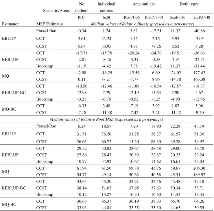
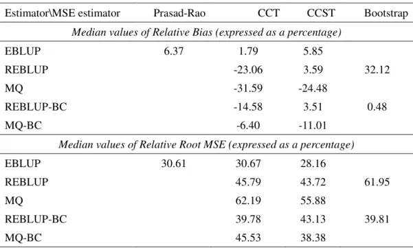
MSE estimation for the REBLUP and REBLUP-BC is implemented via the pseudo-linearization MSE estimator (23) (hereafter CCT) and via the linearization-based MSE estimators (34) and (38) (hereafter CCST). For the MQ and the MQ-BC the MSE estimators (A5) and (A7), which correspond to the CCST (see the Appendix for details), and the CCT are used (see Chambers et al. 2009 for details). For the REBLUP we further used the bootstrap procedure proposed by Sinha and Rao (2009), which is implemented by generating 100 bootstrap samples in each Monte Carlo run. Finally, the MSE of the EBLUP is estimated by using the Prasad-Rao (PR) estimator, but in addition we also evaluate the performance of the CCT and the CCST, obtained as a special case of (34), for estimating the MSE of this estimator. The results of the MSE estimators for each scenario and for each estimator are shown in Table 2 where we report the median values of their area specific relative bias and the relative root mean squared error.

We start first by evaluating the performance of the MSE estimators we proposed in this paper (CCT and CCST) for estimating the MSE of the robust predictive estimators REBLUP-BC and MQ-BC. We note while for the REBLUP-BC the CCST has a somewhat better performance, for the MQ-BC the CCT performs better in terms of bias. Although the RRMSEs of both MSE estimators have similar orders of magnitude, it appears that the CCST is less stable than the CCT when used to estimate the MSE of the REBLUP-BC but the reverse is true for the estimation of the MSE of the MQ-BC. Perhaps an improvement in the MSE estimation of the REBLUP-BC can be offered by using the parametric bootstrap MSE proposed by Sinha and Rao (2009). This estimator has an advantage both in terms of relative bias and RRMSE. However, for the case of the MQ-BC our only options are currently the CCT and CCST estimators.

Turning now to MSE estimation for the robust projective estimators we note the following. For the REBLUP estimator the parametric bootstrap MSE provides a very good approximation to the true MSE. Having said this, the CCST also provides a good alternative in this case. For example, in the case of outliers both at area level and at individual level the CCST records the lowest relative bias and the lowest RRMSE. For the MQ estimator the CCST estimator performs better than the CCT estimator. However, for the scenario with outliers at both the area and the unit level we observe that both CCT and CCST estimator record very high relative biases. Nevertheless, in the case of this scenario we should use a robust projective estimator in which case both the bootstrap or the CCST MSE estimators perform well. For the case of the EBLUP estimator, the PR estimator performs, as expected, well in the [0,0] scenario and also records small relative bias for some of the scenarios with outliers. The PR MSE estimator is also more stable than the CCT and the CCST for almost all scenarios. The CCT estimator has an impressively small relative bias for all scenarios. However, as pointed out by Chambers et al. (2009), the bias robustness of this MSE estimator comes at the price of high variability especially in the case of very small area sample sizes. Finally, the CCST performs worse in terms of relative bias but is more stable than the CCT.

6. Design-Based Simulation

Design-based simulations complement model-based simulations for SAE since they allow us to evaluate the performance of SAE methods in the context of a real population and realistic sampling methods where we do

not know the precise source of contamination. From a finite population perspective we believe that this type of simulation constitutes a more practical and appropriate representation of the SAE problem. Furthermore, it provides a good illustration of why a focus on conditional MSE is likely to be closer to the MSE of interest for analysts using small area methods.

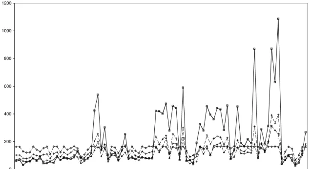
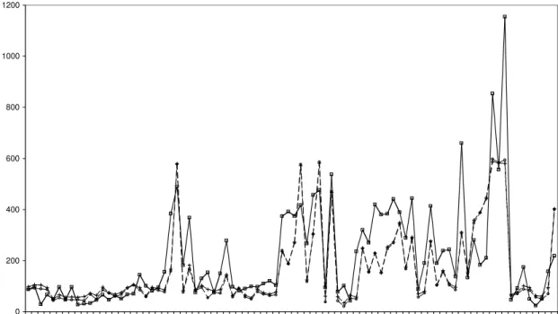
The population underpinning the design-based simulation is based on a data set obtained under the Environmental Monitoring and Assessment Program (EMAP) of the U.S. Environmental Protection Agency. The background to this data set is that between 1991 and 1995 EMAP conducted a survey of lakes in the North-Eastern states of the U.S. The data collected in this survey consists of 551 measurements from a sample of 334 of the 21,026 lakes located in this area. The lakes making up this population are grouped into 113 8-digit Hydrologic Unit Codes (HUCs), of which 64 contained less than 5 observations and 27 did not have any observations. In our simulation, we defined HUCs as the small areas of interest, with lakes grouped within HUCs. The variable of interest is Acid Neutralizing Capacity (ANC), an indicator of the acidification risk of water bodies. A total of 1000 independent random samples of lake locations are then taken from the population of 21,026 lake locations by randomly selecting locations in the 86 HUCs that contained EMAP sampled lakes, with sample sizes in these HUCs set to the greater of five and the original EMAP sample size. A two-level (level 1 is the lake and level 2 is the HUC) mixed model has been fitted to the synthetic population data. The Shapiro-Wilk normality test, whic