MPRA
Munich Personal RePEc Archive
Spurious Regression
Daniel Ventosa-Santaul`
aria
Escuela de Econom´ıa, Universidad de Guanajuato.
2008
Online at
http://mpra.ub.uni-muenchen.de/59008/
S
PURIOUS
R
EGRESSION
Daniel Ventosa-Santaul`aria
∗Abstract
The spurious regression phenomenon in Least Squares occurs for a wide range of Data Generating Processes, such as driftless unit roots, unit roots with drift, long memory, trend and broken-trend stationarity. Indeed, spurious regressions have played a fundamental role in the building of modern time series econome-trics and have revolutionized many of the procedures used in applied macroecono-mics. Spin-offs from this research range from unit-root tests to cointegration and error-correction models. This paper provides an overview of results about spurious regression, pulled from disperse sources, and explains their implications.
Keywords: Spurious Regression, Stationarity, Unit Root, Long Memory JEL Classification: C10, C12, C13, C22.
Introduction
During the last 30 years econometric theory has undergone a revolution. In the late seventies, economists and econometricians recognized that insufficient attention was being paid to trending mechanisms and that, in fact, most macroeconomic variables were probably nonstationary. Such an appraisal gave rise to an extraordinary deve-lopment that substantially modified the way empirical studies in time-series econo-metrics are carried out. Research in nonstationarity has advanced significantly since the early important papers, such as Granger and Newbold (1974), Davidson, Hendry, Srba, and Yeo (1978), Hendry and Mizon (1978), Plosser and Schwert (1978) Bhatta-charya, Gupta, and Waymire (1983) and Phillips (1986). Nelson and Plosser (1982) asserted that many relevant U.S. macroeconomic time series were governed by a unit
∗Departamento de Economia y Finanzas, Universidad de Guanajuato. Address: DCEA-Campus Marfil
root (a random trending mechanism), based on Dickey and Fuller’s (1979) Unit-root test. Several years later, Perron (1989) argued that the trending mechanism in macro variables was deterministic in nature (with some transcendent structural breaks). The debate continues between ’unit rooters’ and ’deterministic trenders’, though there is very general consensus as to the presence of a trending mechanism in the levels of most macroeconomic series. In the words of Durlauf and Phillips (1988):
“Traditional Analyses of Economic time series frequently rely on the assumption that the time series in question are stationary, ergodic processes[. . .]. However, the assum-ptions of the traditional theory do not provide much solace to the empirical worker. Even casual examination of such time series as GNP reveals that the series do not possess constant means”.
Econometrics should work hand-in-hand with economic theory by providing it with the tools it requires to understand economic activity. The modeling of such mechanisms is thus a major goal of time series econometrics.1 Spurious regression can be consi-dered as having played a fundamental role in this development. To understand it, we paraphrase Granger, Hyung, and Jeon (2001), who provide an illuminating definition [Phillips (1986) showed analytically that, when regressing two independent stochastic trends, the estimates of the regression coefficient do not converge to their real value of zero.2 Phillips’s (1986) results are detailed in a simple case in Appendix A]:
“A spurious regression occurs when a pair of independent series, but with strong tem-poral properties, is found apparently to be related according to standard inference in a Least Squares regression”.
Phillips (1998) presented a counterargument on the usefulness of spurious regression: trend specifications are just coordinate systems for representing behavior over time. Phillips argues that even if the series are statistically independent, when they include a trending mechanism in their DGP, they admit a regression representation (even in the absence of cointegration). This is in sharp contrast to the usual concept of
spu-rious regression. We usually conceive this phenomenon as the statistical identifica-tion of a commonality of trending mechanisms. Phillips ventures that such results–the ’spurious’–constitute an adequate representation of the data. His main result applies for regressions among stochastically trended series on time polynomials as well as regres-sions among independent random walks. Phillips (1998) proves that Brownian motions can be represented by deterministic functions of time with random coefficients. Given that standardized discrete time series with a unit root (hereinafter UR) converge wea-kly to Brownian motion processes, it is argued that deterministic time functions may be used to model them. Such representations include polynomial trends, trend breaks as well as sinusoidal trends; it is also proved that a stochastic process can represent an arbitrary deterministic function on a particular interval, so a regression of a UR process on an independent UR process is thus also a valid representation of the data. In both ca-ses, the t-statistics diverge at rateT12, which is consistent since such parameterization
reflects a partial–though correct–specification of the DGP. One of the most significant conclusions of Phillips concerns the long-standing debate of UR versus Trend Statio-narity. To quote Phillips:
“[. . .]Our results show that such specifications [Trend stationary processes] are not, in fact, really alternatives to a UR model at all. Since the UR processes have limiting representations entirely in terms of these functions (deterministic), it is apparent that we can mistakenly ’reject’ a UR model in favor of a trend ’alternative’ when in fact that alternative model is nothing other than an alternate representation of the UR process itself.’
This perspective has the virtue of allowing variables with different trending mecha-nism (deterministic or stochastic) to be related without being limited to the somewhat restrictive case of cointegration. Phillips advances this as an appropriate approach to study stochastically unbalanced relationships such as the ones that may arise between variables such as interest rates, inflation, money stock and GDP [for further detail, see
Phillips (2003)].
To the best of our knowledge, little has been done in the way of bringing the most important works in this field together, treating them in any kind of standardized way, making connections between them, and of any real study of the profound implications for economics they might indicate. This article aims to rectify this situation.
1
Appraisal of the spurious phenomenon
Much progress has been made with Least Squares statistical inference since it was first proposed more than two centuries ago as a means of estimating the course of comets (Legendre 1805). Theoretical developments in econometrics address the non-experimental nature of economic data sets. Least Squares (LS) offers a trade-off bet-ween simplicity and powerful inference. Nevertheless, LS has certain limitations, such as potential confusion between correlation and causality, and used unwisely may pro-duce misleading evidence. Statisticians and econometricians had been aware of the ”spurious phenomenon” since Yule (1897) and Pearson (1897) [for excellent reviews of these works, see Hendry and Morgan (1995) and Aldrich (1995)]. These results led to the common expertise in the time-series field that indicated the need to differentiate potentially nonstationary series when using these to run regressions or detrending these by fitting trend lines estimated with LS. See Morgan (1990).
There are many examples of spurious regression. Some of these are commented on in Phillips (1998), where we discover the implausible relationship between ‘the number of ordained ministers and the rate of alcoholism in Great Britain in the nineteenth century’; the equally ‘remarkable relationship’ presented in Yule (1926) concerning the ’proportion of Church of England marriages to all marriages and the mortality rate over the period 1866-1911’; the ‘strange relationship’ between price level and cumulative rainfall in the UK, which was advanced as a curious alternative version of quantitative theory by Hendry (1980). Plosser and Schwert (1978) presented another example of
nonsense correlation when they proposed their quantity theory of sunspots. The main argument is that the log of nominal income can be explained by way of the log of accumulative sunspots. Not only did they find statistically significant estimates, but the goodness of fit, measured with theR2, is quite high: 0.82.3 Granger and Newbold
(1974) computed a Monte Carlo Experiment where a number of regressions, specified as equation (1), were run using simulated variables, each perfectly independent of the others.
yt = α+βxt+ut (1)
wheret= 1, . . . , T, beingTthe sample size. The variablesxtandytare independent.
Under standard regularity conditions, LS delivers no evidence of a linear relationship betweeny andx. In particular,βˆshould be statistically equal to zero. Nevertheless, Granger and Newbold’s (1974) they were generated asI(1)processes,4usually referred to as random walks, that is, UR processes, but found estimated parameters statistically different from zero, with its associated t-ratiotβˆ =
ˆ
β
ˆ
σβˆ, unusually high.
5 Phillips
(1986) provided a theoretical framework that explained the causes of the phenomenon of spurious regression. In short, it is fair to say that standard LS inference can only be drawn when the variables are stationary. Even with stationary but highly persistent variables, spurious regression can occur when the standard errors used in the t-ratio are inconsistent. Ferson, Sarkissian, and Simin (2003) provide examples in financial economics. One extremely important exception to this is the case of cointegration. Even if the series are stochastically trending, when the trend is common to both series the LS regression then works particularly well in the sense that estimates converge in probability to their true value at a rate faster thanT, but have a nonstandard distribution (Stock 1987).
2
Data Generating Processes
Research on spurious regression has been making use of increasingly complex Data Generating Processes (DGPs). Table (1) provides a summary of those appearing in this survey: # Name Model 1 M A(qw)or wt=Piq=1w Θiwǫwt−ior AR(pw) wt=Pip=1w φwiwt−i+ǫwt(stationary) 2 I(0) wt=µw+uwt 3 I(0) +br wt=µw+PiN=1wθiwDUiwt+uwt 4 T S wt=µw+βwt+uwt 5 T S+br wt=µw+PNwi=1θiwDUiwt+βwt+PMwi=1γiwDTiwt+uwt 6 I(1) ∆wt=uwt 7 I(1) +dr ∆wt=µw+uwt 8 I(1) +dr+br ∆wt=µw+PNi=1wθiwDUiwt+uwt 9 I(k) ∆kw t=uwtfork= 2,3, . . . 10 F I(d) (1−L)dwt=uwtford∈ 0,12 11 F I(1 +d) ∆wt=uwtwith(1−L)duwt=ǫwtford∈ 0,32
Table 1: The DGP’s for wt = xt, yt, zt. Note: T S, br and dr stand for
trend-stationarity, breaks, and drift, respectively.
whereuwtare independent innovations obeying Assumption 1 in Phillips (1986),ǫwt
is an iid white noise with mean zero and varianceσ2
ǫ, andDUiwt,DTiwtare dummy
variables allowing changes in the trend’s level and slope respectively, that is,DUiwt=
1(t > Tbiw)andDTiwt= (t−Tbiw)1(t > Tbiw), where1(·)is the indicator function,
andTbiw is the unknown date of thei
thbreak inw. We denote the break fraction as
λiw = (Tbiw/T) ∈ (0,1),where T is the sample size;d ∈ −
1 2, 3 2 . Only DGPs1,
2and10(ford < 0.5) satisfy the weak stationarity definition. The remaining DGPs generate nonstationary series.6F Iprocesses deserve further discussion; contrary to re-gularARM A(p, q)processes–made popular by Box and Jenkins in the 1970s–such as DGP 1, whose autocorrelation function decays at an exponential rate (short memory),
memory).
There are a number of empirical examples in time series in which dependence falls slowly across time. This phenomenon, known as Long Memory or Long-Range de-pendence, was observed in geophysical data, such as river flow data (Hurst 1951) and in climatological series (Hipel and McLeod 1978), as well as in economic time series (Adelman 1965). In three important papers (Granger 1980, Granger and Joyeux 1980, Hosking 1981), the authors extended these processes to provide more flexible low-frequency or Long Memory behavior by consideringI(d)processes with non-integer values ofd. As pointed out by Granger and Joyeux (1980), “It was standard procedure
to consider differencing time series to achieve stationarity”–thus obtaining a form of
the series that can be identified as anARM Amodel–however, “Some econometricians
were reluctant to this technique, believing that they may be losing information, by zap-ping out the low frequency components.” But using infinite variance series without
differencing them was also a source of difficulties at that time. Fractional integration encompassesARM Amodels ford= 0, andARIM Amodels ford= 1. The process is stationary and ergodic whend∈ −1
2, 1 2
; nonstationary but mean-reverting7when
1
2 < d <1, and nonstationary and mean averting whend≥1.
Mean stationary processes (DGPs 2 and 3) have been used to model the behavior of real exchange rates, unemployment rates, current account, and several great ratios, such as the output-capital ratio and the consumption-income ratio. Unemployment has also been conceived as a nonstationary fractionally integrated process (Arino and Marmol 2004). Some examples can be found in Perron and Vogelsang (1992), Wu (2000), Wu, Chen, and Lee (2001) and D’Adda and Scorcu (2003). Trend Stationarity andI(2)
processes (DGPs 4 and 9, respectively) have been used to model growing variables, real and nominal, such as output, consumption and prices; several macro variables have been conceived as DGPs 5, 6, and 7 (Perron 1989, Perron 1997, Lumsdaine and Papell 1997, Mehl 2000). Variables identified asI(2) processes can also be found
in Juselius (1996), Juselius (1999), Haldrup (1998), Muscatelli and Spinelli (2000), Coenen and Vega (2001), and Nielsen (2002). In Table (11) of appendix B, a few more examples are provided, in which the link between time-series econometrics and important economic issues is acknowledged.
3
Spurious regression since the roaring twenties
We now begin our survey of the development of the theory of spurious regression. The related literature is vast, for which reason we focus mainly on a limited selection of articles which, in our view, are particularly representative.8 Unless otherwise
speci-fied, the regression specification for which all asymptotics are presented is hereinafter expression (1). We focus mainly on on the rate of divergence of the relevant t-ratios and let aside in most cases the asymptotic distributions that would be obtained had the statistics being correctly normalized. This is so because such distributions do have nuisance parameters that prevent one from making use of these to do correct inference; moreover, practitioners cannot be aware a priori of the adequate normalization. Ho-wever, in some cases (Kim, Lee, and Newbold 2004, Sun 2004, Moon, Rubia, and Valkanov 2006) the asymptotic distributions are important because of the relevance for practitioners.9
3.1
Yule’s experiment
Spurious correlation was evidenced by Yule (1926) in a computerless Monte Carlo experiment. Shuffling decks of playing cards, Yule obtained independent series of ran-dom numbers. In fact, Yule generated independentI(0),I(1), and I(2)series and computed correlation coefficients amongst them. Such correlation coefficients provi-ded correct inference when usingI(0)series, but became nonsensical when the order of integration of the variables was higher. With independentI(0)variables the correlation coefficient remained close to zero. The same estimate achieved usingI(1)independent
variables no longer worked; many times it was close to unity, resulting in what we now refer to as a spurious correlation. If variables wereI(2), the most probable outcome was actually a correlation coefficient of close to1: the spurious phenomenon was even stronger.
3.2
Reappraisal in the seventies: spurious Least Squares
Throughout most of the past century, it was commonly recommended to first-difference the series if these seemed to have a trending mechanism. However, not every econo-metrician was in agreement with such a method because, it was argued, differencing causes losses in the information contained in the original series. A profound reapprai-sal of this issue began with Granger and Newbold’s (1974) article, which allowed the spurious regression in Least squares estimators to be identified. The Monte Carlo ex-periment described above revealed, among other things, that highR2and low
Durbin-Watson statistics (hereinafterDW) should be considered as a sign of misspecification. They also pointed out, comparing the outcome of simulation with many results in ap-plied econometrics, that problems of misspecification seemed to be widespread. It was proposed that first-differenced series be used, although the authors warned about the risks of catch-all solutions; their results may be considered as the seed of many fruitful extensions in time series econometrics.
3.3
Theory at last: asymptotics in nonsensical regressions
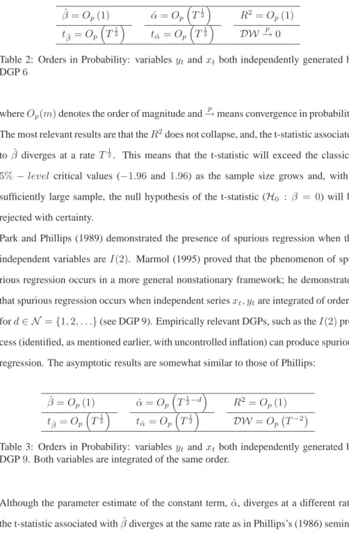
Phillips (1986) proposed the theoretical framework necessary to allow an understan-ding of Granger and Newbold’s earlier results and provided a first insight into the phe-nomenon of spurious regression. His development set the groundwork for the spurious regression literature in econometrics. Whilst Granger and Newbold used ani.i.d.noise in their simulations , Phillips allowed a flexible autocorrelation structure, as well as some degree of heterogeneity. He then proved that, when specification (1) is estimated
the following asymptotics are obtained: ˆ β=Op(1) αˆ=Op T12 R2=O p(1) tβˆ=Op T12 tαˆ=Op T12 DW→p 0
Table 2: Orders in Probability: variablesytandxtboth independently generated by
DGP6
whereOp(m)denotes the order of magnitude and p
→means convergence in probability. The most relevant results are that theR2does not collapse, and, the t-statistic associated
toβˆ diverges at a rateT12. This means that the t-statistic will exceed the classical
5%−level critical values (−1.96 and1.96) as the sample size grows and, with a sufficiently large sample, the null hypothesis of the t-statistic (H0 : β = 0) will be
rejected with certainty.
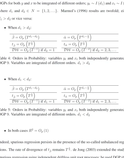
Park and Phillips (1989) demonstrated the presence of spurious regression when the independent variables areI(2). Marmol (1995) proved that the phenomenon of spu-rious regression occurs in a more general nonstationary framework; he demonstrated that spurious regression occurs when independent seriesxt, ytare integrated of orderd
ford∈ N ={1,2, . . .}(see DGP 9). Empirically relevant DGPs, such as theI(2) pro-cess (identified, as mentioned earlier, with uncontrolled inflation) can produce spurious regression. The asymptotic results are somewhat similar to those of Phillips:
ˆ β=Op(1) αˆ =Op T12−d R2=O p(1) tβˆ=Op T12 tαˆ=Op T12 DW=Op T−2
Table 3: Orders in Probability: variablesytandxtboth independently generated by
DGP9. Both variables are integrated of the same order.
Although the parameter estimate of the constant term,αˆ, diverges at a different rate, the t-statistic associated withβˆdiverges at the same rate as in Phillips’s (1986) seminal
work, i.e.Op
T12
.
One limitation of Marmol’s (1995) results is that both the dependent and the indepen-dent variables share the same order of integration. Banerjee, Dolado, Galbraith, and Hendry (1993), provided Monte Carlo evidence of spurious regression when the order of integration of each variable is different. Marmol (1996), later allowed the relevant DGPs for bothyandxto be integrated of different orders;yt∼I(d1)andxt∼I(d2)
where d1 and d2 ∈ N = {1,2, . . .}. Marmol’s (1996) results are twofold; either
d1> d2or vice versa: • Whend1> d2: ˆ β=Op Td1−d2 ˆ α=Op Td1− 1 2 tβˆ=Op T12 tαˆ=Op T12 DW=Op T−1ifd2= 1 DW=Op T−2ifd2= 2,3, . . .
Table 4: Orders in Probability: variablesytandxtboth independently generated by
DGP9. Variables are integrated of different orders.d1> d2
• Whend1< d2: ˆ β=Op Td1−d2 αˆ=Op Td1−12 tβˆ=Op T12 tαˆ=Op T12 DW=Op T−1 ifd1= 1 DW=Op T−2 ifd1= 2,3, . . .
Table 5: Orders in Probability: variablesytandxtboth independently generated by
DGP9. Variables are integrated of different orders.d1< d2
• In both casesR2=O
p(1)
Indeed, spurious regression persists in the presence of the so-called unbalanced regres-sions. The rate of divergence oftβˆremainsT
1
2. de Jong (2003) extended the study of
spurious regression using independent driftless unit root processes; he used DGP (6) to generate the series and ran the following specification, which operates with logarithmic
transformation of both variables–a direction which has proved extremely relevant for empirical purposes:10
ln (yt) = α+βln (xt) +ut
de Jong discovered similar results to previous works, i.e. βˆ = Op(1) and tβˆ = Op
T12
.
Entorf (1997) made a slight-and yet, fundamental-modification to the Phillips’ DGPs by adding a drift (DGP 7).11 Amongst the most relevant consequences of such drift is
the fact that there is not only a stochastic trend but also a deterministic one. In the long run, the deterministic trend dominates the stochastic (see Appendix C). The asymptotic results of estimating equation (1) using independent variables generated by DGP 7 are:
tβˆ=Op(T) tαˆ=Op T12 1−R2=O p T−1 DW=Op T−1
Table 6: Orders in Probability: variablesytandxtboth independently generated by
DGP7.
Note thattβˆgrows at rateTinstead ofT
1
2, contrary to the results presented so far, due
to the presence of a deterministic trend.
3.4
Spurious regression and long memory: an unforgettable
exten-sion
Among the first papers to deal with spurious regression in econometrics12 using long memory processes are those of Cappuccio and Lubian (1997) and Marmol (1998). The authors use the nonstationary fractionally-integrated processes specified in DGP 11. Under these conditions, the asymptotics of an LS regression as specified in expression (1) are as follows:13
ˆ β=Op(1) tβˆ=Op T12 R2=O p(1) DW=Op T−(1+2d)
Table 7: Orders in Probability: variablesytandxtboth independently generated by
DGP11. The variables are integrated of the same order.
Note that as most of the previous cases the t-statistic ofβˆdiverges at rateT12. The
main difference lies in theDW, the rate of divergence of which varies according to the degree of long memory, measured byd. These results can be understood as an argu-ment against the usefulness of the ‘rule-of-thumb’; a regression was usually considered spurious whenR2 >DW. However, when long memory is present in the variables,
the regression may well be spurious even ifR2<DW. It is worth mentioning that the
fractional integration parameter,d, is the same in both variables. This ‘shortcoming’ is fixed by Tsay and Chung (2000), who used a manifold approach. They used two DGPs (No 10 and 11) and then combined these in a simple regression. Thus, there are four fractionally-integrated processes, two stationary,[F I(d1) andF I(d2) with
di∈ 0,12
, and two nonstationary,[F I(di+ 1) for di ∈ 12,32
. The authors then studied several specifications using six DGPs. The first four are used in the estimation of specification (1) whilst the remaining two estimateyt=α+δt+ut:
1. yt∼F I(1 +d1)andxt∼F I(1 +d2),14 2. yt∼F I(d1)andxt∼F I(d2)whered1+d2>12, 3. yt∼F I(1 +d1)andxt∼F I(d2)whered2>12, 4. yt∼F I(d1)andxt∼F I(1 +d2)whered1>12, 5. yt∼F I(1 +d1)whered1>0, 6. yt∼F I(d1)whered1>0.
We can summarize the results by stating thattβˆ =Op(Tr)where0 < r < 1which
means that the t-ratio always diverges; the divergence rate,r, is,T12,Td1+d2−12,Td2,
Special attention should be given to the Durbin-Watson statistic, which collapses to zero (as usual) except in the second case, whereDW = Op(1)and hence does not
converge to zero as it does elsewhere. This also could be interpreted as an important indication of the need for caution when using the rule-of-thumb, which states that when
R2 > DW there may be spurious regression. As in Cappuccio and Lubian (1997), there is evidence that the rule-of-thumb may be a dangerous tool. Another important result appears when we compare model 1 and model 2. The reader may notice that the variables used in the second model are merely the first differences of those used in the first. What is surprising is that the spurious regression persists after the variables have been differenced.15 This goes against fifty years of tradition (differencing is used
to deal with spurious regression16). Tsay and Chung (2000) actually go further by
suggesting that the spurious phenomenon is due to the long memory properties of the series and not to the presence of unit roots.17 Sun (2006) shows that spurious regression can occur between two stationary generalized fractional processes, as long as their generalized fractional differencing parameters sum up to a value greater than 12 and their spectral densities have poles at the same location.
3.5
Spurious regression with stationary series: size-matters
Granger, Hyung, and Jeon (2001) show, both through Monte Carlo experiments and theoretically that the spurious regression phenomenon may occur amongst independent stationary series.18 Two independentAR(1)series (see DGP 2 withPw= 1) were run
together to estimate regression (1), resulting in a rejection rate of the t-statistic greater than the expected 5%. Granger, Hyung, and Jeon (2001) provide a theoretical proof of why this happens (although the variance of the estimates does not diverge, it may not be unity, depending on the values of the DGP’s parameters).19
These results are extended to long-spanM Aprocesses (see DGP 1). Curiously, the spurious regression does not depend on the sample size, but rather on theM Aspan
parameter,qw. What is interesting about this result is the fact that it better explains
the spurious regression phenomenon in small-sized samples. This would complete the theoretical framework necessary to allow an understanding of the Monte Carlo results of Granger and Newbold (1974) and Ferson, Sarkissian, and Simin (2003)
Granger, Hyung, and Jeon’s (2001) results differ from all others, the effect being dis-cussed is not not an asymptotic phenomenon but rather a size distortion. Size distor-tions arise because standardizing a test statistic is difficult unless the exact form of the spectral density of the residuals is known. The intuition behind the spurious regression phenomenon is thus, different from the one that underlies all other results.
Mikosch and de Vries (2006) provide an alternative theory to explain spurious-type behavior akin to the financial risk measurement literature.20 In the words of Mikosch
and de Vries (2006):
“Estimators of the coefficients in equations of regression type which involve financial data are often found to vary considerably across different samples. This observation pertains to finance models like the CAPM beta regression, the forward premium equa-tion and the yield curve regression. In economics, macro models like the monetary model of the foreign exchange rate often yield regression coefficients which signifi-cantly deviate from the unitary coefficient on money which is based on the theoretical assumption that money is neutral.”.
Mikosch and de Vries (2006) prove that, when the distribution of the innovations is heavy tailed, that is, when there is a departure from the normality assumption usually made, using standard statistical tools (such as LS, for example) can be misleading.21
3.6
The last newcomer: Trend Stationarity
Hassler (2000) studied the spurious regression phenomenon from a different perspec-tive. He considered the possibility of spurious regression when the variables do have a deterministic trend component (what we have defined earlier as trend stationarity [DGP
4]). Thus, there are two independent nonstationary variables. Hassler’s (2000) results, as with those of Kim, Lee, and Newbold (2004), who worked with the same DGPs, are as follows: tβˆ=Op T32 β=Op(1) T2 1−R2 p →0
Table 8: Orders in Probability: variablesytandxtboth independently generated by
DGP4.
In addition, Kim, Lee, and Newbold (2004) proved that when one of the deterministic trend components is taken out (that is, eitherβy = 0andβx6= 0or vice versa), the
t-ratios converge to centered normal distribution, although its variance is not unity, which may provoke spurious rejection of the null hypothesis that the parameter is zero. That means that running a trend stationary variable (DGP 4) on a mean stationary variable (DGP 2) or vice versa lessens the ”spuriosity” in the regression. The authors also generated independent series with the DGP (4), as did Entorf (1997), although they ran a different specification:
yt = α+βxt+δt+ut (2)
The asymptotics provided in Kim, Lee, and Newbold (2003) only concernβˆandtβˆ. We
computed the orders in probability of the other two parameters, given their relevance. We included in Appendix D a guide on how to obtain these asymptotics:
ˆ α=Op(1) tˆα=Op T12 ˆ β =Op T−12 tβˆ=Op(1) ˆ δ=Op(1) tˆδ =Op T12
Table 9: Orders in Probability: variablesytandxtboth independently generated by
It should be noted that the t-ratio converges to a normal distribution. However, since the variance is not unity, spurious regression may well be still present.
A relevant extension of Hassler (2000) and Kim, Lee, and Newbold (2004) was provi-ded by Noriega and Ventosa-Santaul`aria (2006b) where (possibly multiple) structural breaks are added to the Trend Stationary DGP, i.e. DGP 5. Adding breaks to the speci-fication of the DGPs makes the divergence rate of the t-statistic associated withβˆreturn to the usualT12 ‘norm’. They also proved that adding a deterministic trend into the
re-gression specification (see equation 2) does not prevent the phenomenon of spurious regression;tˆδ remainsOp
T12
. In an effort to unify the related literature, Noriega and Ventosa-Santaul`aria (2007) filled a number of gaps until then unaddressed. They studied several previously overlooked combinations of DGPs and summarized most of the others’ results. DGPs 2-9 may indistinctly generatexand/ory.22 In fact, amongst the new possible combinations, the divergence rate oftβˆ usually remainsT
1 2. The
combination of a Trend Stationary and anI(1) plus drift stands out since the diver-gence rate of the t-ratio isT rather thanT12 as in Kim, Lee, and Newbold (2004),
although this result should have been anticipated given the asymptotic dominance of the deterministic trend over the stochastic. This combination is thus clearly linked to Entorf’s (1997) results.
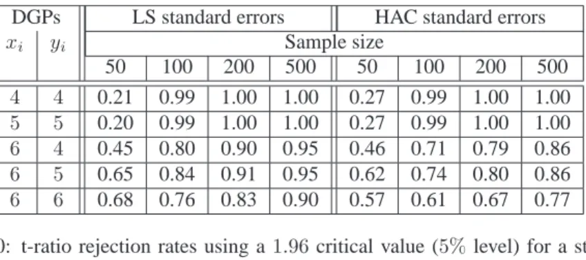
Granger, Hyung, and Jeon (2001) showed that the use of an Heteroskedasticity and Autocovariance covariance matrix diminishes size distortions in some cases but their Monte Carlo evidence also showed that this is true only when the sample size is large (greater than500). The use of HAC standard errors23 when the DGPs are stationary or have a deterministic trend is not so obvious. We performed a simple simulation to support this view (see table 10). The variablesxandy are independently generated either by DGP (4), (5), or (6). Lag selection was done as in Granger, Hyung, and Jeon (2001), that is, using the formula: l = integerh4 (T /100)1/4i. Simulation results show that size distortions are less severe when HAC is used, but remain extremely
high (perhaps results would improve further if the data could follow a pre-whitening procedure).
DGPs LS standard errors HAC standard errors
xi yi Sample size 50 100 200 500 50 100 200 500 4 4 0.21 0.99 1.00 1.00 0.27 0.99 1.00 1.00 5 5 0.20 0.99 1.00 1.00 0.27 0.99 1.00 1.00 6 4 0.45 0.80 0.90 0.95 0.46 0.71 0.79 0.86 6 5 0.65 0.84 0.91 0.95 0.62 0.74 0.80 0.86 6 6 0.68 0.76 0.83 0.90 0.57 0.61 0.67 0.77
Table 10: t-ratio rejection rates using a1.96critical value (5%level) for a standard normal distribution: spurious regression using LS and HAC standard errors.
3.7
Next of kin: statistical tests, Long Horizon, and Instrumental
Variables
Not all work on the spurious phenomenon has been monopolized by the LS simple estimator. Stochastic trending mechanisms have been used in most of the studies, alt-hough some exceptions are presented at the end of this section. Equally relevant are the Instrumental Variables (IV) estimates, which have also been analyzed (Ventosa-Santaul`aria 2009).
Giles (2007) studied two important residual tests: the Jarque-Bera test [hereinafterJ B; see Jarque and Bera (1980)] and the Breusch-Pagan-Godfrey test (Breusch and Pagan 1980, Godfrey 1988), used to test for normality and autocorrelation/heteroskedasticity evidence in the residuals of an LS regression, respectively; he used independent driftless random walks (DGP 6) and proved that both statistics diverge at rateT, that is:
• Jarque-Bera test:J B=Op(T)
• Breusch-Pagan-Godfrey test: T·R2=O
p(T)
The null hypothesis of normality or serial independence/homoskedasticity will be even-tually rejected even if it is correct, given a large enough sample.24 Furthermore,
Ventosa-Santaul`aria and Vera-Vald´es (2008) studied the behavior of the classical Gran-ger-Causality test [see Granger (1969)], hereinafter GC. It is proved that the classical GC test fails to accept the null hypothesis of no GC between independent broken-trend (DGP 5) or broken-mean (DGP 3) processes whether the former series are differenced or not.
Kim, Lee, and Newbold (2005) study several important nonlinearity tests: the RESET test (Ramsey 1969), the McLeod and Li test (McLeod and Li 1983), the Keenan test (Keenan 1985), the Neural Network test (White 1989), White’s Information test (White 1992), and the Hamilton test (Hamilton 2000). All these tests were studied by way of finite-sample experiments using independent driftless random walks (see DGP 6). They also presented the asymptotics of the RESET and Keenan tests; both test-statistics are
Op(T), so the null of linearity is eventually rejected as the sample size grows. In the
same vein, Noriega and Ventosa-Santaul`aria (2006a) proved that, when the variables are generated independently by any combination of DGPs (3), (5), (7), and (8), the Engle and Granger cointegration-test spuriously rejects the null of no cointegration25
in an indeterminate number of cases since the relevant t-statistic isOp
T12
.26
Spurious regression has also been identified in the context of Long-Horizon (henceforth LH) regressions, which are used in situations where previous “short-term”27 studies
have failed. In fact, Valkanov’s (2003) insight is that rolling summations ofI(0) varia-bles, that is LH variavaria-bles, behave asymptotically asI(1)series. Hence, the theory of spurious regression between independentI(1)variables, discussed earlier, should give readers the intuition. Late eighties’ studies provided interesting results in economics and finance. As asserted by Valkanov (2003):
“The results[. . .]are based on long-horizon variables, where a long-horizon variable is obtained as a rolling sum of the original series. It is heuristically argued that long-run regressions produce more accurate results by strengthening the signal coming from the data, while eliminating the noise”.
More precisely, if the specification to be estimated is equation (1), a Long-Horizon “reinterpretation” is carried out with the building of partially aggregated variables. As usual, let,w = x, y, thenwk
t =
Pk−1
j=0wt+j. The LH regression specification can
usually be one of the following:
yk
t = α+βxkt +ut (3)
ykt = α+βxkt−k+ut
ykt = α+βxt+ut
Such specifications are used mostly in the estimation of the equity/dividend relations-hip and to test both the neutrality of money or the Fisher effect. Based upon the pre-vious specifications, Valkanov (2003) and Moon, Rubia, and Valkanov (2006) proved that this regression strategy also presents the spurious regression phenomenon. To do this, they let time overlap in the summations as a fixed fraction of the sample size,
k= [λ·T]whereλ∈[0,1]. Valkanov (2003) then defines the following DGP:
yt = βxt+uyt (4)
where (1−L)φ(L)xt = uxt. The variable xt follows an autoregressive process
whose highest root is unity whilst the rest, represented in the polynomialφ(L), is invertible. Letω = (uyt, uxt)′ be defined as a martingale difference sequence with
E(ωtω′t|ωt−1. . .) = σ211σ12;σ21σ222
and finite fourth moment. We could argue that, whenβ = 0, the t-ratio associated with its estimate should be small enough for the null hypothesis to be accepted. As in previous results, that does not happen;
tβˆ=Op
T12
. Valkanov (2003) and Moon, Rubia, and Valkanov (2006) suggest the use of a rescaled t-ratio, tβˆ
T12
. Although the limiting distribution of such t-statistic’s is neither normal nor pivotal, it can be easily simulated and hence used. Lee (2006) extends the results for fractionally integrated processes and finds that the t-ratio
asso-ciated withβˆin equation (3) diverges:tβˆ=Op
T12
.
Ventosa-Santaul`aria (2009) studies the asymptotics of Instrumental Variables (IV) using DGPs (5) and (7), not only forxandy, but also for a spurious and independent ins-trument. It is shown that the t-ratio still diverges at rateT12 which confirms the Monte
Carlo simulations carried out by Leybourne and Newbold (2003). This result can be also seen as a complement to those presented by Phillips and Hansen (1990) and Han-sen and Phillips (1990), in which the use of spurious instruments is proposed to im-prove the estimates whenever strong endogeneity is present betweenxand the residual term in cointegrated relationships.
Sun (2004) developed a convergent t-statistic for correcting the phenomenon of spu-rious regression. The new t-ratio is based on an estimate of the parameter variance made in the same manner as HAC standard errors. This t-statistic converges to a non-degenerate limiting distribution for many cases of spurious regression. He considered the regression between two independent nonstationaryI(d)processes withd > 12 as well as the regression between an independent nonstationaryI(d)process and a linear trend [see equation (5)]:
yt=α+δt+ut (5)
In previous studies, the presence of unit roots in the series generally produced aT12
divergent t-ratio. To avoid such divergence, Sun proposes a rescaling of the parameter estimate using a new standard error. The new Standard Error is computed in the same way HAC is. The main difference is that HAC estimates usually require a bandwidth or truncation lag. Sun suggests using the entire sample length:
ˆ σ2βˆ = T X t=1 (xt−x¯)2 !−1 ·TΩˆ · T X t=1 (xt−x¯)2 !−1
where ˆ Ω = T−1 X j=−T+1 κ j T ˆ Γ(j) ˆ Γ(j) = 1 T PT−j t=1 (xt+j−x¯) ˆut+juˆt(xt−x¯) f or j≥0 1 T PT t=−j+1(xt+j−x¯) ˆut+juˆt(xt−x¯) f or j <0
whereκis a kernel function that belongs to a class that ensures positive definitiveness. Whetherxt∼I(d)orxt=t, well-defined asymptotic distributions for the t-ratio are
provided.
4
What to do if one fears spurious regression
The spurious regression phenomenon pervades many subfields in time series analysis. It might be controlled by using correctly scaled t-ratios, as suggested earlier, but ha-ving a clear idea of what DGP best emulates the properties of the series (this could be labeled as DGPi-fication) would therefore be necessary (examples of this can be: (i) evidence of UR must be obtained before a cointegration analysis is undertaken; (ii) the nature of the trending mechanism should be identified prior to the application of a transformation intended to render stationary the series, and; (iii) a test such as Robin-son’s (1994) could be undertaken in order to identify long-memory behavior). This can be achieved by means of applying a battery of tests to our series. Such an approach is not exempted of failures. Many statistical tests are known to yield spurious evidence under specific circumstances (see the previous subsection). Nevertheless, pretesting the series remains an adequate strategy and allows the practitioner to be aware of the poten-cial difficulties he could face. In this section we include a short—and incomplete—list of tests that are employed in the DGPi-fication of the series:
means of Dickey-Fuller-type (DF) tests [see Dickey and Fuller (1979) and Di-ckey and Fuller (1981)]. The original DF test distinguishes between the null hypotheses of UR (DGPs 6 and 7) and the alternatives of stationarity (DGPs 1, 2 and 4). Other well-known UR tests are: (i) the KPSS test (Kwiatkowski, Phillips, Schmidt, and Shin 1992); (ii) the GLS-detrended DF test (Elliott, Rothenberg, and Stock 1996); (iii) the Phillips-Perron test (Phillips and Perron 1988), and; (iv) the Ng and Perron test (Ng and Perron 2001, Perron and Ng 1996).
2. The UR tests previously mentioned provide severely biased results under the hypothesis of trend-stationarity in the presence of structural breaks;28 several
alternatives are available. Perron (1989) suggested the use of a DF-type test with (point,level and trend) breaks specified in the auxiliary regression (see DGP 5); the break dates must be decided by the practitioner. Zivot and Andrews (1992) also proposed to modify the DF test in the same direction than Perron, only they allowed the break date to be endogenously specified; their test allows for a single break [see Lumsdaine and Papell (1997) for an extension that allows for two breaks] under the alternative hypothesis (DGP 5) and rules out the possibility of a break under the null hypothesis of UR (DGP 8); Carrion–i–Silvestre and Sans´o (2006) proposed a test where a break under the null hypothesis is taken into account.
3. Bai and Perron (1998) proposed a test to distinguish between DGPs 2 and 4 and DGPs 3 and 5. The test presupposes that the trending mechanism is exclusively deterministic.
4. Long-range dependence: many testing procedures are also available. R/S-type test [see Hurst (1951), Mandelbrot and Taqqu (1979) and Lo (1991)] are com-monly used to identify Long Memory (LM) against stationarity. However, Bhat-tacharya, Gupta, and Waymire (1983) proved that the classical R/S test may provide evidence of LM even if the series is stationary when the latter contains
a trending mechanism. Moreover, Mikosch and St˘aric˘a (2000) and Mikosch and St˘aric˘a (2004) proved that the sample autocorrelation function (sample ACF) can also be a misleading statistical tool when used to identify LM; stationary series that include a non-linear component might yield a sample ACF usually attributed to LM processes [see also Teverovsky and Taqqu (1997)]. Several Short memory processes may thus seem to behave as LM processes. This phenomenon can be labeled as spurious long memory (Mikosch and St˘aric˘a 2004).
5. Many other tests have been proposed to identify LM while they control for pos-sible non-linearities (structural breaks in the mean or the variance of the series). See Liu, Pan, and Hsueh (1993), Robinson (1994), Lobato and Robinson (1996), Giraitis, Kokoszka, and Leipus (2001), Giraitis, Kokoszka, Leipus, and Teys-siere (2003), Berkes, Horv´ath, Kokoszka, and Shao (2006), Zhang, Gabrys, and Kokoszka (2007), Aue, Horv´ath, Huˇskov´a, and Kokoszka (2008), and Jach and Kokoszka (2008).
Concluding remarks
Spurious regression can arise wherever a trending mechanism is present in the data. Even some stationary-autocorrelated processes cause spurious results.
Applied macroeconomists and financial experts have been steadily incorporating tech-nical advances in the analysis of the spurious regression, a phenomenon identified for many empirically-relevant Data Generating Processes. These include stationary pro-cesses withAR(or longM A) structure and/or level breaks; random walks (with or without drifts), trend stationarity (with possible level and trend breaks), long-memory processes (whether stationary or not) and so on. These processes have been associated with unemployment rates, price levels, real exchange rates, monetary aggregates, gross domestic product and various financial variables. The use of Least Squares with such
variables entails a high risk of obtaining a spurious relationship.
Differencing the series may not always prevent spurious estimates; nor should the
R2>DWrule-of-thumb be seen as an adequate rule to identify a spurious regression.
Cointegration analysis appears to better prevent non-sensical statistical relationships although, one should bear in mind Phillips’s (2003) and further study the statistical relationship at hand. Out-of-sample forecasting evaluation could be an option. Most macroeconomic variables are either nonstationary or very persistent. Pre-testing the variables in order to identify the nature of the trending mechanism arises as the gol-den rule to avoid non-sense regression. Once the DGP is correctly igol-dentified, spurious regression is “easier” to deal with.
Attaining a clear understanding of any problem is the first step toward finding its solu-tion.
References
ADELMAN, I. (1965): “Long Cycles: Fact or Artifact,” American Economic Review, 55, 444–463.
AGHION, P., ANDS. N. DURLAUF(2005): Handbook of Economic Growth, Volume
1A. North-Holland.
ALDRICH, J. (1995): “Correlations genuine and spurious in Pearson and Yule,”
Statis-tical Science, 10(4), 364–376.
ALOGOSKOUFIS, G., ANDR. SMITH(1991): “The Phillips Curve, The Persistence of Inflation, and the Lucas Critique: Evidence from Exchange-Rate Regimes,” The
American Economic Review, 81(5), 1254–1275.
ARINO, M., AND F. MARMOL (2004): “A permanent-transitory decomposition for ARFIMA processes,” Journal of Statistical Planning and Inference, 124, 87–97. AUE, A., L. HORVATH´ , M. HUSKOVˇ A´, AND P. KOKOSZKA (2008): “Testing for
changes in polynomial regression,” Bernoulli, 14(3), 637–660.
BAI, J.,ANDP. PERRON(1998): “Estimating and Testing Linear Models with Multiple
Structural Changes,” Econometrica, 66, 47–78.
BANERJEE, A., J. DOLADO, J. GALBRAITH, AND D. HENDRY (1993): Co-Integration, Error Correction, and the Econometric Analysis of Non-Stationary Data. Oxford University Press.
BARDSEN, G., E. JANSEN,ANDR. NYMOEN(2004): “Econometric Evaluation of the New Keynesian Phillips Curve,” Oxford Bulletin of Economics and Statistics, 66(s 1), 671–686.
BERKES, I., L. HORVATH´ , P. KOKOSZKA,ANDQ. SHAO(2006): “On discriminating between long-range dependence and changes in mean,” Annals of Statistics, 34(3), 1140–1165.
BERNARD, A., AND S. DURLAUF (1995): “Convergence in International Output,”
Journal of Applied Econometrics, 10(2), 97–108.
BERNARD, A.,ANDS. DURLAUF(1996): “Interpreting tests of the Convergence Hy-pothesis,” Journal of Econometrics, 71, 161–173.
BHATTACHARYA, R., V. GUPTA,ANDE. WAYMIRE(1983): “The Hurst effect under trends,” Journal of Applied Probability, pp. 649–662.
BREIDT, F., N. CRATO, ANDP. DELIMA(1998): “The detection and estimation of long memory in stochastic volatility,” Journal of Econometrics, 83(1-2), 325–348. BREUSCH, T., ANDA. PAGAN(1980): “The Lagrange Multiplier Test and its
Appli-cations to Model Specification in Econometrics,” Review of Economic Studies, 47, 239–254.
CAMPELL, J.,ANDP. PERRON(1991): “What Macroeconomist Should Know about
Unit Roots,” in NBER Macroeconomics Annual, ed. by O. Blanchard,andS. Fisher, pp. 141–201. MIT Press.
CAPPUCCIO, N.,ANDD. LUBIAN(1997): “Spurious Regressions Between I(1) Pro-cesses with Long Memory Errors,” Journal of Time Series Analysis, 18, 341–354. CARRION–I–SILVESTRE, J.,ANDA. SANSO´ (2006): “Joint hypothesis specification
for unit root tests with a structural break*,” Econometrics Journal, 9(2), 196–224. CATI, R., M. GARCIA,ANDP. PERRON(1999): “Unit roots in the presence of abrupt
governmental interventions with an application to Brazilian data,” Journal of
Ap-plied Econometrics, 14(1), 27–56.
CAVALIERE, G.,ANDR. TAYLOR(2006): “Testing for a Change in Persistence in the Presence of a Volatility Shift,” Oxford Bulletin of Economics and Statistics, 68(s1), 761–781.
CHEUNG, Y. (1993): “Long memory in foreign-exchange rates,” Journal of Business
& Economic Statistics, pp. 93–101.
COCHRANE, J. (1994): “Permanent and Transitory Components of GNP and Stock Prices,” The Quarterly Journal of Economics, 109(1), 241–265.
COE, P., AND J. NASON (2004): “Long-run monetary neutrality and long-horizon regressions,” Journal of Applied Econometrics, 19(3), 355–373.
COENEN, G.,ANDJ. VEGA(2001): “The Demand for M3 in the Euro Area,” Journal
of Applied Econometrics, 16(6), 727–748.
CORBAE, D.,ANDS. OULIARIS(1988): “Cointegration and Tests of Purchasing Po-wer Parity,” The Review of Economics and Statistics, 70(3), 508–511.
CRATO, N., AND P. DE LIMA (1994): “Long-range dependence in the conditional variance of stock returns,” Economics Letters, 45(3), 281–285.
CROWDER, W. (1997): “The Long-Run Fisher Relation in Canada,” The Canadian
Journal of Economics, 30(4b), 1124–1142.
CUDDINGTON, J., ANDH. LIANG(2000): “Purchasing power parity over two centu-ries,” Journal of International Money and Finance, 19(5), 753–757.
CULVER, S., ANDD. PAPELL(1997): “Is there a unit root in the inflation rate? Evi-dence from sequential break and panel data models,” Journal of Applied
Econome-trics, 12(4), 435–444.
D’ADDA, C.,AND A. SCORCU (2003): “On the time stability of the output-capital ratio,” Economic Modelling, 20(6), 1175–1189.
DAVIDSON, J., D. HENDRY, F. SRBA,ANDS. YEO(1978): “Econometric Modelling of The Aggregate Time Series Relationship betwen the consumers: Expenditure and Income in the United Kindom,” Economic Journal, 88, 661–92.
DEJONG, R. (2003): “Logarithmic Spurious Regressions,” Economics Letters, 81(1), 13–21.
DELOACH, S. (2001): “More Evidence in Favor of the Balassa-Samuelson Hypothe-sis,” Review of International Economics, 9(2), 336–342.
DIBA, B.,ANDH. GROSSMAN(1988): “Explosive Rational Bubbles in Stock Prices?,”
The American Economic Review, 78(3), 520–530.
DICKEY, D.,ANDW. FULLER(1979): “Distribution of the Estimators for Autoregres-sive Time Series with a Unit Root,” Journal of the American Statistical Association, 74, 427–31.
(1981): “Likelihood ratio statistics for autoregressive time series with a unit root,” Econometrica, pp. 1057–1072.
DICKEY, D., AND S. PANTULA (1987): “Determining the Order of Differencing in Autoregressive Processes,” Journal of Business & Economic Statistics, 5(4), 455– 461.
DRINE, I., ANDC. RAULT(2003): “Do panel data permit the rescue of the Balassa-Samuelson hypothesis for Latin American countries?,” Applied Economics, 35(3), 351–359.
DURLAUF, S. (1996): “On The Convergence and Divergence of Growth Rates,” The
Economic Journal, 106(437), 1016–1018.
(2001): “Manifesto for a Growth Econometrics,” Journal of Econometrics, 100(1), 65–69.
DURLAUF, S.,ANDP. PHILLIPS(1988): “Trends versus Random Walks in Time Series Analysis,” Econometrica, 56(6), 1333–1354.
DURLAUF, S.,ANDD. QUAH(1998): The New Empirics of Economic Growth. Natio-nal Bureau of Economic Research Cambridge, Mass., USA.
ELLIOTT, G., T. ROTHENBERG,ANDJ. STOCK(1996): “Efficient tests for an autore-gressive unit root,” Econometrica: Journal of the Econometric Society, pp. 813–836. ENDERS, W., ANDS. HURN(1994): “Theory and Tests of Generalized Purchasing-Power Parity: Common Trends and Real Exchange Rates in the Pacific Rim,”
Re-view of International Economics, 2(2), 179–190.
ENGLE, R.,ANDC. GRANGER(1987): “Co-integration and Error Correction: Repre-sentation, Estimation, and Testing,” Econometrica, 55, 251–276.
ENTORF, H. (1997): “Random Walks Wiht Drifts: Nonsense Regression and Spurious Fixed-Effect Estimation,” Journal of Econometrics, 80, 287–296.
EVANS, M.,ANDK. LEWIS(1995): “Do Expected Shifts in Inflation Affect Estimates of the Long-Run Fisher Relation?,” The Journal of Finance, 50(1), 225–253. FAMA, E. (1965): “The behavior of stock-market prices,” Journal of business, 38(1),
34.
FARIA, J.,ANDM. LEON´ -LEDESMA(2003): “Testing the Balassa-Samuelson Effect: Implications for Growth and the PPP,” Journal of Macroeconomics, 25(2), 241–253. FAUST, J.,ANDE. LEEPER(1997): “When Do Long-Run Identifying Restrictions Give
Reliable Results?,” Journal of Business & Economic Statistics, 15(3), 345–353. FERSON, W., S. SARKISSIAN,ANDT. SIMIN(2003): “Is Stock Return Predictability
Spurious?,” Journal of Investment Management, 1(3), 1–10.
FUHRER, J.,ANDG. MOORE(1995): “Inflation Persistence,” The Quarterly Journal
of Economics, 110(1), 127–159.
FURMAN, E.,ANDR. ZITIKIS(2008): “Weighted risk capital allocations,” Insurance
Mathematics and Economics, 43(2), 263–269.
(2009a): “General Stein-Type Decompositions of Covariances: Revisiting the Capital Asset Pricing Model,” Proceedings of the 58th Annual Meeting of the Midwest Finance Association, Vol.6. 8 pages. Chicago, Illinois, USA.
(2009b): “Weighted Pricing Functionals,” Actuarial Research Clearing House (ARCH). pp. 31. Proceedings of the 43rd Actuarial Research Conference, University of Regina, Saskatchewan, Canada.
GAL´I, J., M. GERTLER,ANDJ. L ´OPEZ-SALIDO(2005): Robustness of the Estimates
of the Hybrid New Keynesian Phillips Curve. Banco de Espa˜na.
GARCIA, R., ANDP. PERRON(1996): “An Analysis of the Real Interest Rate Under Regime Shifts,” The Review of Economics and Statistics, 78(1), 111–125.
GILES, D. E. (2007): “Spurious Regressions with Time-Series Data: Further Asym-ptotic Results,” Communications in Statistics-Theory and Methods, 36(5), 967–979. GIRAITIS, L., P. KOKOSZKA,ANDR. LEIPUS(2001): “Testing for long memory in
the presence of a general trend,” Journal of Applied Probability, pp. 1033–1054. GIRAITIS, L., P. KOKOSZKA, R. LEIPUS, AND G. TEYSSIERE(2003): “Rescaled
variance and related tests for long memory in volatility and levels,” Journal of
Eco-nometrics, 112(2), 265–294.
GODFREY, L. (1988): Misspecification Tests in Econometrics: The Lagrange
Multi-plier Principle and Other Methods. Cambridge University Press.
GRANGER, C. (1969): “Investigating Causal Relations by Econometric Models and Cross-spectral Methods,” Econometrica, 37(3), 424–438.
(1980): “Long Memory Relationships and the Aggregation of Dynamic Mo-dels,” Journal of Econometrics, 14, 227–38.
(1981): “Some Properties of Time Series Data and their Use in Econometric Model Specification,” Journal of Econometrics, 16, 121–130.
GRANGER, C., N. HYUNG,ANDY. JEON(2001): “Spurious regressions with statio-nary series,” Applied Economics, 33(7), 899–904.
GRANGER, C., AND R. JOYEUX (1980): “An Introduction to Long-Memory Time Series Models and Fractional Differencing,” Journal of Time Series Analysis, 1, 15– 29.
GRANGER, C., ANDP. NEWBOLD(1974): “Spurious Regressions in Econometrics,”
Journal of Econometrics, 2, 11–20.
GRANGER, C.,ANDA. WEISS(1983): Time Series Analysis of Error-Correction
Mo-dels. Academic Press.
HALDRUP, N. (1998): “An Econometric Analysis of I (2) Variables,” Journal of
Eco-nomic Surveys, 12(5), 595–650.
HAMILTON, J. (1994): Time Series Analisys. Princeton.
(2000): “A Parametric Approach to Flexible Nonlinear Inference,”
HAMORI, S.,ANDA. TOKIHISA(1997): “Testing for a unit root in the presence of a variance shift,” Economics Letters, 57(3), 245–253.
HANSEN, B.,ANDP. PHILLIPS(1990): “Estimation and Inference in Models of Coin-tegration: A Simulation Study,” Advances in Econometrics, 8, 225–248.
HASSLER, U. (1996): “Spurious regressions when stationary regressors are included,”
Economics Letters, 50(1), 25–31.
HASSLER, U. (2000): “Simple Regressions with Linear Time Trends,” Journal of Time
Series Analysis, 21, 27–32.
HASSLER, U. (2003): “Nonsense Regressions Due to Neglected Time Varying Means,” Statistical Papers, 44, 169–182.
HENDRY, D. (1980): “Econometrics-Alchemy or Science?,” Economica, 47(188), 387–406.
HENDRY, D., ANDG. ANDERSON(1977): “Testing Dynamic Specification in Small Simultaneous Systems: An Application to a Model of Building Society Behaviour in the United Kingdom,” Frontiers in Quantitative Economics, 3, 361–383. HENDRY, D., ANDG. MIZON(1978): “Serial Correlation as Convenience
Simplifi-cation, Not a Nuissance: A comment on a Study of the Demand for Money by the Bank of England,” Economic Journal, 88, 549–63.
HENDRY, D., ANDM. MORGAN (1995): The Foundations of Econometric Analysis. Cambridge University Press.
HENDRY, D., A. PAGAN,ANDJ. SARGAN(1984): “Dynamic Specification,”
Hand-book of Econometrics, 2, 1023–1100.
HIPEL,ANDMCLEOD(1978): “Preservation of the Rescaled Adjusted Range Parts 1, 2 and 3,” Water Resources Research, 14, 491–518.
HOSKING, J. (1981): “Fractional Differencing,” Biometrika, 68, 165–76.
HURST, H. (1951): “Long Term Storage Capacity Reservoirs,” Transcations of The
American Society of Civil Engineers, 116, 770–799.
JACH, A., AND P. KOKOSZKA (2008): “Wavelet-domain test for long-range depen-dence in the presence of a trend,” Statistics, 42(2), 101–113.
JARQUE, C.,ANDA. BERA(1980): “Efficient Tests for Normality, Homoskedasticity and Serial Independence of Regression Residuals,” Economics Letters, 6, 255–259. JEVONS, W. (1884): “Commercial Crises and Sunspots,” Investigations in Currencies
and Finance (MacMillan, London), pp. 221–243.
JUSELIUS, K. (1996): “A Structured VAR under Changing Monetary Policy,” Journal
(1999): “Price Convergence in the Medium and Long Run: An I (2) Analysis of Six Price Indices,” Cointegration, Causality and Forecasting: A Festschrift to
Clive Granger, Oxford University Press, Oxford.
KAO, C. (1999): “Spurious regression and residual-based tests for cointegration in panel data,” Journal of Econometrics, 90(1), 1–44.
KEENAN, K. (1985): “A Tukey nonadditivity type test for time series nonlinearity,”
Biometrika, 72, 39–44.
KIM, T., S. LEE,ANDP. NEWBOLD(2003): “Spurious Regressions With Processes Around Linear Trends or Drifts,” Discussion Papers in Economics.
KIM, T., S. LEE,ANDP. NEWBOLD(2004): “Spurious Regressions With Stationary Processes Around Linear Trends,” Economics Letters, 83, 257–262.
KIM, T., S. LEE, AND P. NEWBOLD (2005): “Spurious Nonlinear Regressions in Econometrics,” Economics Letters, 87, 301–306.
KIM, T., S. LEYBOURNE,ANDP. NEWBOLD(2002): “Unit root tests with a break in innovation variance,” Journal of Econometrics, 109(2), 365–387.
(2004): “Behaviour of Dickey-Fuller Unit-Root Tests Under Trend Misspeci-fication,” Journal of Time Series Analysis, 25(5), 755–764.
KING, R., C. PLOSSER, J. STOCK,ANDM. WATSON(1991): “Stochastic Trends and Economic Fluctuations,” The American Economic Review, 81(4), 819–840. KOUSTAS, Z. (1996): “Unemployment hysteresis in Canada: an approach based on
long-memory time series models,” Applied Economics, 28(7), 823–831.
KWIATKOWSKI, D., P. PHILLIPS, P. SCHMIDT, ANDY. SHIN(1992): “Testing the null hypothesis of stationarity against the alternative of a unit root,” Journal of
eco-nometrics, 54(1-3), 159–178.
LEE, J. (2006): “Fractionally integrated long horizon regressions,” Studies in
Nonli-near Dynamics & Econometrics.
LEGENDRE, A. (1805): Nouvelles m´ethodes pour la d´etermination des orbites des
com`etes. F. Didot.
LEYBOURNE, S., T. C. MILLS,AND P. NEWBOLD(1998): “Spurious rejections by
Dickey–Fuller tests in the presence of a break under the null,” Journal of
Econome-trics, 87(1), 191–203.
LEYBOURNE, S.,ANDP. NEWBOLD(2000): “Behavior of Dickey-Fuller t-tests when there is a break under the alternative hypothesis,” Econometric Theory, 16(05), 779– 789.
LEYBOURNE, S.,ANDP. NEWBOLD(2003): “Spurious Rejections by Cointegration Tests Induced by Structural Breaks,” Applied Economics, 35, 1117–1121.
LI, Q., ANDD. PAPELL (1999): “Convergence of International Output Time Series Evidence for 16 OECD Countries,” International Review of Economics and Finance, 8, 267–280.
LIU, Y., M. PAN, AND L. HSUEH (1993): “A modified R/S analysis of long-term dependence in currency futures prices,” Journal of International Financial Markets,
Institutions & Money, 3(2), 97–113.
LO, A. (1991): “Long-term memory in stock market prices,” Econometrica, pp. 1279– 1313.
LOBATO, I., ANDP. ROBINSON(1996): “Averaged periodogram estimation of long memory,” Journal of Econometrics, 73(1), 303–324.
LOBATO, I., ANDN. SAVIN(1998): “Real and spurious long-memory properties of stock-market data,” Journal of Business & Economic Statistics, pp. 261–268. LUMSDAINE, R.,ANDD. PAPELL(1997): “Multiple Trend Breaks and the Unit-Root
Hypothesis,” The Review of Economics and Statistics, 79(2), 212–218.
MANDELBROT, B., ANDM. TAQQU(1979): “Robust R/S analysis of long run serial correlation,” in Proc. 42nd Session ISI, pp. 69–99.
MARMOL, F. (1995): “Spurious Regressions Between I(d) Processes,” Journal of Time
Series Analysis, 16, 313–321.
MARMOL, F. (1996): “Nonsense Regressions between Integrated Processes of Diffe-rent Orders.,” Oxford Bulletin of Economics & Statistics, 58(3), 525–36.
MARMOL, F. (1998): “Spurious Regression Theory with Nonstationary Fractionally Integrated Processes,” Journal of Econometrics, 84, 233–250.
MCLEOD, A., ANDW. LI(1983): “Diagnosting checking ARMA time series models using squared residual autocorrelation,” Journal of Time Series Analysis, 4, 169– 176.
MEHL, A. (2000): “Unit Root Tests with Double Trend Breaks and the 1990s Reces-sion in Japan,” Japan and the World Economy, 12(4), 363–379.
MIKOSCH, T. (2003): Modeling dependence and tails of financial time series. Chap-man & Hall/CRC, Extreme Values in Finance, Telecommunications, and the Envi-ronment.
MIKOSCH, T., ANDC.DEVRIES(2006): “Tail Probabilities for Regression Estima-tors,” Laboratory of Actuarial Mathematics, University of Copenhagen.
MIKOSCH, T.,ANDC. STARIC˘ A˘(2000): “Is it really long memory we see in financial returns,” Extremes and integrated risk management, 12, 149–168.
(2004): “Nonstationarities in financial time series, the long-range dependence, and the IGARCH effects,” Review of Economics and Statistics, 86(1), 378–390.
MONTAN˜ES´ , A.,ANDM. REYES(1998): “Effect of a Shift in the Trend Function on Dickey-Fuller Unit Root Tests,” Econometric Theory, 14, 355–363.
MONTAN˜ES´ , A.,ANDM. REYES(1999): “The asymptotic behaviour of the Dickey-Fuller tests under the crash hypothesis,” Statistics and Probability Letters, 42(1), 81–89.
MOON, R., A. RUBIA,ANDR. VALKANOV(2006): “Long-Horizon Regressions when the Predictor is Slowly Varying,” Journal of Business and Economic Statistics. MORGAN, M. (1990): The History of Econometric Ideas. Cambridge University Press. MUSCATELLI, V.,ANDF. SPINELLI(2000): “The long-run stability of the demand for
money: Italy 1861–1996,” Journal of Monetary Economics, 45(3), 717–39. NELSON, C.,ANDH. KANG(1981): “Spurious Periodicity in Inappropriately
Detren-ded Time Series,” Econometrica, 49(3), 741–751.
NELSON, C.,ANDC. PLOSSER(1982): “Trends and Random Walks in Macroecono-mic Time Series: some evidence and Implications,” Journal of Monetary
Econo-mics, 10, 139–169.
NEWEY, W.,ANDK. WEST(1987): “A simple, positive semi-definite, heteroskedas-ticity and autocorrelation consistent covariance matrix,” Econometrica: Journal of
the Econometric Society, pp. 703–708.
NG, S., AND P. PERRON(2001): “Lag length selection and the construction of unit root tests with good size and power,” Econometrica, pp. 1519–1554.
NIELSEN, H. (2002): “An I (2) Cointegration Analysis of Price and Quantity Forma-tion in Danish Manufactured Exports,” Oxford Bulletin of Economics and Statistics, 64(5), 449–472.
NORIEGA, A.,ANDD. VENTOSA-SANTAULARIA` (2006a): “Spurious Cointegration: the Engle-Granger test in the presence of Structural Breaks,” Banco de M´exico Wor-king Paper No 2006-12.
(2006b): “Spurious Regression Under Broken Trend Stationarity,” Journal of
Time Series Analysis, 27, 671–684.
(2007): “Spurious Regression And Trending Variables,” Oxford Bulletin of
Economics and Statistics, 7, 4–7.
PARK, J.,ANDP. PHILLIPS(1989): “Statistical Inference in Regressions with Integra-ted Processes: Part 2,” Econometric Theory, 5(1), 95–131.
PEARSON, K. (1897): “On a Form of Spurious Correlation Which May Arise When Indices Are Used in the Measurement of Organs,” Proceedings of the Royal Society
PEDRONI, P. (2004): “Panel Cointegration; Asymptotic and Finite Sample Properties of Pooled Time Series Tests with an Application to the Purchasing Power Parity Hypothesis,” Econometric Theory, 20(3), 597–625.
PERRON, P. (1989): “The Great Crash, The Oil Price Shock and the Unit Root Hypot-hesis,” Econometrica, 57, 1361–1401.
(1990): “Testing for a unit root in a time series with a changing mean,” Journal
of Business & Economic Statistics, pp. 153–162.
(1997): “Further evidence on breaking trend functions in macroeconomic variables,” Journal of Econometrics, 80(2), 355–385.
PERRON, P., ANDS. NG(1996): “Useful modifications to some unit root tests with dependent errors and their local asymptotic properties,” The Review of Economic
Studies, pp. 435–463.
PERRON, P.,ANDT. VOGELSANG(1992): “Nonstationarity and Level Shifts with an Application to Purchasing Power Parity,” Journal of Business and Economic
Statis-tics, 10(3), 301–320.
PHILLIPS, P. (1986): “Understanding Spurious Regressions in Econometrics,” Journal
of Econometrics, 33, 311–340.
(1998): “New Tools for Understanding Spurious Regressions,” Econometrica, 66, 1299–1325.
(2001): “Trending Time Series and Macroeconomic Activity: some present and future challenges,” Journal of Econometrics, 100, 21–27.
(2003): “Laws and Limits of Econometrics*,” The Economic Journal, 113(486), 26–52.
(2005): “Econometric Analysis of Fisher’s Equation,” The American Journal
of Economics and Sociology, 64(1), 125–68.
PHILLIPS, P.,ANDB. HANSEN(1990): “Statistical Inference in Instrumental Variables Regression with I (1) Processes,” The Review of Economic Studies, 57(1), 99–125. PHILLIPS, P.,ANDH. MOON(1999): “Linear Regression Limit Theory for
Nonstatio-nary Panel Data,” Econometrica, 67(5), 1057–1111.
PHILLIPS, P., ANDP. PERRON(1988): “Testing for a Unit Root in Time Series Re-gression,” Biometrika, 75, 335–346.
PLOSSER, C.,ANDG. SCHWERT(1978): “Money, Income and Sunspots: measuring economic relationships and the effects of differencing,” Journal of Monetary
Eco-nomics, 4, 637–660.
RAMSEY, J. (1969): “Tests for specification errors in classical linear least squares regression analysis,” Journal of the Royal Statistical Society B, 31, 155–182.
ROBINSON, P. (1994): “Efficient Tests of Nonstationary Hypotheses.,” Journal of the
American Statistical Association, 89(428).
SARGAN, G. (1964): Wages and prices in United Kingdom: a study in econometric
methodology. Buttewoth, London.
SEN, A. (2001): “Behaviour of Dickey–Fuller F-tests under the trend-break stationary alternative,” Statistics and Probability Letters, 55(3), 257–268.
(2003): “On unit-root tests when the alternative is a trend-break stationary process,” Journal of Business and Economic Statistics, 21(1), 174–184.
(2008): “Behaviour of Dickey–Fuller tests when there is a break under the unit root null hypothesis,” Statistics and Probability Letters, 78(6), 622–628. STOCK, J. (1987): “Asymptotic properties of least squares estimators of cointegrating
vectors,” Econometrica, pp. 1035–1056.
SUN, Y. (2004): “A Convergent t-statistic in spurious regressions,” Econometric
Theory, 20(05), 943–962.
(2006): “Spurious regressions between stationary generalized long memory processes,” Economics Letters, 90(3), 446–454.
SUN, Y., ANDP. PHILLIPS(2004): “Understanding the Fisher equation,” Journal of
Applied Econometrics, 19(7), 869–886.
TAYLOR, J. (1979): “Estimation and Control of a Macroeconomic Model with Ratio-nal Expectations,” Econometrica, 47(5), 1267–1286.
TAYLOR, R. (2005): “Fluctuation Tests for a Change in Persistence,” Oxford Bulletin
of Economics and Statistics, 67(2), 207–230.
TEVEROVSKY, V., AND M. TAQQU(1997): “Testing for long-range dependence in the presence of shifting means or a slowly declining trend, using a variance-type estimator,” Journal of Time Series Analysis, 18, 279–304.
TSAY, W.,ANDC. CHUNG(2000): “The spurious regression of fractionally integrated processes,” Journal of Econometrics, 96(1), 155–182.
VALKANOV, R. (2003): “Long-horizon regressions: theoretical results and applica-tions,” Journal of Financial Economics, 68(2), 201–232.
VENTOSA-SANTAULARIA` , D. (2009): “Spurious Instrumental Variables,” Forthco-ming: Communications in Statistics. Theory and Methods.
VENTOSA