Volatility Forecasting: Downside Risk, Jumps and Leverage Effect

School of Economics and Political Science,

Department of Economics

University of St. Gallen

Volatility Forecasting: Downside Risk,

Jumps and Leverage Effect

Francesco Audrino and Yujia Hu

Editor:

Martina Flockerzi

University of St. Gallen

School of Economics and Political Science

Department of Economics

Varnbüelstrasse 19

CH-9000 St. Gallen

Phone +41 71 224 23 25

Fax

+41 71 224 31 35

Email

[email protected]

Publisher:

Electronic Publication:

School of Economics and Political Science

Department of Economics

University of St. Gallen

Varnbüelstrasse 19

CH-9000 St. Gallen

Phone +41 71 224 23 25

Fax

+41 71 224 31 35

http://www.seps.unisg.ch

Volatility Forecasting: Downside Risk, Jumps and Leverage Effect

Francesco Audrino and Yujia Hu

Author’s address:

Prof. Dr. Francesco Audrino

Institute of Mathematics and Statistics

Bodanstrasse 6

9000 St. Gallen

Phone +41 71 224 2431

Fax

+41 71 224 2894

Email [email protected]

Website www.mathstat.unisg.ch

Yujia Hu

Institute of Mathematics and Statistics

Bodanstrasse 6

9000 St. Gallen

Phone +41 71 224 2475

Fax

+41 71 224 2894

Email

[email protected]

Website www.mathstat.unisg.ch

Abstract

We provide new empirical evidence on volatility forecasting in relation to asymmetries

present in the dynamics of both return and volatility processes. Leverage and volatility

feedback effects among continuous and jump components of the S&P500 price and volatility

dynamics are examined using recently developed methodologies to detect jumps and to

disentangle their size from continuous return and continuous volatility. Granted that jumps

in both return and volatility are important components for generating the two effects, we

find jumps in return can improve forecasts of volatility, while jumps in volatility improve

volatility forecasts to a lesser extent. Moreover, disentangling jump and continuous

variations into signed semivariances further improve the out-of-sample performance of

volatility forecasting models, with negative jump semivariance being highly more informative

then positive jump semivariance. The model proposed is able to capture many empirical

stylized facts while still remaining parsimonious in terms of number of parameters to be

estimated.

Keywords

High frequency data, Realized volatility forecasting, Downside risk, Leverage effect.

JEL Classification

1

Introduction

Volatility forecasts are crucial for many investment decisions. They are relevant for option pricing, asset allocation, and risk management. Accurate estimates of volatility are essential prerequisites for good forecasts. In light of this, the development of high frequency estimators, based on the notion of increasing sampling frequency, has put the research on this field a step forward. In contrast with model-based estimates, the realized volatility, advocated by Andersen et al. (2001a) and Barndorff-Nielsen and Shephard (2002), among others, consistently estimates the integrated volatility of the return process under the assumption that it follows a continuous sample path. Thus, realized measures represent the foundation of any forecast of volatility. Supporting this, Hansen and Lunde (2006a) suggest that model comparisons be based on the use of realized volatility as a proxy for the latent volatility, and the results in Andersen et al. (2003) indicate that simple autoregressive forecasting models based on realized volatility outperform GARCH related models in an out-of-sample perspective.

Many stylized facts are known for return and volatility dynamics. Those include volatility persis-tence, the volatility leverage and feedback effects, and jumps that induce skewness and leptokurtosis on the return and volatility distributions. The existence of these effects poses challenges for volatility forecasts by requiring models that can account for those empirical features. In this regard, forecast-ing models based on non-parametric estimates of volatility are particularly suited as jump information can be extracted directly from the data and volatility persistence, leverage and feedback effects can be modeled parsimoniously. Capturing volatility persistence, the popular heterogeneous autoregressive realized volatility model (HAR-RV) of Corsi (2009), which is based on an approximation of long run volatility components, performs surprisingly well in out-of-sample forecasts.

This paper sheds light on those stylized facts that are useful for volatility forecasting. We consider volatility leverage effects of continuous and jump components of the return/volatility dynamics as key ingredients of the forecasting models we propose. Particularly relevant for the analysis of asymmetries between jump components is the methodology to detect intraday return jumps proposed by Lee and Mykland (2008). Moreover, in the spirit of Corsi (2009), we model the long memory of volatility with HAR components.

A discrepancy exists in the interpretation of the leverage and feedback effects. In option pricing and continuous time models, the leverage and volatility feedback effects materialize in the same way even when the causes differ. They are both commonly interpreted as a negative contemporaneous

correlation between change in log-price and volatility (see Mykland and Zhang, 2009; Bandi and Reno, 2010). In the discrete time literature, a fundamental distinction exists between the two effects and this is inherent to the timing of the correlation. The leverage effect arises when there is negative correlation between volatility and lagged returns that is originally motivated by the effect of the financial leverage. A negative shock in the stock price leads the financial leverage to increase and, in turn, the volatility as well, as it is considered an increasing function of the leverage (see Christie, 1982; Schwert, 1989). In contrast, the volatility feedback effect materializes in the opposite causal direction. The common motivation is that an increase in volatility is associated with an expectation of higher future volatility and, therefore, market participants discount this information, resulting in an immediate drop in stock prices (see French et al., 1987; Campbell and Hentschel, 1992; Bekaert and Wu, 2000; Wu, 2001; Bae et al., 2007, among others). In discrete time models for volatility forecasting, this effect is of minor importance as, ultimately, it has to do with returns. However, persistency in volatility is a channel through which this effect manifests itself, and therefore the discrete time model proposed accounts not only for the leverage effect but also for the volatility feedback effect.

Evidence of the leverage effect with high frequency data has been advanced by Bollerslev et al. (2006) who analyzed sign asymmetries of high frequency returns and their impact on future volatility. This paper presents new evidence of leverage and volatility feedback effects by using the S&P500 index. To the prior literature, it adds consideration of a separate leverage effect for the jump and continuous components of the return and volatility processes. These are analyzed by means of cross-correlation between realized variation and return, with both realized variation and return being disentangled into continuous and jump components. We find that the leverage effect originates from both continuous and jump components. However, the dynamics differ as continuous component correlations tend to persist for a prolonged period, while correlation of jump components is short-lived.

The main contribution of this paper is the finding of a superior forecasting performance when the jumps in returns are isolated from the corresponding continuous component. While the previous papers separated jump variation and continuous variation, as proposed by Andersen et al. (2007a), here we disentangle the jump size from the continuous return. With this approach, any effect of return jumps on future volatility has a clear interpretation as a jump leverage effect. Consistent with Corsi and Renò (2010), the model proposed sheds light on the leverage effect also by taking lagged negative returns. Further, in agreement with Patton and Sheppard (2011), we find that the best forecasting model includes “downside risks,” which are volatilities generated by negative intraday returns. The realized variation

is in fact also disentangled into continuous signed semivariations and jump signed semivariations, as a way to capture separate dynamics of negative intraday returns with respect to positive intraday returns. The leverage effect in forecasting realized volatility has been considered by both Corsi and Renò (2010) and Patton and Sheppard (2011) in a similar framework. These papers are the most closely related to our study. However, the methodology to assess it differs as we disentangle jumps size from both return and volatility, and we also separate both jump variation and continuous variation into semivariances.

The remainder of the paper is organized as follows. Section 2 presents realized estimators used in the analysis, the continuous time framework on which the estimates are based, and the methodology to disentangle continuous and jump components from both return and volatility processes. Section 3 presents the data used in the empirical analysis and the candidate forecasting models. Section 4 contains evidences for the leverage and volatility feedback effects and presents estimation results and the out-of-sample forecasting performance evaluation. Finally, Section 5 concludes.

2

Theoretical Framework

The underlying framework for the empirical analysis is based on a double jump-diffusion data generat-ing process. This stochastic process features a continuous sample path component and occasional jumps in both return and volatility dynamics. The framework was first laid down by Duffie et al. (2000). The empirical analysis of this class of models can be found in Broadie et al. (2007), Chernov et al. (2003), Eraker et al. (2003), Eraker (2004), and Todorov and Tauchen (2010). Generally, the results support jumps in volatility as well as jumps in returns for speculative prices. Letst denote the logarithmic asset

price at timet, fort∈[0,T]. In stochastic differential equation form, the price and volatility processes are dst = mtdt+σtdWts+ξtsdJts, (1) dσt2 = κ θ−σt2 dt+σtvdW v t +ξ v tdJ v t, (2)

where{W_ts,W_tv} is a bivariate standard Brownian motion,{dJ_ts,dJ_tv}is a bivariate count process and {ξts,ξtv}represents the size of the jumps in return and in volatility if a count occurs at timet, withξtv

restricted to be non-negative1. The mean process of the squared volatility equation (2) is characterized by a long run level parameterθand a mean-reverting parameterκ. Moreover the instantaneous volatility

of the squared volatilityσtvis allowed to be time-varying.

This framework allows the generation of the contemporaneous leverage or volatility feedback ef-fects through the correlation between the continuous components as well as through the correlation between the jump components that may be both in time and in size of the jumps. However, with the discrete time analysis this paper proposes, leverage and volatility feedback effects are interpreted as lag correlation and therefore the assumption of stochastic dependence is not needed.

Following the theory of quadratic variation, the volatility of the price process is estimated with the realized volatility from high frequency data. Below, we present the estimators for volatility and jump components used in the analysis.

2.1 Return Volatility and Jumps

Letrt,i be the discretely sampledith intraday return for dayt. In the presence of jumps in return, the

realized variation,RVt =∑mi=1rt2,i, introduced by Andersen et al. (2001a,b), captures both continuous

and jump components of the quadratic variation:

RVt p −→ ˆ t t−1 σ_τ2dτ+

∑

The bipower variation, introduced by Barndorff-Nielsen and Shephard (2004), is instead a consis-tent estimator for the continuous component only:

BVt=µ−2 m

∑

whereµ=21/2_ΓΓ₍₁(1_/)₂₎=p2/π, withΓ(·)denoting the gamma function.

Andersen et al. (2007b) and Lee and Mykland (2008) propose detecting intraday jumps using the ratio between intraday returns and estimated spot volatility. We follow the methodology laid down by Lee and Mykland (2008) and, in particular, we test the presence of intraday jumps with the statistics

Lt,i= rt,i 1 K−1∑ K−1 k=1 |rt,i−k| |rt,i−k−1| , (5)

where the expression contains in the denominator the estimates of the spot volatility as the average

1_{It is common in the option pricing literature to assume a compound Poisson process, where jump arrivals have a}

Pois-son distribution with intensity{λs,λσ}and jump sizes in return have a normal distribution. In the present context these assumptions are not needed.

bipower variation over a period with K observations. Lee and Mykland (2008) suggest using K = 78,110,156,270, respectively with return sampled at frequencies of 60, 30, 15, and 5 minutes. Under the null of no intraday jump, the test statisticsLt,ifollow a normal distribution (with varianceµ).

In order to select the rejection region for the test statisticsLt,i, Lee and Mykland (2008) propose to

look at the asymptotic distribution of maxima of the test statistics. As the sampling frequency tends to zero, under the null of no jumps between timet,i−1 andt,i, the absolute value ofLt,iconverges to a

Gumbel distribution:

max(t,j)|Lt,i| −Cn

Sn

d

−→ζ, (6)

whereζ has a standard Gumbel distribution,Cn= (2 log n)1/2

µ −

logπ+log(logn)

2µ(2 logn)1/2 ,Sn=

1

µ(2 logn)1/2, andnis

the number of observations for each periodt. We reject the null of no jump at timet,iif |Lt,i| −Cn

Sn

>β∗, (7)

such that exp −e−β∗

=1−α, i.e.β∗=−log(−log(1−α)), withα being the significance level2.

The test is able to detect the jump arrival timeij for each dayt, where jdenotes the presence of a

jump. Moreover the jump size is computed as

κt,ij= (rt,i)1(|_L

t,i|−Cn

Sn >β

∗

). (8)

Consequently, the jump size for the daytis

jRett=

∑

ij=i1,...,iJt

κt,ij, t=1, . . . ,T, (9)

whereJt is the total number of significant jumps for dayt, and the jump-adjusted daily return is

cRett =rt−jRett, t=1, . . . ,T. (10)

With this methodology to identify intraday jumps, it is possible to directly estimate the jump vari-ation, i.e. the quadratic variation of return jumps. We follow Andersen et al. (2010) and estimate the quadratic variation due to the continuous and the jump components respectively as

2_{The extant literature has proposed other compelling tests for the presence of jumps. Alternative tests are mainly based}

on the difference betweenRVt and BVt and follow the asymptotic distribution theory of Barndorff-Nielsen and Shephard (2006). In a robustness check, we obtain the same empirical results regarding forecasting performance of our models with both tests for significant jumps of Barndorff-Nielsen and Shephard (2006) and Corsi et al. (2010), combined with the recursive methodology of Andersen et al. (2010) to identify the size of each intraday jump.

CVt = RVt−JVt, t=1, . . . ,T, (11) JVt = Jt

∑

∑

is the contribution to the quadratic variation of each intraday jumpκt,ij. We find that the daily jump

variation identified with this methodology is highly correlated with more traditional methods to identify jump variation that primarily takes the positive differences betweenRVt andBVt.

2.2 Downside Continuous and Jump Variation

To capture the sign asymmetry of the volatility process, the continuous variation and jump variation are decomposed using signed intraday returns. Barndorff-Nielsen et al. (2010) introduced a new estimator that captures the quadratic variation due to signed returns, termed realized semivariance. In a similar way, the continuous variation and jumps variation can both be decomposed into signed semivariations by using the test of Lee and Mykland (2008). This represents the main advantage of the test, as it is able to identify the sign and the timing of intraday jumps. If jump variation is instead identified by means of significant(RVt−BVt), as normally done in the previous literature, no-information is available about

the sign or timing of intraday jumps and therefore we are not able to disentangle jump or continuous semivariations.

The realized semivariances of Barndorff-Nielsen et al. (2010) are defined as

RS+_t = m

∑

∑

Similarly, the jump semivariation is generated by signed intraday jumps and it is defined as follows:

JSV_t+ = Jt

∑

∑

JSV_t+_,j = 1_{ κt,i>0}  κ_t2_,i j− 1 m−Jt

∑

∑

for j=1, . . . ,Jt andt=1, . . . ,T.Consequently, the continuous semivariation is given by

CSV_t+ = RS+_t −JSV_t+, (20)

CSV_t− = RS−_t −JSV_t−. (21)

The decomposition in semivariances is complete as RVt =RSt++RS−t , JVt =JSVt++JSVt− and

CVt=CSVt++CSVt−. To study the volatility feedback effect, a particular focus is on the downside

con-tinuous variation and jump variation captured byCSV−andJSV−, respectively, as Patton and Sheppard (2011) show that negative semivariances are more informative then positive semivariances for forecast-ing future volatility. These quantities are used in the empirical analysis of the followforecast-ing sections. 2.3 Volatility Jumps

The estimation of volatility jumps is a prominent topic of research (see Todorov and Tauchen, 2010). Parametric methods can be employed to estimate the jump intensity parameter and the average jump size for the process (2) given a distributional assumption on the jump process. However, we consider an alternative methodology to estimate the size of (continuous) volatility jumps without imposing as-sumptions on its distribution. As is standard practice in the realized volatility literature, the volatility estimate (continuous variation, eq. 11) is taken as observed.

We consider an auxiliary AR(1) model on the level of continuous variation with GARCH(1,1) dynamics. This choice is motivated empirically and theoretically. The AR-GARCH(1,1) on the changes in continuous volatility is a natural discrete approximation of the volatility process in (2) without the jump component, and, moreover, it fits very well to the data. It is specified as

(∆CV)_t = c+φ·CVt−1+σtv·et, (22) et ∼ N(0,1), (σtv) 2 = ω+α·et2−1+β· σ v t−1 2 , (23)

with stationarity constraint|φ|<1,(α+β)<1, and non-negativity constraints on(σtv)

2

:ω>0,{α,β} ≥

0. The jump in volatility is estimated as

VolJt =1{et>Φ1−α}·et (24)

Intuitively, in the absence of volatility jumps, the auxiliary model approximates the true volatility dynamics. However, in the presence of large jumps, the model is not able to fit the data and large residuals from the model fit represent contributions of volatility jumps. The jump is in the continuous variation; this combination of terms sounds somehow antithetical. The continuous variation captures the volatility without jumps in returns. However, it may well be that it presents jumps itself, whether or not there are jumps in returns. Jumps in continuous variation are therefore labeled volatility jumps. The continuous part of the continuous variation is labeled adjusted continuous variation and it is given by

ad jCVt=CVt−VolJt. (25)

To maintain positivity of the adjusted continuous variation, a restriction is made on the volatility jumps. It may happen that the estimated volatility jumps,VolJt, are higher than the total continuous

variationCVt. In such cases, the volatility jumps are set equal to the continuous variation such that

ad jCVt equals zero. The interpretation of this is that the volatility on certain specific days is entirely

driven by jumps.

3

Data and Forecasting Models

The data used in the analysis consists of tick-by-tick prices for the Standard & Poor (S&P500) Future. The sample period covers almost the entire history of this security: from April 28, 1982 to August 6, 2010. The S&P500 Future is traded “open outcry” on regular market opening hours of the Chicago Mercantile Exchange (from 8:30 AM to 15:15) and it has also been used by Bollerslev et al. (2009) and Corsi (2009), among others, as an index for the composite market.

The data cleaning procedure follows Hansen and Lunde (2006b). In particular, as trades before 9:00 AM for the first several years from the introduction of this security are often not very active, all the trades outside 9:00 AM and 15:15 are discarded. Transactions with zero volume are also discarded. Moreover, days with less than five consecutive trading hours are also discarded. Prices are then sampled

every five minutes, starting from 9:00 AM, in order to smooth the impact of market microstructure noise. Furthermore, whenever there is no observed price attached to a specific time stamp, the “previous tick” method is used to replace the missing price.

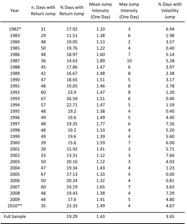
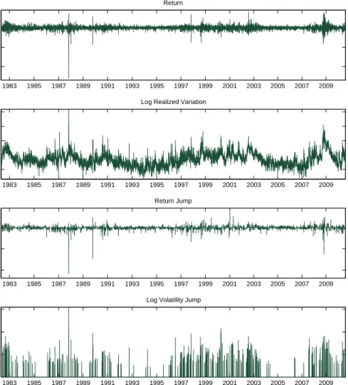
[Figure 1 about here.]

Figure 1 represents the time series of returns, log realized variation and jumps in return and volatil-ity. The highest levels of realized volatility were reached on “black Monday”, October 19, 1987, and the following day October 20, where returns were respectively about -26% and -9.6%. The test (7) detects jumps during both days. However for October 19, 1987, the intraday price changes were less drastic than on the following day, resulting in a lower jump variation. In October 20, 1987, jump variation was at the highest level. During that day negative jumps were combined with positive jumps, while on October 19, sequences of negative intraday returns dominated. The jumps test are carried out through the analysis withα=0.01 significance level.

Jumps in volatility are also identified for both October 19 and 20, 1987, with the volatility jump for October 19 being at the highest level. Accordingly, the market crash of October 19, 1987 is explained with jumps in returns and even more with a jump in volatility. This underscores the importance of allowing for volatility jumps in order to fully capture the dynamics of extreme events. Return jumps alone, identified with the testing methodology, are not able to fully account for extreme market events. Summary statistics for the intensity of jumps in return and in volatility are reported in Table 1.

[Table 1 about here.]

On average, there is less than one return jump per day. With significance levelα =0.01 and five

minutes sampling, the number of days with at least one intraday jump represents 19.29% of the sample period. The intraday jump intensity ranges from 0 to 10 jumps (maximum corresponding to October 19, 1987). Conditional on the presence of jumps there are on average 1.43 intraday return jumps each day. Regarding jumps in volatility, we find an intensity of about 6.65% of the trading days. The analysis for volatility jumps is also carried out at significance levelα=0.01 in eq. (24). As with jumps in return,

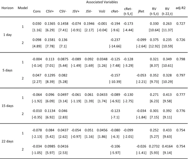
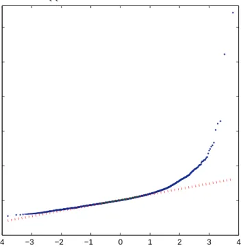
other significance levels are experimented. The chosen cutoff levelα =0.01 is empirically motivated

by the Quantile-Quantile Plot showed in Figure 2.

The empirical distribution with this cutoff level best approximates that of a standard normal distri-bution. Without a threshold, the residuals from the auxiliary GARCH model fitting deviate substantially from the assumed standard normal distribution. Only large departures from the standard normal distri-bution are categorized as volatility jumps.

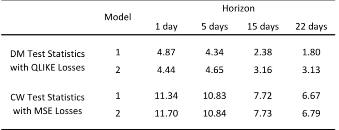
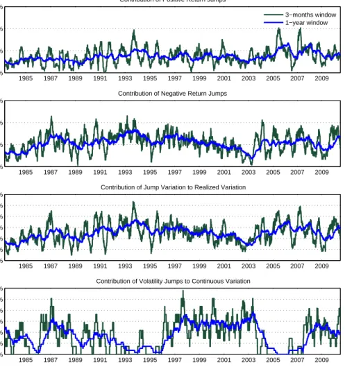
The contribution of return jumps to total return levels, the relative contribution of jump variation to the total variation and the contribution of volatility jumps to the continuous volatility are reported in Figure 3.

[Figure 3 about here.]

The contribution of negative jumps to negative returns appears to be higher, on average, than the contribution of positive jumps to the corresponding signed return. This jump sign asymmetry may account for the negative skewness observed in financial markets. Based on rolling averages of 3 months and 1 year windows, the contribution of the negative jumps to corresponding signed returns ranges from approximately 0.1% to 4.5%, on 3 months basis, and from 1% to 3.5%, on a yearly basis, while that of positive jumps ranges from 1% to 2.5%, on a yearly basis. Jump variation accounts for approximately 3% to 7% on a yearly basis. This statistic is in line with the ones reported by the previous literature despite the use of a different methodology to test for the presence of jumps. Corsi and Renò (2010), for example, report an average percentage over almost 28 years of about 6% for the S&P500 index, and Andersen et al. (2010) report an average percentage over five years that ranges from 2.1% to 5.8% for different stocks. By contrast, volatility jumps make a minor contribution to the continuous variation as they are more sporadic than return jumps. They account for about 0% to 8% of the continuous variation on a yearly basis, and for the entire sample period from 1982 to 2010 they represent 3.4% of continuous variation.

3.2 Forecasting with Jumps, Leverage effect, and Volatility Persistency

Given the measures of volatility and jump magnitude introduced previously, it is of interest to study their additional forecasting power for future volatility. The models proposed are based on the Heterogeneous Autoregressive (HAR) framework of Corsi (2009) and extend it by considering semivariances, jumps in return and in volatility, and the leverage effect due to continuous return and return jumps.

The realized volatility features long memory. The HAR model, although it does not belong formally to the class of long-memory models, represents a parsimonious approximation, which is able to closely

mimic such a stylized fact. In more detail, the benchmark model is

log(RV)_t,t+h=α+φd·log(RV)t+φ w

log(RV)_t−5,t+φmlog(RV)t−22,t+errort, (26)

where log(RV)_t,t+h is the average log realized variation between time t and t+h. The variables log(RV)_t−5,t = 1₅∑ti=t−4log(RVi) and log(RV)t−22,t = 221 ∑

t

i=t−21log(RVi) capture long memory

fea-tures of the volatility process. The coefficients of the model may be interpreted as the reaction of heterogeneous agents who forecast with different time horizons: daily, weekly and monthly. The rep-resentation of the HAR forecasting model based on realized variation instead of log realized variation,

RVt,t+h=α+φdRVt+φwRV(t−5,t]+φ(mt−22,t]+errort, (27)

is also considered. However, the last produces inferior forecasts and therefore results are summarized and discussed for the log-log model.

Several model extensions based on the HAR framework have been proposed in the recent literature: see, among others, Andersen et al. (2007a), Corsi and Renò (2010), and Patton and Sheppard (2011). Andersen et al. (2007a) included jump variation in forecasting volatility dynamics. Corsi and Renò (2010) studied the impact of the leverage effect on volatility by including past signed returns. Finally, Patton and Sheppard (2011) and Chen and Ghysels (2010) considered the use of realized semivariances to forecast volatility. None of the previous studies, however, used the return jumps themselves and jumps in volatility to generalize the HAR model.

Jumps in return arguably have an impact on future volatility. Contrary to the effect of jump vari-ations, this is interpreted as a leverage effect, which can manifest itself differently whether it comes about through continuous returns or jumps. In fact, although both components together generate the final leverage effect, their dynamics differ, as jumps have a very short impact on future volatility while continuous returns tend to have a persistent impact on future volatility.

Disentangling jump variation and continuous variation systematically improves volatility forecasts, and disentangling downside semivariation and upside semivariation also improves forecasts. We com-bine the ideas of Andersen et al. (2007a) and Patton and Sheppard (2011) by considering a complete decomposition into signed continuous and jump variation and this leads to even better forecasts. Nega-tive jump semivariation has in fact a completely different impact on future volatility than posiNega-tive jump semivariation. Lastly, jumps in volatility may also improve future volatility forecasts through the effect

of volatility trading strategies. Taking into account all these effects, the candidate model we propose is

log(RV)_t,t+h = α+β+·log CSV+_t+β−·log CSV−_t+γ+·log 1+JSV+_t+γ−·log 1+JSV−_t + θ·log(1+VolJ)_t+δ·cRet_t−+δw·cRet(−t−5,t]

+ ϑw·log(RV)(t−5,t]+ϑm·log(RV)(t−22,t]+errort, (28)

where past negative returns and jumps are defined by cRet_t− =1{cRett<0}·cRett, and cRet

− (t−5,t] =

1

5∑

t

i=t−4·cReti−. Note that the realized jump semivariances already capture the effect of return jumps,

since they are derived from them. The interpretation of their effects is that of jump risks that capture jump leverage effects. Therefore, return jumps are not included in this model specification.

Given that one of the goals of this study is volatility forecasting, one can argue that such a model may be overparameterized and therefore may lead to poor out-of-sample results. As we will show in the next sections this is not (entirely) the case. Nevertheless, to overcome this problem we consider a simplified version of model (28) that differs from the previous one by discarding jump semivariations, the weekly persistency in the leverage effect, and the jumps in volatility3. Moreover the impact of jump semivariations on future volatility are being replaced by that of return jumps which is to be interpreted as a leverage effect due to jumps:

log(RV)_t,t+h = α+β+·log CSV+_t+β−·log CSV−_t

+ δ·cRet_t−+ϕ·jRett+ϑw·log(RV)(t−5,t]+ϑm·log(RV)(t−22,t]+errort. (29)

This model is very simple, consisting only of seven parameters to be estimated, e.g., three parameters less than the LHAR-CJ model proposed by Corsi and Renò (2010). Still, the model focuses on the most relevant effects for volatility forecasting: downside risk, leverage effect, and the HAR structure capturing long-memory.

The models are estimated by OLS with Newey and West (1987) covariance matrix correction to account for serial correlation. The bandwidth used is 2(h−1), wherehis the forecasting horizon.

3_{We tried to discard these effects one-by-one with an approach similar to backward stepwise subset selection and verified}

4

Empirical Evidence

4.1 Leverage Effect, Volatility Feedback Effect, and Persistency

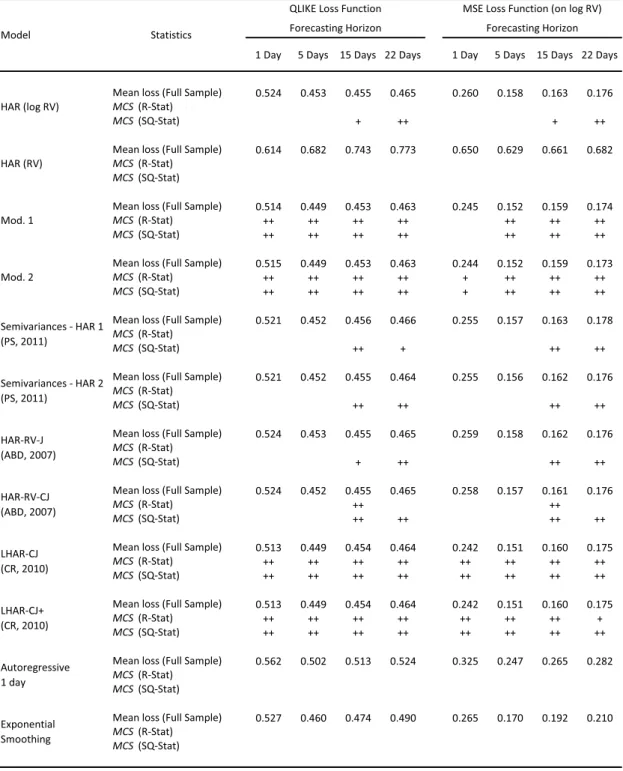
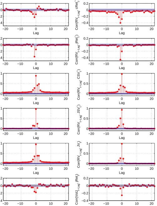
Leverage and volatility feedback effects are commonly studied by mean of correlations. Bollerslev et al. (2006) provide exhaustive evidence of the leverage effect at high-frequency by studying cross-correlations among return and volatility series for a horizon spanning several days. Exploiting the methodology we use to disentangle the continuous and jump components of return and volatility dy-namics, we present new evidence of leverage and volatility feedback effects arising from both contin-uous and jump components. Moreover, we use signed intraday returns to capture sign asymmetries. Figure 4 reports cross-correlations among different components of the return and quadratic variation as evidence of leverage and volatility feedback effects, and persistency in volatility.

[Figure 4 about here.]

As in Bollerslev et al. (2006), the leverage effect (negative correlation between RVt+h and Rett)

is significant for prolonged days, while there is no evidence of volatility feedback effect (negative correlation betweenRVt−h andRett). The sign and size asymmetry of the leverage effect becomes

evident as negative returns generate all the negative correlation of return and lagged volatility (see top right plot, figure 4) and the magnitude of this effect is higher than the positive correlation between positive returns and realized variation. Regarding volatility feedback effect, we observe a negative correlation between realized variation and future negative returns. However, this correlation is rather small and insufficient to generate the negative size asymmetry, as realized variation has an even higher magnitude of correlation with positive future returns.

Jumps in return are highly responsible for the leverage effect. The negative correlation between jumps and future volatility is very high in magnitude (see second row of figure 4) but this effect is short lived, lasting only one day period. The plots on the third and fourth rows of figure 4 reports the cross correlation of realized variation with signed continuous and jump semivariations. All those components have an impact on future volatility and they represent different sources of risk.

The persistence in volatility is also examined. It is well known that volatility is autocorrelated for a prolonged period of time. Evidence is found in Ding et al. (1993) for the S&P500 stock index. Models to capture the persistence in conditional volatility have been proposed in their early stage by Engle and Bollerslev (1986) and Baillie et al. (1996). This autocorrelation is one of the drivers of the volatility

feedback effect. As mentioned above, when an increase in volatility is associated with an expectation of higher future volatility, market participants may discount this information, resulting in an immediate drop in stock prices. We find that the persistence in volatility is generated by the continuous component of the return variation. Clearly, jump variation has a confounding effect on realized variation as well, but this effect is also short lived (The cross-correlations of realized variation with continuous variation and with jump variation are reported in the fifth row of figure 4.)

Finally, both continuous return and jumps in return are negatively and contemporaneously corre-lated with volatility jumps. Moreover, they have a small and short-lived impact on future volatility jumps. On the other hand, volatility jumps also have a short-lived impact only on future return jumps and continuous returns (Cross-correlations of continuous returns and return jumps with jumps in volatil-ity, depicting asymmetries for the jump components of the volatilvolatil-ity, are represented in the last row of Figure 4).

4.2 In-Sample Analysis

Estimation results of the proposed forecasting models are discussed in this section. The in-sample evaluations are based on different horizons. The regression results of the candidate models are reported in Table 2, for horizons of 1, 5, 15 and 22 days.

[Table 2 about here.]

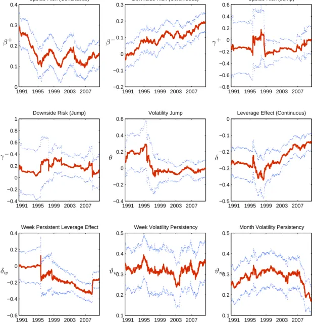
In order to check the stability of the coefficients, regressions are run for different overlapping sub-samples. As the full sample period is relatively long, consisting of more than 28 years, it is likely that structural breaks have occurred. This seems to be the case, as some coefficients estimated by includ-ing data for the initial 8 years, from 1982 to 1989 (the forecasts are relative to the period 1990-1997), appear to differ slightly from those estimated by using data starting from 1990. Conversely, the coeffi-cients associated with the model for the last 20 years are relatively stable. Figure 5 reports the estimated coefficients of one period forecast of model (28) with rolling subsamples of 2000 observations (corre-sponding to almost 8 years).

[Figure 5 about here.]

With an in-deep inspection, the difference of the coefficient estimates for the initial subsample from those of the remaining subsample is mainly caused by the market crash of October 1987. The sample

period is therefore reduced and the results of the in-sample analysis contained in table 2 are relative to the subperiod from January 4, 1988 to August 6, 20104. By contrast, the out-of-sample evaluations of the next sections, as they are performed using rolling forecasts, will be based on the whole sample period. Volatility jumps have a marginal power to forecast the one period ahead volatility only with the initial subsamples, which contain the market crash data, while for the remaining subsamples they do not add further value. This indicates that volatility jumps are useful for forecasting during extremely agitated periods.

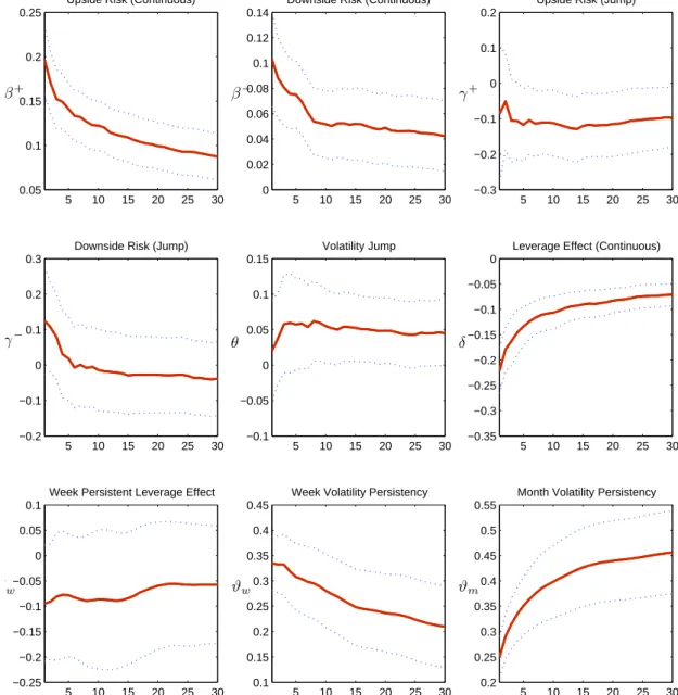
To check the stability of the estimates for different forecasting horizons, figure 6 reports the esti-mated coefficients for forecasting horizons ranging from 1 day to 30 days. The estiesti-mated parameters appear to be well-behaved. The 95% forecast confidence intervals (adjusted with Newey-West serial correlation consistent standard errors), are relatively large for the coefficients associated with jump semivariations.

[Figure 6 about here.]

The following results from the estimation are worth remarking on. “Bad volatilities” have a sig-nificant impact on future volatility. Both continuous and jump downside semivariations increase future realized variation. However, when “good volatilities” are disentangled into upside continuous variation and upside jump variation, a striking difference emerges. The effect of upside continuous semivariation on future volatility is still positive and statistically significant, but that of the upside jump semivaria-tion is on average negative and negligible. This may well answer the critique advanced by Corsi et al. (2010) as they argue that influential studies such as Andersen et al. (2007a) and Forsberg and Ghysels (2007), among others, find a negative or null impact of jumps (more appropriately jump variation) on future volatility, while economic theory suggests the opposite. In fact, one needs to distinguish between downside and upside jumps. Future volatility is indeed increasing with downside jump variation as jump variations are likely associated with an increase in uncertainty on fundamental values. However the effect of upside jump variation does not necessarily increase future volatility. This would be con-sistent with the economic model of Veronesi (1999). Intuitively, a positive jump is associated with the occurrence of good news as well as the expectation of higher future returns. The effect of the latter is able to offset the effect of an increasing uncertainty. The future volatility given the occurrence of a

4_{Although the estimated coefficients obtained by using the full sample data, including the market crash of 1987, do not}

differ substantially from the ones reported in table 2, there may be a minor loss in term of consistency of the estimates by using the full sample data. However, the signs associated with all significant coefficients are the same for the various subsamples.

positive jump is therefore lower than the one associated with the occurrence of a negative jump. Consistent with the leverage effect, both continuous and jump components of the return have a significant impact on future volatility. As mentioned previously, the persistency in leverage effect is captured mainly by the continuous component. In fact, as the forecasting horizon increases, the leverage effect generated by past jumps becomes less statistically significant. On the contrary, the coefficient associated with the negative continuous return over the past day and over the past week remains statistically significant even for longer forecasting horizons.

Concerning long memory features, the persistence parameter associated with the one week and one month realized volatility is highly statistically significant for all horizons. Ultimately, jumps in volatility (continuous variation) do not appear to be statistically significant. Given that volatility jumps are present during extremely agitated periods, their null forecasting performance on the short horizon is due to the fact that only a few volatility jumps are identified for the sample period under investigation. There are in fact volatility jumps for only 3.6% of the sample days.

Finally, by examining the (in-sample) performance of the simplified model (29) in comparison with the one of the full model, the losses in accuracy that occur for the simplified model are negligible based on the adjustedR2.

4.3 Out-of-Sample Forecasting Performance

The methodology used to assess the forecasting performance of the proposed models is presented in this section. The analysis is based on the out-of-sample predictive accuracy of these models in comparison to the HAR-RV model (26). The predicted variable is the cumulative average log realized variation between timet andt+h. For predictions of horizonsh>1, a “direct method” is employed, that is, the model specifies only the relation between log(RV)_t,t+hand the regressors at timet. The evaluation of the performance is done recursively with rolling windows. The forecasting horizons considered are

h={1,5,15,22}.

The recursive procedure is applied as follows: The forecasts are generated by using an in-sample estimation window of 2000 observations, corresponding to about eight years, starting from April 28, 1982. Forh=1, the performance is evaluated on 5040 out-of-sample data points, corresponding to about 20 years. The forecasting performance is based on the MSE function of the log realized variation forecasts and the negative QLIKE loss function:

MSE=_ln(RV\₎ t,t+h|_Ft−ln(RV)t,t+h 2 , (30) QLIKE=_ln(RV\)_t,t+h|F t+ RVt,t+h \ RVt,t+h|_Ft . (31)

The MSE is a symmetric loss function while QLIKE is asymmetric. Patton (2011) shows that the QLIKE loss function is robust to noise in the volatility proxy, as volatility forecasts represent a case where the true values are not observable. Moreover, this function has certain optimal properties in that it is less sensitive to large observations by more heavily penalizing under-predictions then over-predictions. It is therefore more suited to yield model rankings in the presence of imperfect proxies.

To test for the superior forecasting performance of the proposed models over the benchmark HAR-RV model, the Diebold and Mariano (1995) test is employed. The asymptotic variance of the loss differential (of each model and the HAR-RV model) is estimated with Newey-West HAC consistent sample variance as suggested by Giacomini and White (2006). Clark and McCracken (2001) show that in the presence of nested models, the distribution of the Diebold-Mariano test statistics for mean square error losses, under the null, can be nonstandard. Therefore the test of forecasting performance for mean square error losses is based on the Clark and West (2007) test statistic, which appropriately corrects the loss differential. Table 3 reports the test statistics under the null of equal forecasting performance for each model pair. A positive loss differential represents a superior average forecasting performance of the proposed model with respect to the HAR-RV.

[Table 3 about here.]

At the 99% confidence level, the proposed models outperform the base model for forecasting hori-zons of one day and five days. For longer forecasting horihori-zons, overall the models also perform well, with the reduced model (eq. 29) achieving surprisingly high performance. Based on the QLIKE loss function, the outperformance of the full model (28) compared with the HAR-RV model is only weakly statistically significant. This is a warning signal that model (28) is probably overparameterized, al-though as shown in the next section, outperforming the benchmark HAR-RV model in forecasting long-run volatility seems to be a difficult task.

4.4 Model Confidence Set

The HAR-RV model in logarithmic form generally has a good out-of-sample forecasting performance. In an attempt to raise the bar, other reference models recently proposed in the literature are considered. First, we test the performance of the HAR model for the realized variation, which yielded the lowest forecasting power among all the candidate models when evaluated on the loss functions (30) and (31). Thus, results for that model are not reported. Then, we investigate the accuracy of the volatility forecasts for several models involving two model specifications of Andersen et al. (2007a), named HAR-RV-J and HAR-RV-CJ (eq. 13, p. 709, and eq. 28, p. 715), which explicitly take into account continuous and jump variation; two models proposed by Patton and Sheppard (2011) based on semivariances, one with complete decomposition into semivariances and the other with a downside semivariance only for the daily component (eq. 19, p. 16, and eq. 17, p. 13, without upside semivariance); and two models of Corsi and Renò (2010) that add the leverage effect, named LHAR-CJ and LHAR-CJ+ (eq. 2.4, p. 8, and table 3, p. 16). Finally, simple and commonly used models are also taken into account. These are an autoregressive model on the daily component only and an exponential smoothing model on log realized variation. The last is popularly used by risk practitioners (see Taylor, 2004) and is specified as

\

log(RV)_t,t+h=α·log(RV)_t−h,t+ (1−α)·log(\RV)_t−h,t (32)

with parameterα optimized for each rolling window following

arg min α

∑

All the models, except the HAR-RV, are evaluated on log realized variation. They are also estimated on the same rolling window and evaluated on the same out-of-sample data points. It is also worth men-tioning that jumps detection and jump variation estimation are executed in the same way as described in this paper.5

In order to evaluate forecasts of those models, the model confidence set (MCS) methodology of Hansen et al. (2003, 2011) is the most well-suited. The comparison is done among a set of models, as pairwise comparisons would not be appropriate. The methodology allows the models to be ranked based

5_{In their original work, Andersen et al. (2007a) do not apply a test for significant jump detection but jumps are identified}

as positive differences betweenRV andBV. Corsi and Renò (2010) apply a test based on the difference betweenRVand a threshold estimator for the continuous variation. Numerically, the results may differ slightly with different jump identification procedures. However, the performance of our proposed models is robust even compared to other testing procedures for jumps.

on a given loss function and it gives indication of whether the forecast performances are significantly different. Out of the surviving models in the confidence set, the interpretation is that they have equal predictive ability and they yield the best forecasts given a confidence level.

The model confidence set approach allows the user to specify different criteria to establish equal forecasting performance for the model set and subsets. We use both the “range” statistic, and the “semi-quadratic” statistic: TR = max i,j∈Mset d¯i j q c var d¯i j , (33) TSQ =

∑

where ¯di jis the mean loss differential between each pair combination of models.

Table 4 reports the model confidence set and the selected models at the 5% and 15% significance levels. The model confidence set p-value is obtained through a block bootstrap procedure. An autore-gressive process is estimated for eachdi j, the loss differential between each modeliand j, and the lag

length for it is determined by Akaike information criteria as suggested by Hansen et al. (2003). The block length for the bootstrap procedure is then fixed as the maximum lag length amongdi jand it varies

between 9 and 30 depending on the forecasting horizon and the loss function used. 5000 bootstrap rep-etitions are used to compute the test statistics. The model confidence set p-value obtained by using the semi-quadratic test statistics is less conservative then the one obtained by using the range statistics. The surviving model set after using the semi-quadratic test statistic is therefore larger than the set obtained by using the range test statistic.

[Table 4 about here.]

Overall, the best forecasting models for all different horizons are the candidate models (28) and (29) and the two LHAR-CJ models proposed by Corsi and Renò (2010), which take into account past negative return without disentangling return jumps size. The reduced model of eq. (29) achieved equal forecasting performance, compared with the LHAR-CJ+ model, with a lower model complexity (4 variables less). Jumps in return indeed substantially improve the forecasting performance, while jumps in continuous variation (called volatility jumps) are infrequent and have a minor effect on future realized

variation. Jumps in quadratic variation are in fact mainly due to return jumps. For the one period ahead forecast, the full model (28), which includes volatility jumps, does not survive based on the MSE loss function. However, it does survive based on the QLIKE loss function. This is due to the fact that by adding volatility jumps, the model tends to produce marginally less conservative forecasts of volatility. The QLIKE loss, since it less heavily penalizes over-predictions then under-predictions, still selects this model. Not surprisingly, the best forecasting models are the ones that include the leverage effect.

Finally, the following considerations can be pointed out for the simplest models: For long horizons, the simple HAR-RV model is hard to beat. As has already been shown previously in the literature, the autoregressive model that takes only the daily component into account is not selected for any fore-casting horizon and loss function used, pointing to the importance of correctly modeling long-memory. Moreover, the exponential smoothing model, often used in practice, is clearly outperformed.

5

Conclusion

This paper analyzed the performance of volatility forecasting models that take into account downside risk, jumps, and the leverage effect. The volatility forecasting model proposed consists of the following ingredients: First, the size of return jumps is identified based on the test of Lee and Mykland (2008). Second, jump variation and continuous variation are disentangled based on the methodology proposed by Andersen et al. (2010). Third, the size of jumps in volatility is also identified with inference based on an auxiliary AR-GARCH model. Finally, signed jump and continuous semivariations are computed using signed intraday returns. The best candidate model for forecasting realized volatilities must simul-taneously take into account return jumps, “good” and “bad” risks, leverage effect, and strong volatility persistence (i.e. long memory).

The model is motivated by overwhelming evidence of asymmetries in financial time series. We show that correlation asymmetries are present for both continuous and jump components among return and volatility processes. Moreover, asymmetries exist not only in size but also in sign, justifying the use of semivariances in forecasting volatility.

The forecasting model is very simple to implement as based on the parsimonious HAR framework. The gain over the base HAR-RV in terms of out-of-sample forecasting power is substantial and this is especially true for short and mid forecasting horizons. Therefore, volatility forecasts with return and jump asymmetries are warranted.

References

Andersen T, Bollerslev T, Diebold F. 2007a. Roughing it up: Including jump components in the mea-surement, modeling and forecasting of return volatility. Review of Economics and Statistics 89: 701–720.

Andersen T, Bollerslev T, Diebold F, Ebens H. 2001a. The distribution of realized stock return volatility.

Journal of Financial Economics61: 43–76.

Andersen T, Bollerslev T, Diebold F, Labys P. 2001b. The distribution of realized exchange rate

volatil-ity. Journal of the American Statistical Association96: 42–55.

Andersen T, Bollerslev T, Diebold F, Labys P. 2003. Modeling and forecasting realized volatility.

Econometrica71: 579–625.

Andersen T, Bollerslev T, Dobrev D. 2007b. No-arbitrage semi-martingale restrictions for continuous-time volatility models subject to leverage effects, jumps and iid noise: Theory and testable distribu-tional implications. Journal of Econometrics138: 125–180.

Andersen T, Bollerslev T, Frederiksen P, Ørregaard Nielsen M. 2010. Continuous-time models, real-ized volatilities, and testable distributional implications for daily stock returns. Journal of Applied

Econometrics25: 233–261.

Bae J, Kim C, Nelson C. 2007. Why are stock returns and volatility negatively correlated? Journal of

Empirical Finance14: 41–58.

Baillie R, Bollerslev T, Mikkelsen H. 1996. Fractionally integrated generalized autoregressive condi-tional heteroskedasticity. Journal of Econometrics74: 3–30.

Bandi F, Reno R. 2010. Time-varying leverage effects.Journal of EconometricsForthcoming. Barndorff-Nielsen O, Kinnebrock S, Shephard N. 2010. Measuring downside risk - realized

semivari-ance. In Bollerslev T, Russel J, Watson M (eds.)Volatility and Time Series Econometrics, chapter 7. Oxford University Press, 117–137.

Barndorff-Nielsen O, Shephard N. 2002. Econometric analysis of realized volatility and its use in estimating stochastic volatility models. Journal of the Royal Statistical Society, Series B64: 253– 280.

Barndorff-Nielsen O, Shephard N. 2004. Power and bipower variation with stochastic volatility and jumps. Journal of Financial Econometrics2: 1–37.

Barndorff-Nielsen O, Shephard N. 2006. Econometrics of testing for jumps in financial economics using bipower variation.Journal of Financial Econometrics4: 1–30.

Bekaert G, Wu G. 2000. Asymmetric volatility and risk in equity markets.Review of Financial Studies

Bollerslev T, Kretschmer U, Pigorsch C, Tauchen G. 2009. A discrete-time model for daily s&p500 returns and realized variations: Jumps and leverage effects.Journal of Econometrics150: 151–166. Bollerslev T, Litvinova J, Tauchen G. 2006. Leverage and volatility feedback effects in high-frequency

data. Journal of Financial Econometrics4: 353.

Broadie M, Chernov M, Johannes M. 2007. Model specification and risk premia: Evidence from futures options. Journal of Finance62: 1453–1490.

Campbell J, Hentschel L. 1992. No news is good news: An asymmetric model of changing volatility in stock returns. Journal of Financial Economics31: 281–318.

Chen X, Ghysels E. 2010. News - good or bad - and its impact on volatility predictions over multiple horizons. Review of Financial Studies24: 46–81.

Chernov M, Gallant A, Ghysels E, Tauchen G. 2003. Alternative models for stock price dynamics.

Journal of Econometrics116: 225–257.

Christie A. 1982. The stochastic behavior of common stock variances: Value, leverage and interest rate effects. Journal of Financial Economics10: 407–432.

Clark T, McCracken M. 2001. Tests of equal forecast accuracy and encompassing for nested models.

Journal of Econometrics105: 85–110.

Clark T, West K. 2007. Approximately normal tests for equal predictive accuracy in nested models.

Journal of Econometrics138: 291–311.

Corsi F. 2009. A simple approximate long-memory model of realized volatility. Journal of Financial

Econometrics7: 174–196.

Corsi F, Pirino D, Renò R. 2010. Threshold bipower variation and the impact of jumps on volatility forecasting. Journal of Econometrics159: 276–288.

Corsi F, Renò R. 2010. Discrete-time volatility forecasting with persistent leverage effect and the link with continuous-time volatility modeling. Working Paper.

Diebold F, Mariano R. 1995. Comparing predictive accuracy.Journal of Business & Economic Statistics

13: 253–263.

Ding Z, Granger C, Engle R. 1993. A long memory property of stock market returns and a new model.

Journal of Empirical Finance1: 83–106.

Duffie D, Pan J, Singleton K. 2000. Transform analysis and asset pricing for affine jump-diffusions.

Econometrica68: 1343–1376.

Engle R, Bollerslev T. 1986. Modelling the persistence of conditional variances. Econometric Reviews

Eraker B. 2004. Do stock prices and volatility jump? reconciling evidence from spot and option prices.

Journal of Finance59: 1367–1404.

Eraker B, Johannes M, Polson N. 2003. The impact of jumps in volatility and returns. Journal of

Finance58: 1269–1300.

Forsberg L, Ghysels E. 2007. Why do absolute returns predict volatility so well? Journal of Financial

Econometrics5: 31–67. ISSN 1479-8409.

French K, Schwert G, Stambaugh R. 1987. Expected stock returns and volatility. Journal of Financial

Economics19: 3–29.

Giacomini R, White H. 2006. Tests of conditional predictive ability.Econometrica74: 1545–1578. Hansen P, Lunde A. 2006a. Consistent ranking of volatility models. Journal of Econometrics131:

97–121.

Hansen P, Lunde A. 2006b. Realized variance and market microstructure noise. Journal of Business

and Economic Statistics24: 127–161.

Hansen P, Lunde A, Nason J. 2003. Choosing the best volatility models: The model confidence set approach. Oxford Bulletin of Economics and Statistics65: 839–861.

Hansen P, Lunde A, Nason J. 2011. The model confidence set. Econometrica79: 453–497.

Lee S, Mykland P. 2008. Jumps in financial markets: A new nonparametric test and jump dynamics.

Review of Financial studies21: 2535–2563.

Mykland P, Zhang L. 2009. Inference for continuous semimartingales observed at high frequency.

Econometrica77: 1403–1445.

Newey W, West K. 1987. A simple, positive semi-definite, heteroskedasticity and autocorrelation con-sistent covariance matrix. Econometrica55: 703–708.

Patton A. 2011. Volatility forecast comparison using imperfect volatility proxies. Journal of

Econo-metrics160: 246–256.

Patton A, Sheppard K. 2011. Good volatility, bad volatility: Signed jumps and the persistence of volatility. Working Paper.

Schwert G. 1989. Why does stock market volatility change over time? Journal of Finance44: 1115. Taylor J. 2004. Volatility forecasting with smooth transition exponential smoothing. International

Journal of Forecasting20: 273–286.

Todorov V, Tauchen G. 2010. Volatility jumps. Forthcoming in Journal of Business and Economic

Veronesi P. 1999. Stock market overreaction to bad news in good times: A rational expectations equi-librium model. Review of Financial Studies12: 975–1007.

zĞĂƌ Ŷ͘ĂLJƐǁŝƚŚ ZĞƚƵƌŶ:ƵŵƉ йĂLJƐǁŝƚŚ ZĞƚƵƌŶ:ƵŵƉ DĞĂŶ:ƵŵƉ /ŶƚĞŶƐŝƚLJ ;KŶĞĂLJͿ DĂdž:ƵŵƉ /ŶƚĞŶƐŝƚLJ ;KŶĞĂLJͿ йĂLJƐǁŝƚŚ sŽůĂƚŝůŝƚLJ :ƵŵƉ ϭϵϴϮΎ ϯϭ ϭϳ͘ϵϮ ϭ͘ϭϬ ϯ ϲ͘ϵϰ ϭϵϴϯ Ϯϵ ϭϭ͘ϱϭ ϭ͘ϯϴ ϲ ϭ͘ϵϴ ϭϵϴϰ ϰϴ ϭϵ͘Ϭϱ ϭ͘ϭϯ Ϯ ϯ͘ϱϳ ϭϵϴϱ ϱϬ ϭϵ͘ϳϲ ϭ͘ϮϮ ϰ Ϭ͘ϰϬ ϭϵϴϲ ϰϴ ϭϴ͘ϵϳ ϭ͘ϲϬ ϳ ϱ͘ϭϰ ϭϵϴϳ ϯϲ ϭϰ͘ϲϯ ϭ͘ϴϵ ϭϬ ϱ͘Ϯϴ ϭϵϴϴ ϰϱ ϭϳ͘ϴϲ ϭ͘ϰϳ ϲ ϯ͘ϵϳ ϭϵϴϵ ϰϮ ϭϲ͘ϲϳ ϭ͘ϰϴ ϴ Ϯ͘ϯϴ ϭϵϵϬ ϰϳ ϭϴ͘ϲϱ ϭ͘ϱϭ ϱ ϯ͘ϭϳ ϭϵϵϭ ϰϴ ϭϵ͘Ϭϱ ϭ͘ϰϲ ϴ Ϯ͘ϳϴ ϭϵϵϮ ϲϬ Ϯϯ͘ϵ ϭ͘ϰϳ ϴ ϭ͘ϮϬ ϭϵϵϯ ϲϳ Ϯϲ͘ϱϵ ϭ͘ϱϭ ϲ Ϭ͘ϰϬ ϭϵϵϰ ϱϳ ϮϮ͘ϳϭ ϭ͘ϰϳ ϱ ϭ͘ϱϵ ϭϵϵϱ ϰϴ ϭϵ͘Ϯ ϭ͘ϯϴ ϰ Ϭ͘ϰϬ ϭϵϵϲ ϰϵ ϭϵ͘ϲ ϭ͘ϰϵ ϱ ϰ͘ϰϬ ϭϵϵϳ ϰϴ ϭϵ͘ϯϱ ϭ͘ϳϳ ϲ ϳ͘Ϯϲ ϭϵϵϴ ϰϴ ϭϵ͘Ϯ ϭ͘ϯϯ ϰ ϱ͘ϮϬ ϭϵϵϵ ϰϵ ϭϵ͘ϲ ϭ͘ϯϵ ϰ ϱ͘ϲϬ ϮϬϬϬ ϯϵ ϭϱ͘ϲ ϭ͘ϱϵ ϳ ϲ͘ϬϬ ϮϬϬϭ ϯϵ ϭϱ͘ϵϮ ϭ͘ϰϭ ϯ ϱ͘ϳϭ ϮϬϬϮ ϯϯ ϭϯ͘ϯϭ ϭ͘ϭϮ ϯ ϳ͘ϲϲ ϮϬϬϯ ϱϬ ϮϬ͘ϭϲ ϭ͘ϭϮ ϯ ϰ͘Ϭϯ ϮϬϬϰ ϰϳ ϭϵ͘ϯϰ ϭ͘ϰϯ ϰ ϭ͘Ϯϯ ϮϬϬϱ ϲϳ Ϯϳ͘ϭϯ ϭ͘ϯϯ ϰ Ϭ͘ϬϬ ϮϬϬϲ ϱϬ ϮϬ͘Ϯϰ ϭ͘ϯϮ ϰ Ϭ͘ϴϭ ϮϬϬϳ ϲϬ Ϯϰ͘ϭϵ ϭ͘ϲϱ ϳ ϯ͘ϲϯ ϮϬϬϴ ϰϴ ϭϵ͘ϰϯ ϭ͘ϯϴ ϰ ϳ͘Ϯϵ ϮϬϬϵ ϰϰ ϭϳ͘ϲ ϭ͘ϰϭ ϱ ϰ͘ϴϬ ϮϬϭϬΎΎ ϯϱ Ϯϯ͘ϯϯ ϭ͘ϰϵ ϰ ϰ͘ϲϳ &Ƶůů^ĂŵƉůĞ ϭϵ͘Ϯϵ ϭ͘ϰϯ ϯ͘ϲϱ

Table 1: Jump Descriptive Statistics

NOTE: The table reports the number or days with return jumps, their percentage, the average daily jump intensity conditional on the presence of at least one jump, the maximum daily jump intensity, and the percentage of days with jumps in continuous variation. All the statistics are sorted by year. The tests for jumps in return and in continuous variation are conducted with significance levelα=0.01. * The sample period for 1982 starts on April, 28. ** The sample period for 2010 stops on August,

ŽŶƐ ^sн ^sͲ :^sн :^sͲ sŽů: ĐZĞƚͲ ĐZĞƚͲ ;ƚͲϱ͕ƚ΁ ũZĞƚ Zs ;ƚͲϱ͕ƚͿ Zs ;ƚͲϮϮ͕ƚͿ Ϭ͘ϬϯϬ Ϭ͘ϭϯϲϱ Ϭ͘ϭϰϱϴ ͲϬ͘Ϭϳϰ Ϭ͘ϭϵϰϲ ͲϬ͘ϬϬϭ ͲϬ͘ϭϵϰ ͲϬ͘ϭϳϯ Ϭ͘ϯϯϬ Ϭ͘Ϯϲϯ Ϭ͘ϳϮϳ ΀ϭ͘ϭϲ΁ ΀ϲ͘Ϯϵ΁ ΀ϳ͘ϰϭ΁ ΀ͲϬ͘ϵϭ΁ ΀Ϯ͘ϭϳ΁ ΀ͲϬ͘Ϭϰ΁ ΀Ͳϵ͘ϲ΁ ΀Ͳϰ͘ϰϰ΁ ΀ϭϬ͘ϲϰ΁ ΀ϭϭ͘ϯϳ΁ Ϭ͘Ϭϵϴ Ϭ͘ϭϱϴϭ Ϭ͘ϭϯϲ ͲϬ͘Ϯϯϳ ͲϬ͘Ϭϵϵ Ϭ͘ϯϳϱ Ϭ͘Ϯϯϱ Ϭ͘ϳϮϲ ΀ϰ͘ϴϵ΁ ΀ϳ͘ϳϴ΁ ΀ϳ͘ϭ΁ ΀Ͳϭϰ͘ϲϲ΁ ΀ͲϮ͘ϲϰ΁ ΀ϭϮ͘ϵϮ΁ ΀ϭϬ͘ϱϵ΁ ͲϬ͘ϬϬϰ Ϭ͘ϭϭϯ Ϭ͘Ϭϴϳϱ ͲϬ͘Ϭϴϵ Ϭ͘ϬϵϮ Ϭ͘Ϭϯϰϴ ͲϬ͘ϭϮϱ ͲϬ͘ϭϮϴ Ϭ͘ϯϮϭ Ϭ͘ϯϰϵ Ϭ͘ϳϵϴ ΀ͲϬ͘ϭϰ΁ ΀ϳ͘Ϭϭ΁ ΀ϱ͘ϰϰ΁ ΀Ͳϭ͘ϰϵ΁ ΀ϭ͘ϲϵ΁ ΀ϭ͘Ϯϲ΁ ΀Ͳϳ͘ϰϴ΁ ΀Ͳϯ͘Ϯϵ΁ ΀ϴ͘ϯϳ΁ ΀ϭϬ͘ϲϭ΁ Ϭ͘Ϭϰϳ Ϭ͘ϭϮϵϱ Ϭ͘ϬϴϮ ͲϬ͘ϭϱϳ ͲϬ͘Ϭϱϯ Ϭ͘ϯϱϮ Ϭ͘ϯϮϴ Ϭ͘ϳϵϳ ΀Ϯ͘Ϯϳ΁ ΀ϴ͘ϯϵ΁ ΀ϱ͘Ϯϴ΁ ΀ͲϭϬ͘ϯϵ΁ ΀ͲϮ͘Ϯϭ΁ ΀ϵ͘ϳϯ΁ ΀ϭϬ͘Ϯϵ΁ ͲϬ͘Ϭϲϰ Ϭ͘Ϭϵϲ Ϭ͘Ϭϰϵϳ ͲϬ͘Ϭϲϭ Ϭ͘Ϭϲϭ Ϭ͘Ϭϰϯϯ ͲϬ͘Ϭϴϵ ͲϬ͘ϭϯϬ Ϭ͘Ϯϳϭ Ϭ͘ϰϭϯ Ϭ͘ϳϳϳ ΀Ͳϭ͘ϵϮ΁ ΀ϲ͘Ϭϵ΁ ΀ϯ͘ϭϰ΁ ΀Ͳϭ͘ϭϵ΁ ΀ϭ͘ϯϵ΁ ΀ϭ͘ϳϰ΁ ΀Ͳϲ͘ϵϮ΁ ΀ͲϮ͘ϳϱ΁ ΀ϲ͘Ϯϯ΁ ΀ϵ͘ϱϴ΁ ͲϬ͘ϬϭϬ Ϭ͘ϭϭϯϰ Ϭ͘Ϭϰϲ ͲϬ͘ϭϮϯ ͲϬ͘Ϭϯϰ Ϭ͘ϯϬϭ Ϭ͘ϯϵϮ Ϭ͘ϳϳϲ ΀ͲϬ͘ϯϱ΁ ΀ϲ͘ϵϮ΁ ΀Ϯ͘ϴϯ΁ ΀Ͳϳ͘ϭ΁ ΀Ͳϭ͘ϴϰ΁ ΀ϳ͘ϭϱ΁ ΀ϵ͘ϭϭ΁ ͲϬ͘Ϭϳϴ Ϭ͘Ϭϴϰ Ϭ͘Ϭϰϯϳ ͲϬ͘Ϭϱϰ Ϭ͘Ϭϱϭ Ϭ͘Ϭϰϱϲ ͲϬ͘ϬϴϬ ͲϬ͘Ϭϵϵ Ϭ͘ϮϱϮ Ϭ͘ϰϯϯ Ϭ͘ϳϱϰ ΀ͲϮ͘ϭϯ΁ ΀ϱ͘ϰϮ΁ ΀Ϯ͘ϲϮ΁ ΀ͲϬ͘ϵϳ΁ ΀ϭ͘ϭϲ΁ ΀ϭ͘ϴϲ΁ ΀Ͳϲ͘ϯ΁ ΀ͲϮ͘Ϭϭ΁ ΀ϱ͘Ϯϳ΁ ΀ϵ͘ϲϯ΁ ͲϬ͘Ϭϯϰ Ϭ͘Ϭϵϴϱ Ϭ͘Ϭϰϭϲ ͲϬ͘ϭϬϲ ͲϬ͘ϬϮϲ Ϭ͘ϮϳϯϮ Ϭ͘ϰϭϲϰ Ϭ͘ϳϱϰ ΀Ͳϭ͘Ϭϱ΁ ΀ϱ͘ϵϳ΁ ΀Ϯ͘ϱϯ΁ ΀Ͳϱ͘ϵϳ΁ ΀Ͳϭ͘ϰϭ΁ ΀ϱ͘ϵϯ΁ ΀ϵ͘ϭϰ΁ ϮϮĚĂLJƐ ϭ Ϯ ϱĚĂLJƐ ϭ Ϯ ϭϱĚĂLJƐ ϭ Ϯ ,ŽƌŝnjŽŶ DŽĚĞů ƐƐŽĐŝĂƚĞĚsĂƌŝĂďůĞƐ ĂĚũͲZϮ ϭĚĂLJ ϭ Ϯ

Table 2: In Sample Regressions

NOTE: The table contains estimates of the coefficients and t-statistics, in square brackets, based on Newey-West HAC consis-tent standard errors, for the two model specifications. Model 1 and model 2 correspond to equations (28) and (29), respectively. The models are estimated for forecasting horizons of 1, 5, 15 and 22 days.

ϭĚĂLJ ϱĚĂLJƐ ϭϱĚĂLJƐ ϮϮĚĂLJƐ ϭ ϰ͘ϴϳ ϰ͘ϯϰ Ϯ͘ϯϴ ϭ͘ϴϬ Ϯ ϰ͘ϰϰ ϰ͘ϲϱ ϯ͘ϭϲ ϯ͘ϭϯ ϭ ϭϭ͘ϯϰ ϭϬ͘ϴϯ ϳ͘ϳϮ ϲ͘ϲϳ Ϯ ϭϭ͘ϳϬ ϭϬ͘ϴϰ ϳ͘ϳϯ ϲ͘ϳϵ DŽĚĞů ,ŽƌŝnjŽŶ DdĞƐƚ^ƚĂƚŝƐƚŝĐƐ ǁŝƚŚY>/<>ŽƐƐĞƐ tdĞƐƚ^ƚĂƚŝƐƚŝĐƐ ǁŝƚŚD^>ŽƐƐĞƐ

Table 3: Out-of-Sample Test

NOTE: The table reports results from the out-of-sample pairwise forecast performance comparison. The performance is based on the QLIKE and MSE loss functions for models 1 and 2 corresponding to equations (28) and (29), respectively. Each model is evaluated against the benchmark HAR-RV (eq. 26). Forecast horizons considered are 1 day, 5 days, 15 days, and 22 days. The upper panel reports the Diebold-Mariano t-statistics on QLIKE losses and the bottom panel reports the Clark-West test statistics on MSE losses. The out-of-sample performance period ranges from May 1990 to August 2010.

ϭĂLJ ϱĂLJƐ ϭϱĂLJƐ ϮϮĂLJƐ ϭĂLJ ϱĂLJƐ ϭϱĂLJƐ ϮϮĂLJƐ DĞĂŶůŽƐƐ;&Ƶůů^ĂŵƉůĞͿ Ϭ͘ϱϮϰ Ϭ͘ϰϱϯ Ϭ͘ϰϱϱ Ϭ͘ϰϲϱ Ϭ͘ϮϲϬ Ϭ͘ϭϱϴ Ϭ͘ϭϲϯ Ϭ͘ϭϳϲ D^;ZͲ^ƚĂƚͿ D^_{;^YͲ^ƚĂƚͿ н нн н нн} DĞĂŶůŽƐƐ;&Ƶůů^ĂŵƉůĞͿ Ϭ͘ϲϭϰ Ϭ͘ϲϴϮ Ϭ͘ϳϰϯ Ϭ͘ϳϳϯ Ϭ͘ϲϱϬ Ϭ͘ϲϮϵ Ϭ͘ϲϲϭ Ϭ͘ϲϴϮ D^;ZͲ^ƚĂƚͿ D^;^YͲ^ƚĂƚͿ DĞĂŶůŽƐƐ;&Ƶůů^ĂŵƉůĞͿ Ϭ͘ϱϭϰ Ϭ͘ϰϰϵ Ϭ͘ϰϱϯ Ϭ͘ϰϲϯ Ϭ͘Ϯϰϱ Ϭ͘ϭϱϮ Ϭ͘ϭϱϵ Ϭ͘ϭϳϰ D^;ZͲ^ƚĂƚͿ нн нн нн нн нн нн нн D^;^YͲ^ƚĂƚͿ нн нн нн нн нн нн нн DĞĂŶůŽƐƐ;&Ƶůů^ĂŵƉůĞͿ Ϭ͘ϱϭϱ Ϭ͘ϰϰϵ Ϭ͘ϰϱϯ Ϭ͘ϰϲϯ Ϭ͘Ϯϰϰ Ϭ͘ϭϱϮ Ϭ͘ϭϱϵ Ϭ͘ϭϳϯ D^;ZͲ^ƚĂƚͿ нн нн нн нн н нн нн нн D^;^YͲ^ƚĂƚͿ нн нн нн нн н нн нн нн DĞĂŶůŽƐƐ;&Ƶůů^ĂŵƉůĞͿ Ϭ͘ϱϮϭ Ϭ͘ϰϱϮ Ϭ͘ϰϱϲ Ϭ͘ϰϲϲ Ϭ͘Ϯϱϱ Ϭ͘ϭϱϳ Ϭ͘ϭϲϯ Ϭ͘ϭϳϴ D^_{;ZͲ^ƚĂƚͿ} D^;^YͲ^ƚĂƚͿ нн н нн нн DĞĂŶůŽƐƐ;&Ƶůů^ĂŵƉůĞͿ Ϭ͘ϱϮϭ Ϭ͘ϰϱϮ Ϭ͘ϰϱϱ Ϭ͘ϰϲϰ Ϭ͘Ϯϱϱ Ϭ͘ϭϱϲ Ϭ͘ϭϲϮ Ϭ͘ϭϳϲ D^_{;ZͲ^ƚĂƚͿ} D^;^YͲ^ƚĂƚͿ нн нн нн нн DĞĂŶůŽƐƐ;&Ƶůů^ĂŵƉůĞͿ Ϭ͘ϱϮϰ Ϭ͘ϰϱϯ Ϭ͘ϰϱϱ Ϭ͘ϰϲϱ Ϭ͘Ϯϱϵ Ϭ͘ϭϱϴ Ϭ͘ϭϲϮ Ϭ͘ϭϳϲ D^_{;ZͲ^ƚĂƚͿ} D^_{;^YͲ^ƚĂƚͿ н нн нн нн} DĞĂŶůŽƐƐ;&Ƶůů^ĂŵƉůĞͿ Ϭ͘ϱϮϰ Ϭ͘ϰϱϮ Ϭ͘ϰϱϱ Ϭ͘ϰϲϱ Ϭ͘Ϯϱϴ Ϭ͘ϭϱϳ Ϭ͘ϭϲϭ Ϭ͘ϭϳϲ D^;ZͲ^ƚĂƚͿ нн нн D^_{;^YͲ^ƚĂƚͿ нн нн нн нн} DĞĂŶůŽƐƐ;&Ƶůů^ĂŵƉůĞͿ Ϭ͘ϱϭϯ Ϭ͘ϰϰϵ Ϭ͘ϰϱϰ Ϭ͘ϰϲϰ Ϭ͘ϮϰϮ Ϭ͘ϭϱϭ Ϭ͘ϭϲϬ Ϭ͘ϭϳϱ D^;ZͲ^ƚĂƚͿ нн нн нн нн нн нн нн нн D^_{;^YͲ^ƚĂƚͿ нн нн нн нн нн нн нн нн} DĞĂŶůŽƐƐ;&Ƶůů^ĂŵƉůĞͿ Ϭ͘ϱϭϯ Ϭ͘ϰϰϵ Ϭ͘ϰϱϰ Ϭ͘ϰϲϰ Ϭ͘ϮϰϮ Ϭ͘ϭϱϭ Ϭ͘ϭϲϬ Ϭ͘ϭϳϱ D^;ZͲ^ƚĂƚͿ нн нн нн нн нн нн нн н D^;^YͲ^ƚĂƚͿ нн нн нн нн нн нн нн нн DĞĂŶůŽƐƐ;&Ƶůů^ĂŵƉůĞͿ Ϭ͘ϱϲϮ Ϭ͘ϱϬϮ Ϭ͘ϱϭϯ Ϭ͘ϱϮϰ Ϭ͘ϯϮϱ Ϭ͘Ϯϰϳ Ϭ͘Ϯϲϱ Ϭ͘ϮϴϮ D^;ZͲ^ƚĂƚͿ D^;^YͲ^ƚĂƚͿ DĞĂŶůŽƐƐ;&Ƶůů^ĂŵƉůĞͿ Ϭ͘ϱϮϳ Ϭ͘ϰϲϬ Ϭ͘ϰϳϰ Ϭ͘ϰϵϬ Ϭ͘Ϯϲϱ Ϭ͘ϭϳϬ Ϭ͘ϭϵϮ Ϭ͘ϮϭϬ D^;ZͲ^ƚĂƚͿ D^;^YͲ^ƚĂƚͿ džƉŽŶĞŶƚŝĂů ^ŵŽŽƚŚŝŶŐ D^>ŽƐƐ&ƵŶĐƚŝŽŶ;ŽŶůŽŐZsͿ ^ĞŵŝǀĂƌŝĂŶĐĞƐͲ,ZϮ ;W^͕ϮϬϭϭͿ ,ZͲZsͲ: ;͕ϮϬϬϳͿ ,ZͲZsͲ: ;͕ϮϬϬϳͿ >,ZͲ: ;Z͕ϮϬϭϬͿ >,ZͲ:н ;Z͕ϮϬϭϬͿ ƵƚŽƌĞŐƌĞƐƐŝǀĞ ϭĚĂLJ ,Z;ůŽŐZsͿ ,Z;ZsͿ DŽĚ͘ϭ DŽĚ͘Ϯ ^ĞŵŝǀĂƌŝĂŶĐĞƐͲ,Zϭ ;W^͕ϮϬϭϭͿ DŽĚĞů ^ƚĂƚŝƐƚŝĐƐ &ŽƌĞĐĂƐƚŝŶŐ,ŽƌŝnjŽŶ &ŽƌĞĐĂƐƚŝŶŐ,ŽƌŝnjŽŶ Y>/<>ŽƐƐ&ƵŶĐƚŝŽŶ

Table 4: Model Confidence Set

NOTE: The table reports forecasting performance of models in the confidence set. A block bootstrap procedure with 5000 replications is used to establish equal predictive ability of the surviving models according to both “range” and “semi-quadratic” test statistics. Moreover, both QLIKE and MSE (on log realized variation) losses are used. Forecast horizons considered are 1 day, 5 days, 15 days, and 22 days. “+” denotes included models in the final confidence set with significance level 5%, and “++” denotes included models in the confidence set with significance level 15%, withMCS15%⊂MCS5%. Mod. 1 and Mod.

1983 1985 1987 1989 1991 1993 1995 1997 1999 2001 2003 2005 2007 2009 −20 −10 0 Return log(p t /pt−1 ) 1983 1985 1987 1989 1991 1993 1995 1997 1999 2001 2003 2005 2007 2009 −2 0 2 4 6

Log Realized Variation

log(RV t ) 1983 1985 1987 1989 1991 1993 1995 1997 1999 2001 2003 2005 2007 2009 −10 −5 0 Return Jump JumpSize t 1983 1985 1987 1989 1991 1993 1995 1997 1999 2001 2003 2005 2007 2009 0 1 2 3

Log Volatility Jump

log(1+VolJump

t

)

Figure 1: Time Series of Return, Volatility and Jumps

The figure plots time series of daily log return, log realized variation, jump in log returns and log jump in continuous variation. The underlying security is the S&P 500 index Future and the time period ranges from April 28, 1982 to August 6, 2010.

−4 −3 −2 −1 0 1 2 3 4 −5 0 5 10 15 20 25

Standard Normal Quantiles

Quantiles of Model Residuals

QQ Plot of Residuals VS Standard Normal

Figure 2: GARCH Residuals and Volatility Jumps

The figure represents the quantiles of the standardized residuals from the GARCH fitting against the quantiles of the standard normal distribution in blue dots. The red dots represent the quantiles of the standard normal distribution against itself.

1985 1987 1989 1991 1993 1995 1997 1999 2001 2003 2005 2007 2009 0% 2% 4% 6% PositiveJump/PositiveReturn

Contribution of Positive Return Jumps

3−months window 1−year window 1985 1987 1989 1991 1993 1995 1997 1999 2001 2003 2005 2007 2009 0% 2% 4% 6% NegativeJump/NegativeReturn

Contribution of Negative Return Jumps

1985 1987 1989 1991 1993 1995 1997 1999 2001 2003 2005 2007 2009 0% 2% 4% 6% 8% 10% 12% JV / RV

Contribution of Jump Variation to Realized Variation

1985 1987 1989 1991 1993 1995 1997 1999 2001 2003 2005 2007 2009 0% 2% 4% 6% 8% 10% 12% Vol.Jump / CV

Contribution of Volatility Jumps to Continuous Variation

Figure 3: Jump Contributions

The figure plots the average contributions of positive jumps to positive return, negative jumps to negative return, jump variation to realized variation and volatility jumps to continuous variation. The percentages are calculated by using rolling windows consisting of three months and one year.

−20 −10 0 10 20 −0.4 −0.2 0 0.2 Lag Corr(RV t−Lag , cRet t ) −20 −10 0 10 20 −0.4 −0.2 0 0.2 Lag Corr(RV t−Lag , cRet t − ) −20 −10 0 10 20 −0.4 −0.2 0 0.2 Lag Corr(RV t−Lag , jRet t ) −20 −10 0 10 20 −0.4 −0.2 0 0.2 Lag Corr(RV t−Lag , jRet t − ) −20 −10 0 10 20 0 0.5 1 Lag Corr(RV t−Lag , CSV t + ) −20 −10 0 10 20 0 0.5 1 Lag Corr(RV t−Lag , CSV t −) −20 −10 0 10 20 0 0.5 1 Lag Corr(RV t−Lag , JSV t + ) −20 −10 0 10 20 0 0.5 1 Lag Corr(RV t−Lag , JSV t −) −20 −10 0 10 20 0 0.5 1 Lag Corr(RV t−Lag , CV t ) −20 −10 0 10 20 0 0.5 1 Lag Corr(RV t−Lag , JV t ) −20 −10 0 10 20 −0.4 −0.2 0 0.2 Lag Corr(VolJ t−Lag , cRet t ) −20 −10 0 10 20 −0.4 −0.2 0 0.2 Lag Corr(VolJ t−Lag , jRet t )

Figure 4: Sample Cross-correlation Between Realized Variation, Return and Jumps

The figure plots pairwise sample cross-correlation of daily realized variations with daily returns and return jumps (first row), signed returns and jumps (second and third rows), continuous and jump variations (fourth row) a