2017 Seventh International Conference on Affective Computing and Intelligent Interaction Workshops and Demos (ACIIW)
Behavior Prediction In-The-Wild
Christos Georgakis
Computing Dept., Imperial College London Email: [email protected]
Yannis Panagakis
Computing Dept., Imperial College London Email: [email protected] Maja Pantic
Computing Dept., Imperial College London & Faculty of EEMCS, University of Twente Email: [email protected]
Abstract—In this paper, the problem of audio-visual behavior prediction in-the-wild is addressed. In this context, both audio-visual descriptors of behavioral cues (features) and continuous-time real-valued characterizations of behavior (annotations) are (possibly) corrupted by non-Gaussian noise of large mag-nitude. The modeling assumption behind the proposed frame-work is that naturalistic affect and behavior captured in audio-visual episodes are smoothly-varying dynamic phenomena and thus the hidden temporal dynamics can be modeled as a generative auto-regressive process. Consequently, continuous-time real-valued characterizations of behavior (annotations) are postulated to be outputs of a complexity (i.e., low-order) time-invariant Linear Dynamical System (LDS) when descriptors of behavioral cues (features) act as inputs. To learn the parameters of the LDS, a recently proposed spectral method that relies on Hankel-rank minimization is adopted. Experimental evaluation on a challenging database recorded in the wild demonstrate the effectiveness of the proposed approach in behavior prediction.
1. Introduction
Intelligent systems that can robustly and accurately analyze human behavior and social interactions in-the-wild, as captured by omnipresent sensors (e.g., cameras, microphones) in digital devices, have the potential of bringing forth a profound impact on both science and industry, enabling the development of the next generation of efficient, seamless, and user-centric cognitive systems. Such systems, including affective multimodal interfaces, interactive multi-party games, and online services, would facilitate market research analysis, personalized e-commerce, and recruitment as well as enable patient-centric healthcare technologies such as emote monitoring of conditions like pain, anxiety and depression, to mention but a few examples. A fundamental pre-requisite for the development of interfaces like the above mentioned is the deployment of end-to-end machine learning frameworks capable of detecting, tracking, modeling, recognizing and predicting naturalistic – and, consequently, highly ambiguous – human behaviors [1]. Urged by this ever-growing necessity, this paper focuses on
temporal dynamics-based behavior prediction in-the-wild, that is in naturalistic, unconstrained conditions.
Research has traditionally targeted behavior prediction through the detection and recognition of pre-defined posed human movements and actions (e.g., walking, running, hand-clapping) [2], behavioral cues such as head nods and hand gestures [3], as well as discrete-valued descriptions of affective states (e.g., happiness, sadness) [4] and social signals/behaviors (e.g., agreement/disagreement, conflict/non-conflict) [3], [5]. The shortcomings of these studies are numerous. Firstly, they have been largely conducted using posed data acquired in laboratory settings so far with controlled noise level, reverberation, often limited verbal content, illumination, among others, and, consequently, tools trained on such data usually do not generalise well to behavioral recordings made in-the-wild [6]. Secondly, they posit behavior recognition as the classification problem of distinguishing among basic discrete or ‘discretized’ labels of behavior, as opposed to the regression problem of estimating the intensity of the displayed behavior [7]. Thirdly, the majority of the aforementioned approaches disregard the temporal dynamics; timing, velocity, frequency, temporal inter-dependencies between expressions and gestures, are not taken into account. This approach clashes with recent findings in psychology [8] and behavioral computing [9] which suggest that capturing temporal dynamics and micro-patterns is a fundamental aspect for the interpretation and disambiguation of facial and vocal behavior, especially when it comes to spontaneous and subtle affective behavior. For instance, spontaneous (i.e., duchenne) smiles aexhibit less intensity, they are longer in total duration, and slower in onset and offset time than posed smiles (e.g., a polite smile) [10]. In this paper, by departing from the above mentioned approaches, we address audio-visual behavior prediction in-the-wild. The term ‘in-the-wild’ herein signifies that both audio-visual descriptors of behavioral cues (features) and continuous-time real-valued characterizations of behavior (annotations) are (possibly) corrupted by sparse noise of large magnitude. Such non-Gaussian corruptions are abun-dant in real-world data for both features and annotations, mainly due to data acquisition/feature extraction failures for the former [11] and annotator subjectivity or adversarial
annotators [12] for the latter. Both sources of noise are effectively dealt with in the proposed methodology.
The modeling assumption behind the proposed framework is that naturalistic affect and behavior captured in audio-visual episodes are smoothly-varying dynamic phenomena and thus the hidden temporal dynamics can be modeled as a generative auto-regressive process [1]. In particular, continuous-time real-valued characterizations of behavior (annotations) are postulated to be outputs of a low-complexity (i.e., low-order) time-invariant Linear Dynamical System (LDS) when descriptors of behavioral cues (features) act as inputs. First, the memory of the latent dynamic process in question, or, equivalently, the order of the underlying LTI system, is learned directly from the noisy training observations of inputs (features) and outputs (annotations) by applying the convex instance of the (Hankel)-structured matrix rank minimization model proposed in [1]. Next, a LDS is learned for each displayed behavior by solving a system of linear equations. In this way, a systemic representation in terms of a linear generative model is learned for each behavior.
The paper is organized as follows. In Section 2 existing work on behavior prediction is outlined. The proposed methodology is described in Section 3. In Section 4 we report the dataset and protocol employed for the experimental validation presented in Section 5. Finally, Section 6 concludes the paper.
Notation. Matrices (vectors) are denoted by uppercase (lowercase) boldface letters, e.g., X,(x). I denotes the identity matrix of compatible dimensions. Theith element of vectorx is denoted as xi, the ith column of matrixX
is denoted as xi, while the entry of Xat position(i, j)is
denoted by xij. For the set of real numbers, the symbol
R is used. For two matrices A and B in Rm×n, A◦B denotes the Hadamard (entry-wise) product of A and B, while hA,Bi denotes the inner product tr(ATB), where
tr(·)is the trace of a square matrix. For a symmetric positive semi-definite matrixA, we writeA0. Regarding vector norms, kxk:= pPix2
i denotes the Euclidean norm. The
sign function is denoted by sgn(·), while |·| denotes the absolute value operator. Regarding matrix norms, the `0 -(quasi-) norm, which equals the number of non-zero entries, is denoted byk·k0 .kXk1:= P i P j|Xij| is the matrix `1-norm, and kXkF:= q P i P jX 2 ij = p tr(XTX)is the
Frobenius norm. kXk denotes the spectral norm, which equals the largest singular value. Ifσi(X)is theith singular
value ofX,kXk∗:=Piσi(X)is the nuclear norm. Linear
maps are denoted by scripted letters.
LetA= [A0A1 . . . Aj+k−2]be am×n(j+k−1)
matrix, with each At being a m × n matrix for t = 0,1, . . . , j+k−2. We define the Hankel linear map
H(A) :=Hm,n,j,k(A)Γ, where
Hm,n,j,k(A) = A0 A1 · · · Ak−1 A1 A2 · · · Ak .. . ... . .. ... Aj−1 Aj · · · Aj+k−2 ∈Rmj×nk, (1) and Γ ∈ Rnk×q with σmax(Γ) ≤ 1 [13]. Therefore,
Hm,n,j,k(A) is a block-Hankel matrix withj×k blocks,
where each Aiis a matrix of dimension m×n. Note that
the Hankel structure enforces constant entries along the skew diagonals. We denote byT =j+k−1 the total number of observations, while M = mj and N = nk denote the number of rows and columns of the Hankel matrix
Hm,n,j,k(A), respectively. For notational convenience, we
write H(A) to denote Hm,n,j,k(A), when the dimensions
m, n, j, kare clear from the context.
2. Related Work
In recent years, we have witnessed a shift from categorical towards dimensional descriptions of affect (see [6] for a survey). The most commonly used dimensions in this regard areValence(V) and andArousal (A), signifying how positive/negative and active/inactive an emotional state is, respectively [14]. Most of the existing automated approaches todimensional affect prediction to date have compromised to solving a two-class or four-class classification problem, i.e., binary classification with respect to each dimension or classification into the quadrants of the 2D Valence-Arousal space [6].
Classifiers commonly employed for continuous-time estimation of dimensional affect are Support Vector Re-gression [7], Relevance Vector Machines (RVM) [15], Long-Short Term Memory (LSTM) Neural Networks [7] as well as Conditional Random Fields and Support Vector Ma-chines [16] on quantized emotion labels [16]. The superior performance yielded by LSTMs over SVR [7], [16] and CRF over SVM [16] on naturalistic expression benchmarks provide strong evidence that temporal classifiers capable of encoding long-range temporal dependencies are more suitable for continuous-time modeling of affect dimensions than frame-based classifiers or regressors. Recently, an extension of the traditional CRF to the case of continuous (real-valued) output, called Continuous Conditional Random Fields (CCRF), is proposed in [17] and shown to outperform SVR on dimensional affect recognition. However, none of these models includes latent variables which are deemed essential for capturing fine-grain dynamics in the evolution of affect manifestations. From an application-perspective, it is worth noting that all the aforementioned works treat valence and arousal independently, which is rather an unorthodox approach given that these two affect dimensions have shown to exhibit high correlation [6]. One exception is the work in [15], in which Output-Associative (OA) RVM are used to model cross-dimensional output dependencies subsequent to a initial layer of regressors.
Overall, researchers in the affective computing field have not reached consensus on which classifier is better suited for analysis of continuous affective dimensions [6]. To wit, machine learning classifiers commonly employed for continuous-time affeect and behavior prediction such as Hidden Markov Models (HMMs) [4], Dynamic Bayesian Net-works (DBN) [18], Conditional Random Fields (CRFs) and variants [17], [19], Long-Short Term Memory (LSTM) Neural Networks [7] and other regression-based approaches [15], despite their merits, they exhibit some or all of the following limitations: (i) they involve learning of a large number of parameters and thus require large training sets for training, (ii) they are solved by means of either the Expectation-Maximization (EM) algorithm or variants of the stochastic gradient descent, which both include non-linearities and can easily get stuck in local minima, (iii) they do not not model behavior dynamics in an explicit, reproducible way that could allow for behavior comparison, and (iv) they are fragile in the presence of sparse noise of large magnitude and incomplete data, which is abundant in data acquired in-the-wild.
The only work that alleviates all aforementioned limita-tions, in jointly treating valence and arousal prediction in continuous scale and time within a robust sequential learning framework that explicitly recovers the temporal dynamics from (possibly) grossly corrupted and missing observations, is the work of Georgakis et al. [1]. A robust optimization problem is proposed, that can take both convex and non-convex instances, that robustly estimates the memory of an underlying low-order auto-regressive process for the data, which is in turn subsequently used to learn an explicit sys-temic representation of the displayed dynamics. The authors depart from a common practice encountered in the literature according to which machine learning algorithms are trained by employing large well-controlled sets of training data that comprehensively cover different subjects, contexts, inter-action scenarios and recording conditions. Their experimental study demonstrates for the first time that complex human behavior and affect, manifested by a single person or group of interactants, can be learned and predicted based on a small amount of person(s)-specific observations, amounting to a duration of just a few seconds. In view of the corroborated multiple advantages of this framework, we use it in this paper as the core of our predictive framework.
3. Methodology
The method proposed in this paper builds on robust sequential learning. Specifically, we model consecutive in time features and annotations of smoothly-varying affective behavior as inputs and outputs, respectively, of a latent input-output Linear Time Invariant (LTI) dynamical system. Dy-namical systems, such as LTI systems, are able to compactly model the temporal evolution of time-varying data. While the dynamic model can be considered as known in some applications (e.g., Brownian dynamics in motion models), it is in general unknown and, hence, should be learned from the available data.
System Learning. Consider a sequence of observed out-puts yt ∈ Rm and inputs ut ∈ Rd, respectively, for
t = 0, . . . , T −1. The goal is to find from the observed data, a state-space model, corresponding to a LTI system, given by
xt+1=Axt+But
yt =Cxt+Dut
(2) such that the system is of low-order, i.e., it is associated with a low-dimensional state vectorxt∈Rn at timet, wherenis theunknowntrue system order. The order of the system (i.e., the dimension of the state vector) captures the memory of the system and it is a measure of its complexity. In (2), both the state and the measurement equations are linear and the parameters of the system, i.e., the matricesA,B,C,D are constant over time (for a LTI system as those considered in this work) but their dimensions areunknown. Therefore, to determine the model, we need to find the model ordern, the matricesA,B,C,D, and the initial state x0. To this end,
the model order should be estimated first. In what follows, robust estimation of the system order using Hankel matrices is summarized.
Let Y˜ = [˜y0 ˜y1 . . . y˜T−1] ∈ RD×T be a matrix containing in its columns time varying data contaminated by sparse noise of large magnitude. We seek to decompose
˜
Yas a superposition of two matrices: Y˜ =Y+E, where Y∈RD×T andE∈
RD×T, such that the Hankel matrix of Ybe of minimum rank andEbe sparse. The minimum rank ofH(Y)corresponds to the minimum-order LTI system that describes the data, while by imposingE to be sparse, we account for sparse noise of large magnitude.
A natural estimator accounting for the low-rank of the Hankel matrixH(L)1 and the sparsity of Eis to minimize the rank of H(L) and the number of non-zero entries of E measured by the `0 (quasi)-norm, respectively. This is equivalent to solving the following non-convex optimization problem.
min
Y rank(H(Y)) +λk
˜
Y−Yk0, (3) whereλis a positive parameter.
Problem (3) is intractable, as both rank and `0-norm minimization are NP-hard [20], [21]. In order to tackle this NP-hard problem, we employ convex approximations of the rank function and the`0-(quasi)-norm by means of the nuclear norm [22] and the`1-norm [23], respectively, and solve min Y kH(Y)k∗+λ ˜ Y−Y 1, (4)
which is a convex optimization problem To disentangle the nuclear- and`1-norm minimization sub-problems in (4) from
1. The linear Hankel mapH(·) is defined similarly to [13], that is,
H(Y) = H(Y)U⊥, whereHm,1,r+1,T−r(Y) is the Hankel matrix
of the outputsY = [y0 y1 . . . yT−1] ∈ Rm×T and U⊥ ∈ R(T−r)×q is the matrix whose columns form an orthogonal basis for
the nullspace of the Hankel matrixHd,1,r+1,T−r(U)of the system inputs U= [u0 u1 . . . uT−1]∈Rd×T.
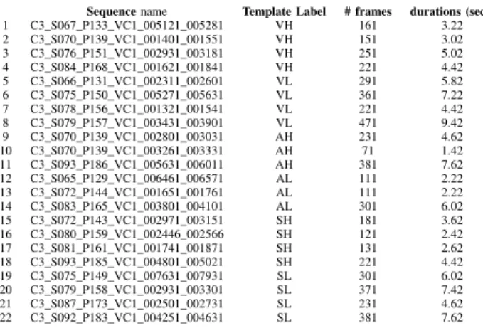
TABLE 1. INFORMATION RELATED TO THE22TEMPLATES FROM THE
SEWA DATABASE CORREPONDING TO THEGERMAN CULTURE(C3),
WHICH ARE USED FOR ALL EXPERIMENTS REPORTED IN THIS PAPER.
Sequencename Template Label # frames durations (secs) 1 C3_S067_P133_VC1_005121_005281 VH 161 3.22 2 C3_S070_P139_VC1_001401_001551 VH 151 3.02 3 C3_S076_P151_VC1_002931_003181 VH 251 5.02 4 C3_S084_P168_VC1_001621_001841 VH 221 4.42 5 C3_S066_P131_VC1_002311_002601 VL 291 5.82 6 C3_S075_P150_VC1_005271_005631 VL 361 7.22 7 C3_S078_P156_VC1_001321_001541 VL 221 4.42 8 C3_S079_P157_VC1_003431_003901 VL 471 9.42 9 C3_S070_P139_VC1_002801_003031 AH 231 4.62 10 C3_S070_P139_VC1_003261_003331 AH 71 1.42 11 C3_S093_P186_VC1_005631_006011 AH 381 7.62 12 C3_S065_P129_VC1_006461_006571 AL 111 2.22 13 C3_S072_P144_VC1_001651_001761 AL 111 2.22 14 C3_S083_P165_VC1_003801_004101 AL 301 6.02 15 C3_S072_P143_VC1_002971_003151 SH 181 3.62 16 C3_S080_P159_VC1_002446_002566 SH 121 2.42 17 C3_S081_P161_VC1_001741_001871 SH 131 2.62 18 C3_S093_P185_VC1_004801_005021 SH 221 4.42 19 C3_S075_P149_VC1_007631_007931 SL 301 6.02 20 C3_S079_P158_VC1_002931_003301 SL 371 7.42 21 C3_S087_P173_VC1_002501_002731 SL 231 4.62 22 C3_S092_P183_VC1_004251_004631 SL 381 7.62
the Hankel matrix structure and approximation error penalty term, respectively, (4) is equivalently written as
min H,Y,E kHk∗+λkW◦Ek1 s.t. ( ˜ Y=Y+E, H=H(Y), ) (5) where the matrix W∈RD×T has been incorporated as a multiplicative weight matrix forE to account for (possibly) missing observations.
Problem 5 is a convex optimization problem and its global optimum can be found relatively easily by using off-the-shelf optimization methods such as the ADMM. To solve 5, we use the ADMM-based solver summarized in Algorithm 1 in [1]. Having recovered the low-rank approximation Hankel matrix H, the system order is set to rank(H)[24]. Subsequently, the system parametersAˆ,Bˆ,Cˆ,Dˆ and the initial state vector ˆ
x0 are estimated by solving a series of systems of linear
equations following [24]. In what follows, we describe how the learned LTI system representation(s) for the observed behavior(s) is (are) used for behavior prediction.
Behavior Prediction.Consider the case where continuous-time, real-valued annotations characterizing dynamic affec-tive behavior (e.g., valence, arousal, liking), manifested in a audio-visual episode of T frames, are available for a number of consecutive frames t = 0,1, . . . , Ttrain−1
(training set). The goal herein is to first learn a low-order LTI system that generates the annotations as outputs Y = [y0,y1, . . . ,yTtrain−1] ∈ R
m×Ttrain when features
act as inputsU= [u0,u1, . . . ,uTtrain−1]∈R
d×Ttrain, and
next use it to predict behavior measurements ˆyt for the
remaining frames of the sequencet=Ttrain, . . . , T−1(test
set), based on the respective features ut. Therefore, having
learned the LDS representation S := Aˆ,Bˆ,Cˆ,Dˆ,ˆx0
for the temporal dynamics of the displayed behavior from the training observations as described above, test set real-valued predictionsˆy(t=Ttrain, . . . , T−1) are obtained by
applying the equations of the learned state-space model (2) fort= 0,1, . . . , Ttrain−1, with the features used as inputs
ut.
4. Data, Features & Protocol
All experiments presented in this paper have been con-ducted on audio-visual episodes from the SEWA Database2 (SEWA DB), a multilingual dataset of richly annotated facial, vocal and verbal behavior recordings in-the-wild (in naturalistic setting). The SEWA DB contains more than 2000 minutes of audio-visual data and includes rich annotations of the recordings in terms of facial landmarks, facial action units (FAU), various vocalizations, verbal cues, mirroring, and rapport, as well as continuous-valued valence, arousal, liking, which this paper focuses on. It also includes behavior templates (segmented episodes) for each culture in which the subjects are in the emotional state of low / high valence (VL/VH), low / high arousal (AL/AH) or showing disliking / liking (SL/SH) in relation to the advertisement.
In this paper, we use all the 22 templates (VL:4,VH:4, AL:3, AH:3,SL:4,SH:4) belonging to the German culture (C3), for behavior prediction experiments. Useful information on the templates is reported in Table 1. Both audio and visual feature sets are downsampled to match the video frame rate, which is 50 frames per second. The mean and standard devi-ation of durdevi-ation over all 22 templates are 4.8 seconds and 2.1 seconds, respectively. For the prediction experiment, we follow [1] and use 70% of each template for training and the remaining 30% for testing. In other words, a different LDS is learned for each the 22 templates based on the training set frames of only one sequence each time and testing on the rest. We use both audio and video features as well as fusion of them. For audio features, we employ the extended Geneva Minimalistic Acoustic Parameter Set (eGEMAPS) [25] which include a compact set of 23 spectral, prosodic and voice quality information and have shown great performance for the modeling of emotion of speech. For video features, we employ geometric features from the face region based on a 49-point markup of facial points tracked with the Chehra facial landmark tracker [26]. In particular, for each video frame we project the 49 facial landmarks on the subspace of a facial shape model, which has been previously created following [27]. Our final video feature vector consists of the first 18 PCA coefficients that account for the 95% of the training set variability. Both audio and visual feature sets are down-sampled to match the video frame rate, which is 50 frames per second. For audio-visual features, we use the feature-level fusion approach and concatenate the two feature vectors for the corresponding time-steps.
Behavior prediction accuracy is measured in terms of the Pearson Correlation Coefficient (COR, measured between the ground truth˜yt annotation and the predicted outputˆyt
on the test set frames (t∈[Ttrain, T−1]) of each sequence.
Experimental results are reported separately for the three behaviors considered herein, that is,Valence, Arousaland Liking, as the median over the CORR values obtained for the test frames of all sequences belonging to each template. The median is preferred over the mean as it is less susceptible to extrema and small sample size.
(a)ValencePrediction Results (b)ArousalPrediction Results (c)LikingPrediction Results
Figure 1.(Better viewed in color). Overall prediction results in terms of correlation (CORR) – measured on the test set frames for each sequence separately – obtained by the proposed predictive framework for the 22 sequences of the SEWA Database belonging to the German culture (C3) representing templates of (a)Valence(median of CORR values over 8 sequences), (b)Arousal(median of CORR values over 6 sequences) and (c)Liking(median of CORR values over 8 sequences), respectively, usingAudio(top row),Video(middle row) andAudio-Visual(bottom row) features. The correlation values are reported in separately bars for each annotation (A: Audio, V:Video, AV: Audio-Visual).
5. Experimental Results
Behavior prediction results obtained by the proposed predictive framework for the 22 sequences of the SEWA Database belonging to the German culture (C3) are shown in Fig. 1 separately for templates of (a) Valence(median of CORR values over 8 sequences), (b) Arousal (median of CORR values over 6 sequences) and (c) Liking(median of CORR values over 8 sequences), respectively, for all three features examined, that is, Audio, Videoand Audio-Visual features. In the bar graph of Fig. 1, the CORR values are reported in separate bars for each annotation (A: Audio, V:Video, AV: Audio-Visual). Note again that for each of the 22 templates a different LDS has been learned based on the training features and annotations, while the CORR values have been measured only in the test frames. For Information on the sequences used in these experiments please refer to Table 1.
The setting of our baseline experiment allows us to investigate the effect of using the audio and video modality and fusion of them on the results. In addition, we are able to separate the effect of culture on the results. As annotations have been performed separately on the basis of the audio, video and audio-video feeds, respectively, but by the same annotators , we are also able to examine the performance of our predictive framework in recognizing the real-valued level of valence, arousal and liking displayed by a subject given each type of information.
As can be seen from the bar graph of Fig. 1a,Valence is more accurately predicted when using audio features in terms of CORR values measured with respect to the video-based ground truth labels (CORR = 0.395), while video features result in rather poor performance. This finding is in discordance with recent evidence suggesting that the face and its deformation appears to be the most informative medium of communicating valence among humans [6]. Nonetheless, we have to take into account that in this study only geometrical features are employed, which might fail to capture subtle tale-telling features (e.g., wrinkles, bulges) informative of valence,
as opposed to appearance-based visual features. [6], [7]. The trend is reversed when it comes toArousalprediction, where visual features along with video-based annotations lead to a high performance of CORR=0.542, with the audio features achieving a much lower CORR=0.222 when using audio-visual-based annotations. This can be partially attributed to the nature of data which contain dyadic conversations on an advertisement that are colored with mostly medium levels of arousal, thus making it easier for both humans and an automated framework to visually detect more extreme and longer in duration arousal displays. Last, the highest perfor-mance onLikingprediction is achieved by employing visual features and audio-visual-based annotations (CORR=0.587). This is an expected behavior considering that the visual modality can reveal richer information on whether or not the subjects feel positively about the advertisement they are discussing on. This conforms to recent experimental findings indicating the informative power of visual features for the similar tasks of (dis)agreement detection [3] and conflict intensity estimation [28]. On the other hand, audio features contain para-linguistic, emotion-related cues that might be ‘misleading’ for the task of liking assessment, which might explain the fact that their inclusion leads to a poorer performance compared to the visual-only system. It is also worth mentioning that liking is the only sentiment out of the three examined herein for which the annotations obtained by using the audio-visual feeds consistently lead to higher performance as compared to that obtained by using the unimodal-based annotations. This can be partially attributed to the higher-level of ambiguity naturally characterizing liking displays and, consequently, the added value brought to the reliability of its human assessment when employing both modalities.
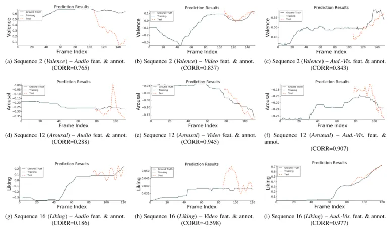
In Fig. 2, line graphs showing the ground truth an-notations along with real-valued behavioral labels for the training and test set frames obtained by the proposed method as a function of the frame index for 3 sequences of the of the SEWA Database (culture: C3 (German)) that have been labeled in terms of in terms of Valence (top row),
(a) Sequence 2 (Valence) –Audiofeat. & annot. (CORR=0.765)
(b) Sequence 2 (Valence) –Videofeat. & annot. (CORR=0.837)
(c) Sequence 2 (Valence) –Aud.-Vis.feat. & annot. (CORR=0.843)
(d) Sequence 12 (Arousal) –Audiofeat. & annot. (CORR=0.288)
(e) Sequence 12 (Arousal) –Videofeat. & annot. (CORR=0.945)
(f) Sequence 12 (Arousal) – Aud.-Vis. feat. & annot.
(CORR=0.907)
(g) Sequence 16 (Liking) –Audiofeat. & annot. (CORR=0.186)
(h) Sequence 16 (Liking) –Videofeat. & annot. (CORR=-0.598)
(i) Sequence 16 (Liking) –Aud.-Vis.feat. & annot. (CORR=0.977)
Figure 2.(Better viewed in color). Continuous-time behavior prediction results in terms ofValence(top row),Arousal(middle row), and Liking(bottom row), respectively, as produced by the proposed predictive framework usingAudio(left),Video(middle) andAudio-Visual features (right), respectively, for 3 templates of the SEWA Database (culture: C3 (German)) that have been annotated based on the annotations produced on the basis of the respective modalities (e.g., theAudioannotations have been obtained by listening to the audio stream). In each graph, the curve labeled asTraining (Test)corresponds to the training (test) predictions, while the third, solid-line curve corresponds to theGround truth annotations.
Arousal(middle row), andLiking(bottom row), respectively. Predictions are illustrated for the three different scenarios of using Audio (left column), Video(middle column) and Audio-Visual features (right column), respectively, for each of which the respective modality has been also used for the human ground truth annotations. For Sequence 2 (Fig. 2a-c), which has been assigned to the template label of VH (high valence), we observe that better results are obtained by using video and audio-visual features compared to the audio features. By carefully inspecting the three different ground truth annotations, we can see that the video-based (V) and audio-visual-based (AV) annotations include much more dynamics patterns and fluctuations, as compared to the audio-based (A) annotation which has a more stationary and thus less informative behavior over time. Hence, it is evident that the former annotations facilitate the linear dynamical system-based modeling obtained by our method leading to systems that can generalize better to unseen observations. For Sequence 12 (Fig. 2d-f), which has been assigned to the template label ofAL(low arousal), the trend is similar, with the video-based system in Fig. 2d offering the highest accuracy of CORR=0.945. It is worth noting that, although the proposed learning method has been presented with
relatively constant arousal values in the training frames and just very few samples of diminishing arousal behavior in the last part of the training set, it manages to predict the downhill of arousal in the test frames of the sequence highly accurately. The audio-visual based system in Fig. 2e, despite achieving a high correlation of 0.907, leads to a more unstable curve for the predicted arousal values, presumably to the annotations containing long portions of almost-constant arousal labels. Lastly, the predictions results for Sequence 16 (Fig. 2g-i), which has been assigned to the template label of SH (high liking), represent a clear example of how feature-level fusion of audio and visual features can help disambiguate subtle sentiment displays like that of liking. While the audio-and video-based frameworks fail to capture the temporal dynamics of the observed behavior, the audio-visual-based system in Fig. 2i achieves a performance of CORR=0.977 on the test frames, despite the fact that the biggest portion of the training set frames are labeled with zero-valued liking and the rest of it including just coarse dynamics of ascending liking. This provides an indication of the effectiveness of our method to efficiently learn the latent dynamics of affective behavior from even a very small amount of annotated training data involving (possibly) unreliable or ‘not rich’ annotations.
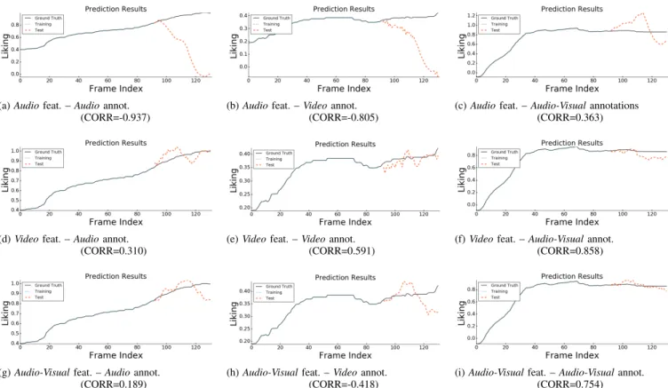
(a)Audiofeat. –Audioannot. (CORR=-0.937)
(b)Audiofeat. –Videoannot. (CORR=-0.805)
(c)Audiofeat. –Audio-Visualannotations (CORR=0.363)
(d)Videofeat. –Audioannot. (CORR=0.310)
(e)Videofeat. –Videoannot. (CORR=0.591)
(f)Videofeat. –Audio-Visualannot. (CORR=0.858)
(g)Audio-Visualfeat. –Audioannot. (CORR=0.189)
(h)Audio-Visualfeat. –Videoannot. (CORR=-0.418)
(i)Audio-Visualfeat. –Audio-Visualannot. (CORR=0.754)
Figure 3.(Better viewed in color). Behavior prediction results as produced by the proposed predictive framework for Sequence 17 (C3_S081_P161_VC1_001741_001871–Low Liking (SL)template) of the SEWA Database (culture:C3(German)) usingAudio(top row), Video(middle row) andAudio-Visual(bottom row) features, respectively, in terms ofLikingthat has been annotated based on theAudio, VideoandAudio-Visualstreams. In each graph, the curve labeled asTraining (Test)corresponds to the training (test) predictions, while the third, solid-line curve corresponds to theGround truthannotations.
The effect of using different annotations and dif-ferent features can be visually inspected by the line graphs illustrated in Fig. 3 which show the ground truth annotations and predicted labels for Sequence 17 (C3_S081_P161_VC1_001741_001871– (Low Liking (SL) template) of the SEWA Database (culture: C3 (German)) separately for all three features and all three annotations examined in our experiments. The subfigures are arranged so that different features vary along rows and different annotations vary across columns. It is evident that the audio-based annotations lead to relatively poor performance for all three features as compared to the remaining two annotations. This is presumably due to the former corresponding to a rather coarse assessment of the observed behavior of liking, which, as highlighted above, is better assessed when the annotators base their measurements on both streams. The remaining results are in accordance with the overall liking prediction results reported in Fig.1c and the related discussion above. The best performance of CORR=0.858 is obtained by the video-based framework trained with audio-visual annotations. It is worth noting that our LDS-based framework manages to predict a trajectory of almost-constant liking labels along the test frames, despite having been ‘presented’ a training trajectory divided into two parts, that is, the first
with (almost)-always-ascending labels and the second with (almost)-constant labels. This behavior is complementary to the behavior observed again for liking prediction in Fig. 2i, where our framework learned from a training set containing again portions of ascending and constant label values, but was capable of correctly predicting a trajectory of ascending labels this time. These two examples jointly suggest the gen-eralization power of the proposed methodology in predicting high-level future values of affective behavior labels even from small amounts of not-much-informative training annotations.
6. Conclusion
A framework for prediction of facial, vocal and audio-visual affective behavior in-the-wild was presented in this paper. The presented framework approaches spontaneous and subtle affective behaviors as smoothly-varying dynamic phenomena expressed in continuous time and scale. In the core of the proposed modeling paradigm lies a generative auto-regressive model which takes the form a linear dynam-ical system generating (possibly) noisy annotations when presented with features and annotations that are corrupted by sparse noise of large magnitude. In this way, a generative model is learned in a supervised way for each displayed
behavior, which is, subsequently, used to predict future mea-surements of behavior for the same sequence. The efficiency of the presented predictive framework was evidenced by conducting experiments on predicting future values affective behavior, namely valence, arousal and liking, manifested in spontaneous dyadic conversations captured in-the-wild. The effect of employing facial, vocal or audio-visual features as well as annotations having been generated on the basis of all those streams is also investigated systematically, separately for each affective behavior. Our results demonstrate that spontaneous and thus highly-ambiguous affective behavior can be predicted with high accuracy from a uni-modal or a multi-modal approach, better suited to the sentiment in question, even from small training sets, hence with minimal annotation, by relying on robust sequential learning.
Acknowledgment
This work is funded by the European Community Horizon 2020 [H2020/2014-2020] under grant agreement no. 645094 (SEWA).
References
[1] C. Georgakis, Y. Panagakis, and M. Pantic, “Dynamic behavior analysis via structured rank minimization,” International Journal of Computer Vision, pp. 1–25, 2017. [Online]. Available: http: //dx.doi.org/10.1007/s11263-016-0985-3
[2] H. Wang, M. M. Ullah, A. Klaser, I. Laptev, and C. Schmid, “Evaluation of local spatio-temporal features for action recognition,” inBMVC 2009-British Machine Vision Conference. BMVA Press, 2009, pp. 124–1.
[3] K. Bousmalis, M. Mehu, and M. Pantic, “Spotting agreement and disagreement: A survey of nonverbal audiovisual cues and tools,” in
IEEE International Conference on Affective Computing and Intelligent Interaction and Workshops, 2009, pp. 1–9.
[4] I. Cohen, N. Sebe, A. Garg, L. S. Chen, and T. S. Huang, “Facial expression recognition from video sequences: temporal and static modeling,”Computer Vision and Image Understanding, vol. 91, no. 1, pp. 160–187, 2003.
[5] S. Kim, F. Valente, M. Filippone, and A. Vinciarelli, “Predicting Continuous Conflict Perception with Bayesian Gaussian Processes,”
IEEE Transactions on Affective Computing, vol. 5, no. 2, pp. 187–200, 2014.
[6] H. Gunes and B. Schuller, “Categorical and dimensional affect analysis in continuous input: Current trends and future directions,”Image and Vision Computing, vol. 31, no. 2, pp. 120–136, 2013.
[7] M. A. Nicolaou, H. Gunes, and M. Pantic, “Continuous Prediction of Spontaneous Affect from Multiple Cues and Modalities in Valence-Arousal Space,”IEEE Transactions on Affective Computing, pp. 92– 105, 2011.
[8] Z. Ambadar, J. W. Schooler, and J. F. Cohn, “Deciphering the enigmatic face the importance of facial dynamics in interpreting subtle facial expressions,”Psychological science, vol. 16, no. 5, pp. 403–410, 2005.
[9] M. Pantic,Facial Expression Recognition, 2014, pp. 1–8.
[10] P. Ekman, “Darwin, deception, and facial expression,”Annals of the New York Academy of Sciences, vol. 1000, no. 1, pp. 205–221, 2003. [11] Y. Panagakis, M. A. Nicolaou, S. Zafeiriou, and M. Pantic, “Robust
Correlated and Individual Component Analysis,”IEEE Transactions on Pattern Analysis and Machine Intelligence (TPAMI), Special Issue in Multimodal Pose Estimation and Behaviour Analysis, (accepted), 2016.
[12] M. A. Nicolaou, V. Pavlovic, and M. Pantic, “Dynamic Probabilistic CCA for Analysis of Affective Behaviour and Fusion of Continuous Annotations,”IEEE Transactions on Pattern Analysis and Machine Intelligence, vol. 36, no. 7, pp. 1299–1311, 2014.
[13] M. Fazel, T. K. Pong, D. Sun, and P. Tseng, “Hankel matrix rank minimization with applications to system identification and realization,”
SIAM Journal on Matrix Analysis and Applications, vol. 34, no. 3, pp. 946–977, 2013.
[14] R. D. Lane and L. Nadel,Cognitive neuroscience of emotion. Oxford University Press, USA, 2002.
[15] M. A. Nicolaou, H. Gunes, and M. Pantic, “Output-associative rvm regression for dimensional and continuous emotion prediction,”Image and Vision Computing, vol. 30, no. 3, pp. 186–196, 2012.
[16] M. Wöllmer, F. Eyben, S. Reiter, B. W. Schuller, C. Cox, E. Douglas-Cowie, R. Cowieet al., “Abandoning emotion classes-towards contin-uous emotion recognition with modelling of long-range dependencies.” inInterspeech, vol. 2008, 2008, pp. 597–600.
[17] T. Baltrusaitis, N. Banda, and P. Robinson, “Dimensional affect recognition using continuous conditional random fields,” inIEEE International Conference and Workshops on Automatic Face and Gesture Recognition (FG), 2013, pp. 1–8.
[18] V. Pavlovi´c, J. M. Rehg, T.-J. Cham, and K. P. Murphy, “A dynamic bayesian network approach to figure tracking using learned dynamic models,” in IEEE International Conference on Computer Vision (ICCV), vol. 1, 1999, pp. 94–101.
[19] K. Bousmalis, S. Zafeiriou, L.-P. Morency, and M. Pantic, “Infinite hidden conditional random fields for human behavior analysis,”IEEE transactions on neural networks and learning systems, vol. 24, no. 1, pp. 170–177, 2013.
[20] L. Vandenberghe and S. Boyd, “Semidefinite programming,”SIAM review, vol. 38, no. 1, pp. 49–95, 1996.
[21] B. K. Natarajan, “Sparse approximate solutions to linear systems,”
SIAM journal on computing, vol. 24, no. 2, pp. 227–234, 1995. [22] M. Fazel, H. Hindi, and S. P. Boyd, “A rank minimization heuristic
with application to minimum order system approximation,” in Ameri-can Control Conference, 2001. Proceedings of the 2001, vol. 6. IEEE, 2001, pp. 4734–4739.
[23] D. L. Donoho, “For most large underdetermined systems of linear equations the minimal 1-norm solution is also the sparsest solution,”
Communications on pure and applied mathematics, vol. 59, no. 6, pp. 797–829, 2006.
[24] P. Van Overschee and B. De Moor,Subspace identification for linear systems: Theory—Implementation—Applications. Springer Science & Business Media, 2012.
[25] M. Valstar, J. Gratch, B. Schuller, F. Ringeval, D. Lalanne, M. Tor-res TorTor-res, S. Scherer, G. Stratou, R. Cowie, and M. Pantic, “Avec 2016: Depression, mood, and emotion recognition workshop and challenge,” inProceedings of the 6th International Workshop on Audio/Visual Emotion Challenge. ACM, 2016, pp. 3–10.
[26] A. Asthana, S. Zafeiriou, G. Tzimiropoulos, S. Cheng, and M. Pantic, “From pixels to response maps: Discriminative image filtering for face alignment in the wild,”IEEE transactions on pattern analysis and machine intelligence, vol. 37, no. 6, pp. 1312–1320, 2015. [27] G. Chrysos, E. Antonakos, S. Zafeiriou, and P. Snape, “Offline
Deformable Face Tracking in Arbitrary Videos,” inProceedings of IEEE International Conference on Computer Vision, 300 Videos in the Wild (300-VW): Facial Landmark Tracking in-the-Wild Challenge & Workshop (ICCVW’15), Santiago, Chile, December 2015. [28] C. Georgakis, Y. Panagakis, S. Zafeiriou, and M. Pantic, “The conflict
escalation resolution (confer) database,”Image and Vision Computing, 2017.