Data Mining via Support Vector Machines

Data Mining via Support Vector Machines

O. L. Mangasarian

Computer Sciences Department

University of Wisconsin

1210 West Dayton Street

Madison, WI 53706

Abstract

Support vector machines (SVMs) have played a key role in broad classes of problems arising in various fields. Much more recently, SVMs have become the tool of choice for problems arising in data classifi-cation and mining. This paper emphasizes some recent developments that the author and his colleagues have contributed to such as: gen-eralized SVMs (a very general mathematical programming framework for SVMs), smooth SVMs (a smooth nonlinear equation representation of SVMs solvable by a fast Newton method), Lagrangian SVMs (an unconstrained Lagrangian representation of SVMs leading to an ex-tremely simple iterative scheme capable of solving classification prob-lems with millions of points) and reduced SVMs (a rectangular kernel classifier that utilizes as little as 1% of the data).

1

Introduction

This paper describes four recent developments, one theoretical, three algo-rithmic, all centered on support vector machines (SVMs). SVMs have be-come the tool of choice for the fundamental classification problem of machine learning and data mining. We briefly outline these four developments now.

In Section 2 new formulations for SVMs are given as convex mathemati-cal programs which are often quadratic or linear programs. By setting apart

the two functions of a support vector machine: separation of points by a nonlinear surface in the original space of patterns, and maximizing the dis-tance between separating planes in a higher dimensional space, we are able to define indefinite, possibly discontinuous, kernels, not necessarily inner prod-uct ones, that generate highly nonlinear separating surfaces. Maximizing the distance between the separating planes in the higher dimensional space is sur-rogated by support vector suppression, which is achieved by minimizing any desired norm of support vector multipliers. The norm may be one induced by the separation kernel if it happens to be positive definite, or a Euclidean or a polyhedral norm. The latter norm leads to a linear program whereas the former norms lead to convex quadratic programs, all with an arbitrary separation kernel. A standard support vector machine can be recovered by using the same kernel for separation and support vector suppression.

In Section 3 we apply smoothing methods, extensively used for solving important mathematical programming problems and applications, to gen-erate and solve an unconstrained smooth reformulation of the support vec-tor machine for pattern classification using a completely arbitrary kernel. We term such reformulation a smooth support vector machine (SSVM). A fast Newton-Armijo algorithm for solving the SSVM converges globally and quadratically. Numerical results and comparisons demonstrate the effective-ness and speed of the algorithm. For example, on six publicly available datasets, tenfold cross validation correctness of SSVM was the highest com-pared with four other methods as well as the fastest.

In Section 4 an implicit Lagrangian for the dual of a simple reformula-tion of the standard quadratic program of a linear support vector machine is proposed. This leads to the minimization of an unconstrained differentiable convex function in a space of dimensionality equal to the number of classified points. This problem is solvable by an extremely simple linearly convergent Lagrangian support vector machine (LSVM) algorithm. LSVM requires the inversion at the outset of a single matrix of the order of the much smaller di-mensionality of the original input space plus one. The full algorithm is given in this paper in 11 lines of MATLAB code without any special optimization tools such as linear or quadratic programming solvers. This LSVM code can be used “as is” to solve classification problems with millions of points.

In Section 5 an algorithm is proposed which generates a nonlinear kernel-based separating surface that requires as little as 1% of a large dataset for its explicit evaluation. To generate this nonlinear surface, the entiredataset is used as a constraint in an optimization problem with very few variables

corresponding to the 1% of the data kept. The remainder of the data can be thrown away after solving the optimization problem. This is achieved by making use of a rectangular m×m¯ kernel K(A,A¯0_{) that greatly reduces the}

size of the quadratic program to be solved and simplifies the characterization of the nonlinear separating surface. Here, the m rows of A represent the original m data points while the ¯m rows of ¯A represent a greatly reduced

¯

m data points. Computational results indicate that test set correctness for the reduced support vector machine (RSVM), with a nonlinear separating surface that depends on a small randomly selected portion of the dataset, is better than that of a conventional support vector machine (SVM) with a nonlinear surface that explicitly depends on the entire dataset, and much better than a conventional SVM using a small random sample of the data. Computational times, as well as memory usage, are much smaller for RSVM than that of a conventional SVM using the entire dataset.

A word about our notation. All vectors will be column vectors unless transposed to a row vector by a prime superscript 0_{. For a vector x in the}

n-dimensional real space Rn_{, the plus function x}

+ is defined as (x+)i =

max {0, xi}, i = 1, . . . , n, while x∗ denotes the step function defined as

(x∗)i = 1 if xi >0 and (x∗)i = 0 if xi ≤0, i = 1, . . . , n. The scalar (inner)

product of two vectors x and y in the n-dimensional real space Rn _{will be}

denoted by x0y and the p-norm of x will be denoted by kxkp. If x0y = 0, we than write x ⊥y. For a matrix A∈ Rm×n_{, A}

i is the ith row of A which

is a row vector in Rn_{. A column vector of ones of arbitrary dimension will}

be denoted by e. For A ∈ Rm×n _{and B ∈ R}n×l_{, the kernel K(A, B) maps}

Rm×n_×Rn×l _{into R}m×l_{. In particular, if x and y are column vectors in R}n

then,K(x0_{, y) is a real number,K(x}0_{, A}0_{) is a row vector inR}m _{andK(A, A}0₎

is anm×mmatrix. Iffis a real valued function defined on then-dimensional real space Rn_{, the gradient of f at x is denoted by ∇f(x) which is a row}

vector in Rn _{and the n×n Hessian matrix of second partial derivatives of f}

atxis denoted by∇2_{f(x). The base of the natural logarithm will be denoted}

2

The Generalized Support Vector Machine

(GSVM) [25]

We consider the problem of classifying m points in the n-dimensional real space Rn_{, represented by the m×n matrix A, according to membership of}

each point Ai in the classes +1 or -1 as specified by a given m×m diagonal

matrix D with ones or minus ones along its diagonal. For this problem the standard support vector machine with a linear kernel AA0 _{[38, 11] is given}

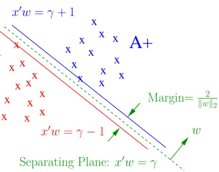
by the following for some ν >0: min (w,γ,y)∈Rn+1+m νe 0_y+1 2w0w s.t. D(Aw−eγ) +y ≥ e y ≥ 0. (1)

Here w is the normal to the bounding planes:

x0_{w − γ = +1}

x0_{w − γ = −1,} (2)

and γ determines their location relative to the origin. The first plane above bounds the class +1 points and the second plane bounds the class -1 points when the two classes are strictly linearly separable, that is when the slack variable y= 0. The linear separating surface is the plane

x0w=γ, (3)

midway between the bounding planes (2). See Figure 1. If the classes are linearly inseparable then the two planes bound the two classes with a “soft margin” determined by a nonnegative slack variable y, that is:

x0_{w − γ + y}

i ≥ +1, forx0 =Ai andDii= +1,

x0_{w − γ − y}

i ≤ −1, forx0 =Ai and Dii =−1. (4)

The 1-norm of the slack variable y is minimized with weight ν in (1). The quadratic term in (1), which is twice the reciprocal of the square of the 2-norm distance _kw2_k2 between the two bounding planes of (2) in the n-dimensional space of w ∈ Rn _{for a fixed γ, maximizes that distance, often called the}

“margin”. Figure 1 depicts the points represented byA, the bounding planes (2) with margin _kw2_k2, and the separating plane (3) which separates A+,

x

x

x

x

x

x

x

x

x

x

x

x

x

x

x

x

x

x

x

x

x

x

x

x

x

x

A+

w

Margin=

x

w

=

γ

−

1

x

w

=

γ

+ 1

Separating Plane:

x

w

=

γ

Figure 1: The bounding planes (2) with margin 2

kwk2, and the plane (3)

sep-arating A+, the points represented by rows of A with Dii = +1, from A−, the

points represented by rows of A with Dii=−1.

the points represented by rows of A with Dii = +1, from A−, the points

represented by rows of A with Dii =−1.

In the GSVM formulation we attempt to discriminate between the classes +1 and -1 by a nonlinear separating surface which subsumes the linear sep-arating surface (3), and is induced by some kernel K(A, A0_{), as follows:}

K(x0_{, A}0_{)Du=γ, (5)}

where K(x0_{, A}0_)∈Rm_{,e.g. K(x}0_{, A}0_{) =x}0_{A for the linear separating surface}

(3) and w = A0_{Du. The parameters u ∈ R}m _{and γ ∈ R are determined}

by solving a mathematical program, typically quadratic or linear. In special cases, such as the standard SVM (13) below, u can be interpreted as a dual variable. A point x∈Rn _{is classified in class +1 or -1 according to whether}

the decision function

(K(x0, A0)Du−γ)∗, (6)

yields 1 or 0 respectively. Here (·)∗ denotes the step function defined in the

map from x ∈ Rn _{to some other space z ∈ R}k _{where k may be much larger}

thann. In particular if the kernelKis an inner product kernel under Mercer’s condition [13, pp 138-140],[38, 11, 5] (an assumption that we will not make in this paper) then for x and y inRn_:

K(x, y) =h(x)0h(y), (7) and the separating surface (5) becomes:

h(x)0_h(A0_{)Du=γ, (8)}

where h is a function, not easily computable, from Rn _{to R}k_{, and h(A}0_{) ∈}

Rk×m _{results from applyinghto them columns ofA}0_{. The difficulty in}

com-puting h and the possible high dimensionality of Rk _{have been important}

factors in using a kernel K as a generator of an implicit nonlinear separating surface in the original feature space Rn _{but which is linear in the high}

di-mensional space Rk_{. Our separating surface (5) written in terms of a kernel}

function retains this advantage and is linear in its parameters, u, γ. We now state a mathematical program that generates such a surface for a general kernel K as follows: min u,γ,y νe 0_y+f(u) s.t. D(K(A, A0_{)Du−eγ) +y ≥ e} y ≥ 0. (9)

Here f is some convex function on Rm_{, typically some norm or seminorm,}

and νis some positive parameter that weights the separation errore0_yversus

suppression of the separating surface parameter u. Suppression of u can be interpreted in one of two ways. We interpret it here as minimizing the number of support vectors, i.e. constraints of (9) with positive multipliers. A more conventional interpretation is that of maximizing some measure of the distance or margin between the bounding parallel planes in Rk_{, under}

appropriate assumptions, such as f being a quadratic function induced by a positive definite kernel K as in (13) below. As is well known, this leads to improved generalization by minimizing an upper bound on the VC dimension [38, 35].

We term a solution of the mathematical program (9) and the resulting decision function (6) a generalized support vector machine, GSVM. In what follows derive a number of special cases, including the standard support vector machine.

We consider first support vector machines that include the standard ones [38, 11, 5] and which are obtained by settingf of (9) to be a convex quadratic function f(u) = 1₂u0_{Hu, where H ∈ R}m×m _{is some symmetric positive}

def-inite matrix. The mathematical program (9) becomes the following convex quadratic program: min u,γ,y νe 0_y+1 2u 0_Hu s.t. D(K(A, A0_{)Du−eγ) +y ≥ e} y ≥ 0. (10)

The Wolfe dual [39, 22] of this convex quadratic program is: min r∈Rm 1 2r 0_{DK(A, A}0_)DH−1_{DK(A, A}0₎0_Dr−e0_r s.t. e0_{Dr = 0} 0≤r ≤ νe. (11)

Furthermore, the primal variable u is related to the dual variable r by:

u=H−1DK(A, A0)0Dr. (12) If we assume that the kernel K(A, A0_{) is symmetric positive definite and}

let H = DK(A, A0_{)D, then our dual problem (11) degenerates to the dual}

problem of the standard support vector machine [38, 11, 5] with u=r: min u∈Rm 1 2u0DK(A, A0)Du−e0u s.t. e0Du = 0 0≤u ≤ νe. (13)

The positive definiteness assumption on K(A, A0_{) in (13) can be relaxed to}

positive semidefiniteness while maintaining the convex quadratic program (10), with H = DK(A, A0_{)D, as the direct dual of (13) without utilizing}

(11) and (12). The symmetry and positive semidefiniteness of the kernel

K(A, A0_{) for this version of a support vector machine is consistent with the}

support vector machine literature. The fact that r = u in the dual formu-lation (13), shows that the variable u appearing in the original formulation (10) is also the dual multiplier vector for the first set of constraints of (10). Hence the quadratic term in the objective function of (10) can be thought of as suppressing as many multipliers of support vectors as possible and thus

minimizing the number of such support vectors. This is another (nonstan-dard) interpretation of the standard support vector machine that is usually interpreted as maximizing the margin or distance between parallel separating planes.

This leads to the idea of using other values for the matrix H other than

DK(A, A0_{)D that will also suppress u. One particular choice is interesting}

because it puts no restrictions on K: no symmetry, no positive definiteness or semidefiniteness and not even continuity. This is the choice H =I in (10) which leads to a dual problem (11) with H = I and u = DK(A, A0₎0_{Dr as}

follows: min r∈Rm 1 2r0DK(A, A0)K(A, A0)0Dr−e0r s.t. e0_{Dr = 0} 0≤r ≤ νe. (14)

We note immediately that K(A, A0_{)K(A, A}0₎0 _{is positive semidefinite with}

no assumptions on K(A, A0_{), and hence the above problem is an always}

solvable convex quadratic program for any kernel K(A, A0_{). In fact by the}

Frank-Wolfe existence theorem [15], the quadratic program (10) is solvable for any symmetric positive definite matrix H because its objective function is bounded below by zero. Hence by quadratic programming duality its dual problem (11) is also solvable. Any solution of (10) can be used to generate a nonlinear decision function (6). Thus we are free to choose any symmetric positive definite matrix H to generate a support vector machine. Experimentation will be needed to determine what are the most appropriate choices for H.

By using the 1-norm instead of the 2-norm a linear programming for-mulation for the GSVM can be obtained. We refer the interested reader to [25].

We turn our attention now to an efficient method for generating SVMs based on smoothing ideas that have already been effectively used to solve various mathematical programs [7, 8, 6, 9, 10, 16, 37, 12].

3

SSVM: Smooth Support Vector Machines

[21]

In our smooth approach, the square of 2-norm of the slack variable y is minimized with weight ν

the distance between the planes (2) is measured in the (n+ 1)-dimensional space of (w, γ)∈Rn+1_{, that is} 2

k(w,γ)k2. Measuring the margin in this (n+

1)-dimensional space instead of Rn _{induces strong convexity and has little or no}

effect on the problem as was shown in [27, 29, 21, 20]. Thus using twice the reciprocal squared of this margin instead, yields our modified SVM problem as follows: min w,γ,y ν 2y0y+ 1 2(w0w+γ2) s.t. D(Aw−eγ) +y ≥ e y ≥ 0. (15)

At the solution of problem (15), y is given by

y= (e−D(Aw−eγ))+, (16)

where, as defined in the Introduction, (·)+ replaces negative components of

a vector by zeros. Thus, we can replace y in (15) by (e−D(Aw−eγ))+

and convert the SVM problem (15) into an equivalent SVM which is an unconstrained optimization problem as follows:

min w,γ ν 2k(e−D(Aw−eγ))+k 2 2+12(w 0_w+γ2_). (17) This problem is a strongly convex minimization problem without any con-straints. It is easy to show that it has a unique solution. However, the objective function in (17) is not twice differentiable which precludes the use of a fast Newton method. We thus apply the smoothing techniques of [7, 8] and replace x+ by a very accurate smooth approximation [21, Lemma 2.1]

that is given byp(x, α), the integral of the sigmoid function 1

1+ε−αx of neural networks [23], that is

p(x, α) =x+ 1

αlog(1 +ε

−αx_{), α >0. (18)}

This p function with a smoothing parameter α is used here to replace the plus function of (17) to obtain a smooth support vector machine (SSVM):

min (w,γ)∈Rn+1Φα(w, γ) := _(w,γmin_)∈Rn+1 ν 2kp(e−D(Aw−eγ), α)k 2 2+ 1 2(w 0_w+γ2_). (19) It can be shown [21, Theorem 2.2] that the solution of problem (15) is ob-tained by solving problem (19) with α approaching infinity. Advantage can

be taken of the twice differentiable property of the objective function of (19) to utilize a quadratically convergent algorithm for solving the smooth support vector machine (19) as follows.

Algorithm 3.1 Newton-Armijo Algorithm for SSVM (19)

Start with any (w0_{, γ}0_{) ∈ R}n+1_{. Having (w}i_{, γ}i_{), stop if the gradient of the}

objective function of (19) is zero, that is ∇Φα(wi, γi) = 0. Else compute

(wi+1_{, γ}i+1_{) as follows:}

(i) Newton Direction: Determine direction di _{∈ R}n+1 _{by setting equal}

to zero the linearization of∇Φα(w, γ) around (wi, γi) which givesn+ 1

linear equations in n+ 1 variables:

∇2Φα(wi, γi)di =−∇Φα(wi, γi)0. (20)

(ii) Armijo Stepsize [1]: Choose a stepsize λi ∈R such that:

(wi+1, γi+1) = (wi, γi) +λidi (21)

where λi = max{1,1₂,1₄, . . .} such that :

Φα(wi, γi)−Φα((wi, γi) +λidi)≥ −δλi∇Φα(wi, γi)di (22)

where δ∈(0,1 2).

Note that a key difference between our smoothing approach and that of the classical SVM [38, 11] is that we are solving here a linear system of equations (20) instead of solving a quadratic program as is the case with the classical SVM. Furthermore, it can be shown [21, Theorem 3.2] that the smoothing algorithm above converges quadratically from any starting point. To obtain a nonlinear SSVM we consider the GSVM formulation (9) with a 2-norm squared error term on y instead of the 1-norm, and instead of the convex term f(u) that suppresses u we use a 2-norm squared of u

γ

to suppress both u and γ. We obtain then:

min u,γ,y ν 2y 0_y+ 1 2(u 0_u+γ2₎ s.t. D(K(A, A0_{)Du−eγ) +y ≥ e} y ≥ 0. (23)

We repeat the same arguments as above, in going from (15) to (19), to obtain the SSVM with a nonlinear kernel K(A, A0_):

min u,γ ν 2kp(e−D(K(A, A 0_{)Du−eγ), α)k}2 2+ 12(u 0_u+γ2_), (24)

where K(A, A0_{) is a kernel map from R}m×n _×Rn×m _{to R}m×m_{. We note}

that this problem, which is capable of generating highly nonlinear separating surfaces, still retains the strong convexity and differentiability properties for any arbitrary kernel. All of the convergence results for a linear kernel hold here for a nonlinear kernel [21].

The effectiveness and speed of the smooth support vector machine (SSVM) approach can be demonstrated by comparing it numerically with other meth-ods. In order to evaluate how well each algorithm generalizes to future data, tenfold cross-validation is performed on each dataset [36]. To evaluate the efficacy of SSVM, computational times of SSVM were compared with robust linear program (RLP) algorithm [2], the feature selection concave minimiza-tion (FSV) algorithm, the support vector machine using the 1-norm approach (SVMk·k1) and the classical support vector machine (SVMk·k2₂) [3, 38, 11]. All

tests were run on six publicly available datasets: the Wisconsin Prognos-tic Breast Cancer Database [31] and four datasets from the Irvine Machine Learning Database Repository [34]. It turned out that tenfold testing cor-rectness of the SSVM was the highest for these five methods on all datasets tested as well as the computational speed. Detailed numerical results are given in [21].

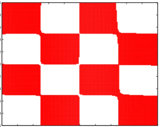
As a test of effectiveness of the SSVM in generating a highly nonlinear separating surface, we tested it on the 1000-point checkerboard dataset of [19] depicted in Figure 2. We used the following a Gaussian kernel in the SSVM formulation (24):

Gaussian Kernel : ε−µkAi−Ajk22, i, j= 1,2,3. . . m.

The value of the parameter µ used as well as values of the parameters ν

and α of the nonlinear SSVM (24) are all given in Figure 3 which depicts the separation obtained. Note that the boundaries of the checkerboard are as sharp as those of [27], obtained by a linear programming solution, and considerably sharper than those of [19], obtained by a Newton approach applied to a quadratic programming formulation.

We turn now to an extremely simple iterative algorithm for SVMs that requires neither a quadratic program nor a linear program to be solved.

0 20 40 60 80 100 120 140 160 180 200 0 20 40 60 80 100 120 140 160 180 200

Figure 2: Checkerboard training dataset

0 20 40 60 80 100 120 140 160 180 200 0 20 40 60 80 100 120 140 160 180 200

Figure 3: Gaussian kernel separation of checkerboard dataset (ν = 10, α = 5, µ= 2)

4

LSVM: Lagrangian Support Vector Machines

[28]

We propose here an algorithm based on an implicit Lagrangian of the dual of a simple reformulation of the standard quadratic program of a linear support vector machine. This leads to the minimization of an unconstrained differ-entiable convex function in a space of dimensionality equal to the number of classified points. This problem is solvable by an extremely simple linearly convergent Lagrangian support vector machine (LSVM) algorithm. LSVM requires the inversion at the outset of a single matrix of the order of the much smaller dimensionality of the original input space plus one. The full algo-rithm is given in this paper in 11 lines of MATLAB code without any special optimization tools such as linear or quadratic programming solvers. This LSVM code can be used “as is” to solve classification problems with millions of points. For example, 2 million points in 10 dimensional input space were classified by a linear surface in 6.7 minutes on a 250-MHz UltraSPARC II [28].

The starting point for LSVM is the primal quadratic formulation (15) of the SVM problem. Taking the dual [24] of this problem gives:

min 0≤u∈Rm 1 2u 0₍I ν +D(AA 0_+ee0_)D)u−e0_{u. (25)}

The variables (w, γ) of the primal problem which determine the separating surface x0_{w = γ are recovered directly from the solution of the dual (25)}

above by the relations:

w=A0Du, y= u

ν, γ =−e

0_{Du. (26)}

We immediately note that the matrix appearing in the dual objective function is positive definite and that there is no equality constraint and no upper bound on the dual variable u. The only constraint present is a nonnegativity one. These facts lead us to our simple iterative Lagrangian SVM Algorithm which requires the inversion of a positive definite (n+ 1)×

(n+1) matrix, at the beginning of the algorithm followed by a straightforward linearly convergent iterative scheme that requires no optimization package.

Before stating our algorithm we define two matrices to simplify notation as follows:

H =D[A −e], Q= I

ν +HH

With these definitions the dual problem (25) becomes min 0≤u∈Rmf(u) := 1 2u 0_Qu−e0_{u. (28)}

It will be understood that within the LSVM Algorithm, the single time that

Q−1 _{is computed at the outset of the algorithm, the SMW identity [17] will}

be used: (I ν +HH 0₎−1 _{=ν(I −H(}I ν +H 0_H)−1_H0_{), (29)}

where ν is a positive number and H is an arbitrary m×k matrix. Hence only an (n+ 1)×(n+ 1) matrix is inverted.

The LSVM Algorithm is based directly on the Karush-Kuhn-Tucker nec-essary and sufficient optimality conditions [24, KTP 7.2.4, page 94] for the dual problem (28) which are the following:

0≤u ⊥ Qu−e≥0. (30)

By using the easily established identity between any two real numbers (or vectors) a and b:

0≤a ⊥ b≥0 ⇐⇒ a= (a−αb)+, α >0, (31)

the optimality condition (30) can be written in the following equivalent form for any positive α:

Qu−e= ((Qu−e)−αu)+. (32)

These optimality conditions lead to the following very simple iterative scheme which constitutes our LSVM Algorithm:

ui+1 _=Q−1_{(e+ ((Qu}i_−e)−αui₎

+), i= 0,1, . . . , (33)

for which we will establish global linear convergence from any starting point under the easily satisfiable condition:

0< α < 2

ν. (34)

We implement this condition as α = 1.9/ν in all our experiments, where ν

is the parameter of our SVM formulation (25). It turns out, and this is the way that led us to this iterative scheme, that the optimality condition (32),

is also the necessary and sufficient condition for the unconstrained minimum of the implicit Lagrangian [30] associated with the dual problem (28):

min u∈RmL(u, α) = min_u∈Rm 1 2u 0_Qu−e0_u+ 1 2α(k(−αu+Qu−e)+k 2 _{− kQu−ek}2_). (35) Setting the gradient with respect to u of this convex and differentiable La-grangian to zero gives

(Qu−e) + 1 α(Q−αI)((Q−αI)u−e)+− 1 αQ(Qu−e) = 0, (36) or equivalently: (αI −Q)((Qu−e)−((Q−αI)u−e)+) = 0, (37)

which is equivalent to the optimality condition (32) under the assumption that α is positive and not an eigenvalue of Q.

In [28] global linear convergence of the iteration (33) under condition (34) is established as follows.

Algorithm 4.1 LSVM Algorithm & Its Global Convergence [28] Let

Q ∈ Rm×m _{be the symmetric positive definite matrix defined by (27) and}

let (34) hold. Starting with an arbitrary u0 _{∈ R}m_{, the iterates u}i _{of (33)}

converge to the unique solution u¯ of (28) at the linear rate:

kQui+1_{−Qu¯k ≤ kI−αQ}−1_{k · kQu}i_{−Qu¯k. (38)}

A complete MATLAB [32] code of LSVM which is capable of solving problems with millions of points using only native MATLAB commands is given below in Code 4.2. The input parameters, besides A, D and ν of (27), which define the problem, are: itmax, the maximum number of iterations and tol, the tolerated nonzero error in kui+1_−ui_{k at termination which can}

be shown [28] to constitute a bound on the distance to the unique solution of the problem from the current iterate.

Code 4.2 LSVM MATLAB Code

function [it, opt, w, gamma] = svml(A,D,nu,itmax,tol) % lsvm with SMW for min 1/2*u’*Q*u-e’*u s.t. u=>0, % Q=I/nu+H*H’, H=D[A -e]

% Input: A, D, nu, itmax, tol; Output: it, opt, w, gamma % [it, opt, w, gamma] = svml(A,D,nu,itmax,tol);

[m,n]=size(A);alpha=1.9/nu;e=ones(m,1);H=D*[A -e];it=0; S=H*inv((speye(n+1)/nu+H’*H));

u=nu*(1-S*(H’*e));oldu=u+1;

while it<itmax & norm(oldu-u)>tol

z=(1+pl(((u/nu+H*(H’*u))-alpha*u)-1)); oldu=u; u=nu*(z-S*(H’*z)); it=it+1; end; opt=norm(u-oldu);w=A’*D*u;gamma=-e’*D*u; function pl = pl(x); pl = (abs(x)+x)/2;

Using this MATLAB code, 2 million random points in 10-dimensional space were classified in 6.7 minutes in 6 iterations to e−5 accuracy using a 250-MHz UltraSPARC II with 2 gigabyte memory. In contrast a linear pro-gramming formulation using CPLEX [14] ran out of memory. Other favorable numerical comparisons with other methods are contained in [28].

We turn now to our final topic of extracting very effective classifiers from a minimal portion of a large dataset.

5

RSVM: Reduced Support Vector Machines

[20]

In this section we describe an algorithm that generates a nonlinear kernel-based separating surface which requires as little as 1% of a large dataset for its explicit evaluation. To generate this nonlinear surface, the entiredataset is used as a constraint in an optimization problem with very few variables corresponding to the 1% of the data kept. The remainder of the data can be thrown away after solving the optimization problem. This is achieved by

making use of a rectangular m×m¯ kernel K(A,A¯0_{) that greatly reduces the}

size of the quadratic program to be solved and simplifies the characterization of the nonlinear separating surface. Here as before, themrows ofArepresent the originalm data points while the ¯mrows of ¯A represent a greatly reduced

¯

m data points. Computational results indicate that test set correctness for the reduced support vector machine (RSVM), with a nonlinear separating surface that depends on a small randomly selected portion of the dataset, is better than that of a conventional support vector machine (SVM) with a nonlinear surface that explicitly depends on the entire dataset, and much better than a conventional SVM using a small random sample of the data. Computational times, as well as memory usage, are much smaller for RSVM than that of a conventional SVM using the entire dataset.

The motivation for RSVM comes from the practical objective of generat-ing a nonlinear separatgenerat-ing surface (5) for a large dataset which uses only a small portion of the dataset for its characterization. The difficulty in using nonlinear kernels on large datasets is twofold. First, there is the computa-tional difficulty in solving the the potentially huge unconstrained optimiza-tion problem (24) which involves the kernel funcoptimiza-tion K(A, A0_{) that typically}

leads to the computer running out of memory even before beginning the so-lution process. For example, for the Adult dataset with 32562 points, which is actually solved with RSVM [20], this would mean a matrix with over one billion entries for a conventional SVM. The second difficulty comes from uti-lizing the formula (5) for the separating surface on a new unseen pointx. The formula dictates that we store and utilize the entire data set represented by the 32562×123 matrix Awhich may be prohibitively expensive storage-wise and computing-time-wise. For example for the Adult dataset just mentioned which has an input space of 123 dimensions, this would mean that the non-linear surface (5) requires a storage capacity for 4,005,126 numbers. To avoid all these difficulties and based on experience with chunking methods [4, 26], we hit upon the idea of using a very small random subset of the dataset given by ¯m points of the original m data points with ¯m << m, that we call

¯

A and use ¯A0 _{in place ofA}0 _{inboth the unconstrained optimization problem}

(24), to cut problem size and computation time, and for the same purposes in evaluating the nonlinear surface (5). Note that the matrix Ais left intact inK(A,A¯0_{), whereas ¯A}0 _{has replacedA}0_{. Computational testing results show}

a standard deviation of 0.002 or less of test set correctness over 50 random choices for ¯A. By contrast ifboth Aand A0 _{are replaced by ¯Aand ¯A}0

while the standard deviation, of test set correctness over 50 cases, increases more than tenfold over that of RSVM.

The justification for our proposed approach is this. We use a small ran-dom ¯A sample of our dataset as a representative sample with respect to the entire dataset A both in solving the optimization problem (24) and in evaluating the the nonlinear separating surface (5). We interpret this as a possible instance-based learning [33, Chapter 8] where the small sample ¯A

is learning from the much larger training set A by forming the appropriate rectangular kernel relationship K(A,A¯0_{) between the original and reduced}

sets. This formulation works extremely well computationally as evidenced by the computational results of [20].

By using the formulations described in Section 3 for the full dataset

A ∈ Rm×n _{with a square kernel K(A, A}0_{) ∈ R}m×m_{, and modifying these}

formulations for the reduced dataset ¯A∈Rm¯×n _{with corresponding diagonal}

matrix ¯D and rectangular kernel K(A,A¯0_{) ∈ R}m×m¯_{, we obtain our RSVM}

Algorithm below. This algorithm solves, by smoothing, the RSVM quadratic program obtained from (23) by replacing A0 _{with ¯A}0 _{as follows:}

min (¯u,γ,y)∈Rm¯+1+m ν 2y 0_y+ 1 2(¯u 0_u¯+γ2₎ s.t. D(K(A,A¯0_{) ¯Du¯−eγ) +y ≥ e} y ≥ 0. (39) Algorithm 5.1 RSVM Algorithm

(i) Choose a random subset matrix A¯∈Rm¯×n _{of the original data matrix}

A∈Rm×n_{. Typically m¯ is 1% to 10% of m.}

(ii) Solve the following modified version of the SSVM (24) where A0 _only is replaced by A¯0 _{with corresponding D¯ ⊂D:}

min (¯u,γ)∈Rm¯+1 ν 2kp(e−D(K(A,A¯ 0_{) ¯Du¯−eγ), α)k}2 2+ 1 2(¯u 0_u¯+γ2_{), (40)}

which is equivalent to solving (23) with A0 _{only replaced by A¯}0_.

(iii) The separating surface is given by (5) with A0 _{replaced byA}¯0 _{as follows:}

K(x0_,A¯0_{) ¯Du¯=γ, (41)} where (¯u, γ) ∈ Rm¯+1 _{is the unique solution of (40), and x ∈ R}n _{is a}

(iv) A new input point x ∈ Rn _{is classified into class +1 or −1 depending}

on whether the step function:

(K(x0,A¯0) ¯Du¯−γ)∗, (42)

is +1 or zero, respectively.

As stated earlier, this algorithm is quite insensitive as to which submatrix ¯

A is chosen for (40)-(41), as far as tenfold cross-validation correctness is concerned. In fact, another choice for ¯A is to choose it randomly but only keep rows that are more than a certain minimal distance apart. This leads to a slight improvement in testing correctness but increases computational time somewhat. Replacing both A and A0 in a conventional SVM by a randomly chosen reduced matrix ¯A and its transpose ¯A0 _{gives poor testing set results}

that vary significantly with the choice of ¯A. This fact can be demonstrated graphically as follows.

The checkerboard dataset [18, 19] already used earlier, consists of 1000 points in R2 _{of black and white points taken from sixteen black and white}

squares of a checkerboard. This dataset is chosen in order to depict graphi-cally the effectiveness of RSVM using a random 5% of the given 1000-point training dataset compared to the very poor performance of a conventional SVM on the same 5% randomly chosen subset. Figure 4 shows the poor pat-tern approximating a checkerboard obtained by a conventional SVM using a Gaussian kernel, that is solving (23) with both A and A0 _{replaced by the}

randomly chosen ¯A and its transpose ¯A0 _{respectively. Test set correctness of}

this conventional SVM using the reduced ¯A and ¯A0 _{averaged, over 15 cases,}

43.60% for the 50-point dataset, on a test set of 39601 points. In contrast, using our RSVM Algorithm 4.1 on the same randomly chosen submatrices

¯

A0_{, yields the much more accurate representations of the checkerboard}

de-picted in Figures 5 with corresponding average test set correctness of 96.70% on the same test set.

−1 −0.8 −0.6 −0.4 −0.2 0 0.2 0.4 0.6 0.8 1 −1 −0.8 −0.6 −0.4 −0.2 0 0.2 0.4 0.6 0.8 1

Figure 4: SVM: Checkerboard resulting from a randomly selected 50 points, out of a 1000-point dataset, and used in a conventional Gaussian kernel SVM (23). The resulting nonlinear surface, separating white and black areas, generated using the 50 random points only, depends explicitly on those points only. Correctness on a 39601-point test set averaged 43.60% on 15 randomly chosen 50-point sets, with a standard deviation of 0.0895 and best correctness of 61.03% depicted above.

−1 −0.8 −0.6 −0.4 −0.2 0 0.2 0.4 0.6 0.8 1 −1 −0.8 −0.6 −0.4 −0.2 0 0.2 0.4 0.6 0.8 1

Figure 5: RSVM: Checkerboard resulting from randomly selected 50 points and used in a reduced Gaussian kernel SVM (39). The resulting nonlinear surface, separating white and black areas, generated using the entire 1000-point dataset, depends explicitly on the 50 points only. The remaining 950 points can be thrown away once the separating surface has been generated. Correctness on a 39601-point test set averaged 96.7% on 15 randomly chosen 50-point sets, with a standard deviation of 0.0082 and best correctness of 98.04%

6

Conclusion and Extensions

We have described the important role of support vector machines in solv-ing the key problem of classification that arises in data minsolv-ing and machine learning. In particular we have described a general framework for support vector machines and given three highly effective algorithms for generating linear and nonlinear classifiers. In all our results mathematical program-ming plays key theoretical and algorithmic roles. Some extensions of the these ideas include multicategory classification, classification based on crite-ria other than belonging to a halfspace, incremental classification of massive streaming datasets, concurrent feature and data selection for optimal classi-fication, classification based on minimal data subsets and multiple instance classification.

Acknowledgements

The research described in this Data Mining Institute Report 01-05, May 2001, was supported by National Science Foundation Grants CCR-9729842 and CDA-9623632, by Air Force Office of Scientific Research Grant F49620-00-1-0085 and by the Microsoft Corporation.

References

[1] L. Armijo. Minimization of functions having Lipschitz-continuous first partial derivatives. Pacific Journal of Mathematics, 16:1–3, 1966. [2] K. P. Bennett and O. L. Mangasarian. Robust linear programming

discrimination of two linearly inseparable sets. Optimization Methods and Software, 1:23–34, 1992.

[3] P. S. Bradley and O. L. Mangasarian. Feature selection via concave min-imization and support vector machines. In J. Shavlik, editor, Machine Learning Proceedings of the Fifteenth International Conference(ICML ’98), pages 82–90, San Francisco, California, 1998. Morgan Kaufmann. ftp://ftp.cs.wisc.edu/math-prog/tech-reports/98-03.ps.

[4] P. S. Bradley and O. L. Mangasarian. Massive data discrimination via linear support vector machines. Optimization Methods and Software, 13:1–10, 2000. ftp://ftp.cs.wisc.edu/math-prog/tech-reports/98-03.ps. [5] C. J. C. Burges. A tutorial on support vector machines for pattern

recognition. Data Mining and Knowledge Discovery, 2(2):121–167, 1998. [6] B. Chen and P. T. Harker. Smooth approximations to nonlinear comple-mentarity problems. SIAM Journal of Optimization, 7:403–420, 1997. [7] Chunhui Chen and O. L. Mangasarian. Smoothing methods for convex

inequalities and linear complementarity problems. Mathematical Pro-gramming, 71(1):51–69, 1995.

[8] Chunhui Chen and O. L. Mangasarian. A class of smoothing functions for nonlinear and mixed complementarity problems. Computational Op-timization and Applications, 5(2):97–138, 1996.

[9] X. Chen, L. Qi, and D. Sun. Global and superlinear convergence of the smoothing Newton method and its application to general box con-strained variational inequalities. Mathematics of Computation, 67:519– 540, 1998.

[10] X. Chen and Y. Ye. On homotopy-smoothing methods for variational inequalities. SIAM Journal on Control and Optimization, 37:589–616, 1999.

[11] V. Cherkassky and F. Mulier. Learning from Data - Concepts, Theory and Methods. John Wiley & Sons, New York, 1998.

[12] P. W. Christensen and J.-S. Pang. Frictional contact algorithms based on semismooth newton methods. In Reformulation: Nonsmooth, Piecewise Smooth, Semismooth and Smoothing Methods, M. Fukushima and L. Qi, (editors), pages 81–116, Dordrecht, Netherlands, 1999. Kluwer Academic Publishers.

[13] R. Courant and D. Hilbert. Methods of Mathematical Physics. Inter-science Publishers, New York, 1953.

[14] CPLEX Optimization Inc., Incline Village, Nevada. Using the CPLEX(TM) Linear Optimizer and CPLEX(TM) Mixed Integer Op-timizer (Version 2.0), 1992.

[15] M. Frank and P. Wolfe. An algorithm for quadratic programming. Naval Research Logistics Quarterly, 3:95–110, 1956.

[16] M. Fukushima and L. Qi. Reformulation: Nonsmooth, Piecewise Smooth, Semismooth and Smoothing Methods. Kluwer Academic Pub-lishers, Dordrecht, The Netherlands, 1999.

[17] G. H. Golub and C. F. Van Loan. Matrix Computations. The John Hopkins University Press, Baltimore, Maryland, 3rd edition, 1996. [18] T. K. Ho and E. M. Kleinberg. Building projectable classifiers

of arbitrary complexity. In Proceedings of the 13th International Conference on Pattern Recognition, pages 880–885, Vienna, Austria, 1996. http://cm.bell-labs.com/who/tkh/pubs.html. Checker dataset at: ftp://ftp.cs.wisc.edu/math-prog/cpo-dataset/machine-learn/checker. [19] L. Kaufman. Solving the quadratic programming problem arising in

support vector classification. In B. Sch¨olkopf, C. J. C. Burges, and A. J. Smola, editors, Advances in Kernel Methods - Support Vector Learning, pages 147–167. MIT Press, 1999.

[20] Y.-J. Lee and O. L. Mangasarian. RSVM: Reduced support vec-tor machines. Technical Report 00-07, Data Mining Institute, Com-puter Sciences Department, University of Wisconsin, Madison, Wiscon-sin, July 2000. Proceedings of the First SIAM International Confer-ence on Data Mining, Chicago, April 5-7, 2001, CD-ROM Proceedings. ftp://ftp.cs.wisc.edu/pub/dmi/tech-reports/00-07.ps.

[21] Yuh-Jye Lee and O. L. Mangasarian. SSVM: A smooth support vec-tor machine. Technical Report 99-03, Data Mining Institute, Com-puter Sciences Department, University of Wisconsin, Madison, Wis-consin, September 1999. Computational Optimization and Applications

20(1), October 2001, to appear. ftp://ftp.cs.wisc.edu/pub/dmi/tech-reports/99-03.ps.

[22] O. L. Mangasarian. Nonlinear Programming. McGraw–Hill, New York, 1969. Reprint: SIAM Classic in Applied Mathematics 10, 1994, Philadel-phia.

[23] O. L. Mangasarian. Mathematical programming in neural networks.

[24] O. L. Mangasarian. Nonlinear Programming. SIAM, Philadelphia, PA, 1994.

[25] O. L. Mangasarian. Generalized support vector machines. In A. Smola, P. Bartlett, B. Sch¨olkopf, and D. Schuurmans, editors, Advances in Large Margin Classifiers, pages 135–146, Cambridge, MA, 2000. MIT Press. ftp://ftp.cs.wisc.edu/math-prog/tech-reports/98-14.ps.

[26] O. L. Mangasarian and D. R. Musicant. Massive support vec-tor regression. Technical Report 99-02, Data Mining Institute, Computer Sciences Department, University of Wisconsin, Madi-son, Wisconsin, August 1999. Machine Learning, to appear. ftp://ftp.cs.wisc.edu/pub/dmi/tech-reports/99-02.ps.

[27] O. L. Mangasarian and D. R. Musicant. Successive overrelaxation for support vector machines. IEEE Transactions on Neural Networks, 10:1032–1037, 1999. ftp://ftp.cs.wisc.edu/math-prog/tech-reports/98-18.ps.

[28] O. L. Mangasarian and D. R. Musicant. Lagrangian support vec-tor machines. Technical Report 00-06, Data Mining Institute, Com-puter Sciences Department, University of Wisconsin, Madison, Wis-consin, June 2000. Journal of Machine Learning Research, to appear. ftp://ftp.cs.wisc.edu/pub/dmi/tech-reports/00-06.ps.

[29] O. L. Mangasarian and D. R. Musicant. Data discrimination via non-linear generalized support vector machines. In M. C. Ferris, O. L. Man-gasarian, and J.-S. Pang, editors, Complementarity: Applications, Algo-rithms and Extensions, pages 233–251, Dordrecht, January 2001. Kluwer Academic Publishers. ftp://ftp.cs.wisc.edu/math-prog/tech-reports/99-03.ps.

[30] O. L. Mangasarian and M. V. Solodov. Nonlinear complementarity as unconstrained and constrained minimization. Mathematical Program-ming, Series B, 62:277–297, 1993.

[31] O. L. Mangasarian, W. N. Street, and W. H. Wolberg. Breast cancer diagnosis and prognosis via linear programming. Operations Research, 43(4):570–577, July-August 1995.

[32] MATLAB. User’s Guide. The MathWorks, Inc., Natick, MA 01760, 1994-2001. http://www.mathworks.com.

[33] T. M. Mitchell. Machine Learning. McGraw-Hill, Boston, 1997.

[34] P. M. Murphy and D. W. Aha. UCI repository of machine learning databases, 1992. www.ics.uci.edu/∼mlearn/MLRepository.html.

[35] B. Sch¨olkopf. Support Vector Learning. R. Oldenbourg Verlag, Munich, 1997.

[36] M. Stone. Cross-validatory choice and assessment of statistical predic-tions. Journal of the Royal Statistical Society, 36:111–147, 1974.

[37] P. Tseng. Analysis of a non-interior continuation method based on Chen-Mangasarian smoothing functions for complementarity problems. In Re-formulation: Nonsmooth, Piecewise Smooth, Semismooth and Smooth-ing Methods, M. Fukushima and L. Qi, (editors), pages 381–404, Dor-drecht, Netherlands, 1999. Kluwer Academic Publishers.

[38] V. N. Vapnik. The Nature of Statistical Learning Theory. Springer, New York, 1995.

[39] P. Wolfe. A duality theorem for nonlinear programming. Quarterly of Applied Mathematics, 19:239–244, 1961.