A Fixed Time Convergent Dynamical System to Solve Linear Programming

(1)

Instituto Tecnológico y de Estudios Superiores de Occidente

2014-12-14

A Fixed Time Convergent Dynamical System

to Solve Linear Programming

Loza-López, Martín; Ruiz-Cruz, Riemann; Loukianov, Alexander;

Sánchez-Torres, Juan D.; Sánchez-Camperos, Edgar

Sánchez-Torres, J.D.; Loza-López, M.J.; Ruiz-Cruz, R.; Sánchez, E.N.; Loukianov, A.G., "A fixed time

convergent dynamical system to solve linear programming," Decision and Control (CDC), 2014 IEEE

53rd Annual Conference on, Los Angeles, USA, 15-17 Dec. 2014, pp.5837,5842

Enlace directo al documento: http://hdl.handle.net/11117/3318

Este documento obtenido del Repositorio Institucional del Instituto Tecnológico y de Estudios Superiores de

Occidente se pone a disposición general bajo los términos y condiciones de la siguiente licencia:

http://quijote.biblio.iteso.mx/licencias/CC-BY-NC-2.5-MX.pdf

(El documento empieza en la siguiente página)

Repositorio Institucional del ITESO

rei.iteso.mx

(2)

A Fixed Time Convergent Dynamical System to Solve Linear

Programming

Juan Diego S´anchez-Torres, Martin J. Loza-Lopez, Riemann Ruiz-Cruz, Edgar N. Sanchez

and Alexander G. Loukianov

Abstract— The aim of this paper is to present a new dynamical system which solves linear programming. Its design is considered as a sliding mode control problem, where its structure is based on the Karush-Kuhn-Tucker optimality conditions, and its multipliers are the control inputs to be implemented by using fixed time stabilizing terms with vectorial structure, based on the unit control, instead of common terms used in other approaches. Thus, the main features of the proposed system are the fixed convergence time to the programming solution and the fixed parameters number despite of the optimization problem dimension. That is, there is a time independent to the initial conditions in which the system converges to the solution and, the proposed structure can be easily scaled from a small to a higher dimension problem. The applicability of the proposed scheme is tested on real-time optimization of an electrical Microgrid prototype.

I. INTRODUCTION

Optimization methods have been widely applied in science and engineering. The optimization goal is to determine the decision variables values, which maximize or minimize an objective function, sometimes, subject to constraints. Some of this problems are large-scale real-time linear programming procedures. For such applications, sequential algorithms as the classical simplex or the interior point methods are often proposed. However, those traditional approaches may not be efficient since the computing time required for a solution is greatly dependent on the problem dimension and structure

The use of dynamical systems which can solve real-time optimization was introduced in [1] and arises as a promising alternative. A major contribution to this class of solutions is the use of systems with motion on a sliding manifold, as proposed in [2], that is an integral manifold with finite reaching time [3], presented by some non-smooth systems, providing finite time convergence to the problem solution. Extensions of the mentioned schemes were presented for linear programming [4]–[6] and for nonlinear programming [7]. Some of them are finite time convergence approaches [8]–[10] and fixed time convergence [11]. For most of the cases, these systems are presented as the solution to a controller design problem [12] (including the case of sliding

This work was supported by the National Council of Science and Technology (CONACYT), Mexico, under Grant 129591

Juan Diego S´anchez-Torres, Martin J. Loza-Lopez, Edgar N. Sanchez and Alexander G. Loukianov are with the Automatic Control Lab., CINVESTAV-IPN Gdl, Av. del Bosque 1145, CP 45019, M´exico,

{dsanchez, sanchez, louk}@gdl.cinvestav.mx, [email protected]

Riemann Ruiz-Cruz is with ITESO University, Periferico Sur Gomez Morin 8585, Tlaquepaque, Jalisco, M´exico C.P. 45604,

[email protected]

mode control [13]), in the form of circuits [14], [15] or under the computational paradigm of the so-called artificial neural networks where are known as recurrent neural networks [16]. Due to its inherent massive parallelism, those systems are able to solve optimization problems in running time at the orders of magnitude much faster than those of the most popular optimization algorithms executed on general-purpose digital computers [17], with unusual flexibility because the system constantly seeks new solutions as the parameters of the problem are varied [1].

Although the mentioned works exhibit high performance, it is necessary to tune the network parameters such that the optimizer trajectories converge to the optimization solution. For most of the cases, the number of network parameters increases linearly with the optimization problem dimension, since for every decision variable there is an individual selection of each activation function. In addition, the fixed time characteristic is not presented in most of the mentioned references. This last desirable property allows the design of systems with a known and predefined convergence time.

In this paper, a dynamical system for the solution of linear programming is proposed. Its design is considered as a sliding mode control problem, where the network structure is based on the Karush-Kuhn-Tucker (KKT) optimality conditions [18], [19] and the KKT multipliers are regarded as control inputs. At this point, a controller with vectorial structure and fixed time stability is proposed. Its allows the problem to be solved without the individual selection of each stabilizing input, instead a multivariable function, based on the unit control [20], [21], is used. On the other hand, the fixed time stability [22], [23] ensures the existence of a time independent to the initial conditions in which the system converges. This controller is used to the KKT multiplier design, enforcing a sliding mode in which the optimization problem is solved.

Thus, the proposed approach have very attractive features as: fixed time convergence to the optimization problem solution and a fixed parameters number (four for this case), regardless of the optimization problem dimension. Therefore, it offers the scalability characteristic, that allows the on-line solution of problems with low and higher dimension without major changes of the system.

On the other hand, the Microgrids are a challenging benchmark for control, optimization and instrumentation. Several studies have been performed to Microgrids, some interesting examples are [24], [25]. Therefore, as case study, this proposal is applied to determine the optimal amounts

(3)

of power supplied by each energy source in a Microgrid prototype. These grids present problems as the time varying load demand and the non-conventional/renewable sources availability, requiring to solve large-scale real-time optimization procedures, most of them in the form of linear programming. As mentioned above, in contrast to the publications which use recurrent neural networks for Microgrid optimization [26], [27], the proposed approach provides fixed convergence time to the solution and the tuning of only four network parameters.

In the following, Section II presents the mathematical preliminaries and some useful definitions. Section III describes the proposed system for the solution of linear programming, including the stability analysis and an academic example which illustrates the fixed time convergence feature of the system. An application as the real-time microgrid optimization results are presented in Section IV. Finally, in Section V the conclusions are presented.

II. MATHEMATICALPRELIMINARIES

Consider the system

˙

ξ=f(t, ξ) (1) whereξ∈Rnandf :R+×Rn →Rn. Iff is a discontinuous

(or non-smooth) function, (1) is understood in Filippov sense [28].

Definition 1 (Globally fixed-time attraction [23]): Let a non-empty setM ⊂Rn. It is said to be globally fixed-time

attractive for the system (1) if any solution ξ(t, ξ0) of (1)

reaches M in some finite time moment t =T(ξ0)and the

settling-time functionT(ξ0) :Rn →R+∪{0}is bounded by

some positive number Tmax, i.e. T(ξ0)≤Tmax for ξ0∈Rn.

With the definition of a globally fixed-time attractive set, the following lemma provides a Lyapunov characterization of these sets on the state space

Lemma 1 (Lyapunov function [23]): If there exists a continuous radially unbounded function

V :Rn→R+∪ {0}

such thatV(ξ) = 0forξ∈M and any solutionξ(t)satisfies

˙

V ≤ −(αVp(ξ(t)) +βVq(ξ(t)))k

for α, β, p, q, k >0 that pk < 1 and qk > 1, then the set

M is globally fixed-time attractive for the system (1) and

Tmax=αk(11−pk)+ 1

βk(qk−1).

III. OPTIMIZERDESIGN

A. Preliminary Result

Before to present the fixed time optimizer, it will be exposed a new class of fixed time stabilizer to be used in the optimizing system design. For this, consider the equation

˙

ξ=φ(ξ, t) +u (2) withξ, u∈Rn andφ:R+×Rn→Rn. The main objective

is to drive the system (2) to the pointξ= 0 in a predefined fixed time in spite of the unknown non-vanishing disturbance

φ(ξ, t). A solution to this problem which does not requires an individual selection of each of thencontrol variables based on theunit control is presented in the following theorem:

Theorem 1 (Fixed time multivariable control): Let the function φ(ξ, t) to be bounded as kφ(ξ, t)k ≤ a+bkξkc, with a > 0, b ≥ 0, c ≥ 1 known constants. Then, by selecting the control input

u=−a ξ kξk−bξkξk c−1 −k1 2 ξ kξk2(1−p) − k2 2 ξkξk 2(q−1)

withk1 >0,k2 >0, 0 < p < 1 and q >1 being scalars,

the system (2) is globally fixed-time stable with settling-time

Tmax= _k₁₍₁1₋_p₎+_k₂₍_q1₋₁₎.

Proof: Let the Lyapunov functionV =kξk2, its derivative is given byV˙ = 2ξTξ˙. Therefore ˙ V = 2ξTφ−2akξk −2bkξkc+1 −k1kξk 2p −k2kξk 2q ≤2kξk kφk −2akξk −2bkξkc+1 −k1kξk2p−k2kξk2q, (3)

that, by replacing the bound for φ, reduces to V˙ ≤ −k1kξk2p−k2kξk2q which is equivalent to

˙

V ≤ −k1Vp−k2Vq.

Finally, by direct application ofLemma 1withk= 1, the proof is finished.

B. Fixed Time Solution of Linear Programming

Consider the linear programming problem

     minx cTx s.t Ax=b l≤x≤h (4) where x = x1 . . . xn T

∈ Rn are the decision

variables, c ∈ Rn is a cost vector, A is an m×n matrix

such that rank(A) = m andm ≤ n; b is a vector in Rm

and,l= l1 . . . ln ,h= h1 . . . hn ∈Rn. Let y = y1 . . . ym T ∈ Rm and z = z1 . . . zn T ∈_Rn_.

The Lagrangian of (4) is formed as

L(x, y, z) =cTx+zTx+yT(Ax−b). (5) The KKT conditions establishes that x∗ is a solution for (4) if and only ifx∗,y andz in (4)-(5) are such that

∇xL(x∗, y, z) =c+z+ATy= 0 (6)

Ax∗−b= 0 (7)

zix∗i = 0if li< x∗i < hi, ∀i= 1, . . . , n. (8)

Following the KKT approach, the solution for (4) is such thatx∗∈ΩwhereΩ =int(Ωd∩Ωe)with

Ωe={x∈Rn:Ax−b= 0}

Ωd={x∈Rn:l≤x≤h}.

(4)

Then, y and z must be designed such that Ω is a fixed time attractive set, fulfilling conditions (6)-(8).

In addition to condition (8),z is considered as

(

zi≥0 if xi≥hi

zi≤0 if xi≤li

(10) and the variableσ∈Rmis defined asσ=Ax−b. Hence,

with basis onTheorem 1and considering the conditions (6)-(10) a continuous fixed time solver for the problem (4) is proposed in the following Lemma:

Lemma 2 (Fixed Time Solver for Linear Programming):

For the dynamical system

˙

x=−c+ATy+z (11) with the variables y and z proposed as the multivariable control inputs y=φ(σ) z=ϕ(x, l, h) (12) defined by φ(σ) =            −k(AA T₎−1_Ac_k_σ kσk − k1 2 k(AAT₎−1_kp1_σ kσk2(1−p_{1 )} −k2 2 (AAT)−1 q1 kσk2(q1−1)_σ ifl≤x≤h 0if x < lor x > h (13) and ϕ(x, l, h) = ϕ1(x, l1, h1) . . . ϕn(x, ln, hn) T , withϕi(x, li, hi)of the form

ϕi(x, li, hi) =                          −kck(xi−li) kx−lk − k3 2 (xi−li) kx−lk2(1−p_{2 )} −k4 2(xi−li)kx−lk 2(q2−1) if xi≤li 0 if li< xi < hi −kck_k(_xxi₋−_h_khi)−k3 2 (xi−hi) kx−hk2(1−p_{2 )} −k4 2(xi−hi)kx−hk 2(q2−1) if xi≥hi , (14) and k1 > 0, k2 > 0, k3 > 0, k4 > 0, 0 < p1 < 1,

q1 > 1, 0 < p2 < 1 and q2 > 1 are scalars, the

pointx∗ is globally fixed-time stable with the settling-time

Tmax=_k₁₍₁1₋_p₁₎+_k₂₍_q1₁₋₁₎+_k₃₍₁1₋_p₂₎+_k₄₍_q1₂₋₁₎.

Proof: In order to analyze the stability of the system (11) closed by (13)-(14) to the setΩdefined in (9), the following Lyapunov function is proposed:

V =σT(AAT)−1σ+xTx (15) where it is highlighted the existence of(AAT₎−1_{due to}_A

is a full rank matrix.

The derivative of the Lyapunov function (15) along the trajectories of system (11) is given by

˙

V = 2 −σT(AAT)−1Ac+σTφ(σ) +σT(AAT)−1×

Aϕ(x, l, h)−xTc+xTATφ(σ) +xTϕ(x, l, h).

From (13) and (14),V˙ can be written as

˙

V =

(

−σT(AAT)−1Ac+σTφ(σ) ifl≤x≤h −xT_c₊_xT_ϕ₍_{x, l, h}₎ _if_{x < l}_or _{x > h.} (16)

Thus, similarly to (3), it follows that

˙ V ≤      −k1 (AAT)−1 p1 kσk2p1₋_k 2 (AAT)−1 q1 kσk2q1 if l≤x≤h −k3kxk 2p2₋_k 4kxk 2q2 _if _{x < l}_or _{x > h} which leads to ˙ V ≤ ( −k1Vp1−k2Vq1 ifl≤x≤h −k3Vp2−k4Vq2 ifx < lor x > h.

By applyingLemma 1withk= 1, the conditions (7) and (8) are satisfied, guaranteeing fixed time convergence to the set Ω. Now, by using the equivalent control method [21], the solution of x˙ = 0and σ˙ = 0 in (11) for t > Tmax has

the formc+AT_{_φ₍_σ₎_}

eq+{ϕ(x, l, h)}eq= 0. Therefore,

the condition (6) is fulfilled, implying the point x∗ _∈_Ω _is globally fixed-time stable.

Note that, in contrast to the common approaches presented in the literature, this scheme only needs the tuning of four gains in spite of the problem dimensions.

C. An Academic Example

Consider the linear programming problem [10]

         minx 4x1+x2+ 2x3 s.t. x1−2x2+x3= 2 −x1+ 2x2+x3= 1 −5≤x1, x2, x3≤5. (17)

In order to expose the performance of the proposed algorithm, the settling-time is selected asTmax=2₃ seconds;

as usual, thepandqparameters are selected asp1=p2=1₂

and q1 = q2 = 3₂, respectively. Then, the gains for the

system (11) are calculated as:k1 = 15, k2 = 15, k3 = 10

and k4 = 10, fulfilling the Tmax design condition. The

results are shown in Fig. 1, displaying the obtained results of 35simulations where the initial conditions are randomly selected within a range from−30to30.

0 0.05 0.1 0.15 0.2 0.25 0.3 0.35 −10 −8 −6 −4 −2 0 2 4 6 8 10 Time (sec) Decision Variables x1 x2 x3

Fig. 1. Transient behavior of thexvariables.

Here, it can be observed that the network converges to the optimal solutionx∗= [−5,−2.75,1.5]before the prescribed settling-time.

(5)

IV. APPLICATIONEXAMPLE: REALTIMEOPTIMIZATION OF AMICROGRIDLABORATORYPROTOTYPE

The algorithm previously presented is applied to a Microgrid laboratory energy optimization problem solution.

A. Microgrid Prototype Description

The Microgrid prototype contains a wind power system, directly connected to the utility grid, and a DC voltage bus, which interconnects a solar power system, a battery bank system and a load bank system. The Microgrid prototype connection scheme is shown in Fig.2, and a properly picture is displayed in Fig. 3. All these devices are developed by Lab-Volt1.

Fig. 2. Microgrid prototype connection scheme.

Fig. 3. Microgrid prototype.

B. Optimization Statement

In order to optimize the Microgrid, the condition for every device is presented as follows:

1_{Lab-Volt,675, rue du Carbon G2N 2K7 Quebec, Quebec Canada.}

1) Wind Power System (WPS): WPS includes a doubly fed induction generator (DFIG), and a dynamometer which emulates the wind power. The generated power by this system (PW) is fixed to:

PW =      PWmin St≤Smin PM Smin≤St≤Smax PWmax St≥Smax (18)

where St is the generator speed at time t, Smin is the

generator minimum allowed speed, Smax is the generator

maximum allowed speed and PM is the calculated WPS

power. For this test, Smin is set to 1840 rpm and Smax

is set to 2000 rpm for a safe dynamometer functionality. Using these speed values, the minimum WPS power (PWmin)

is equal to0 watts and the maximum (PWmax) is 240 watts.

2) Solar Power System : The solar power system (SPS) is implemented by means of a two photovoltaic cells workbench. SPS power contribution (PS) is bounded to:

PSmin ≤PSt ≤PSmax (19)

wherePSt is the SPS power at timet,PSminis the minimum

power obtained from this device, in this case 0 watts, and

PSmax is the SPS maximum power, which for this module

is 1.2 watts.

3) Battery Bank System: The Microgrid surplus power is stored in a battery bank system (BBS), which includes two lead-acid batteries. BBS power (PB) must satisfy the next

constraints:

PBmin≤PBt ≤PBmax (20)

wherePBt is the BBS power at time t,PBmin is the BBS

minimum allowed power andPBmax is the BBS maximum

allowed power. The BBS maximum and minimum power are fixed in order to increase the batteries lifespan as long as possible. For this purposePBmin is established as a10% of

its full charge value andPBmax as a 60%. Therefore, if the

batteries have a power rate of2.5 watts, PBmin andPBmax

are set to0.25watts and1.5 watts respectively.

4) Utility Grid System: The Microgrid laboratory has a junction point with the utility grid system all the time, as shown in Fig.2.

The power consumption for this system (PG) is limited

to:

PGmin≤PGt ≤PGmax (21)

where PGt is the utility power at time t, PGmin is the

minimum allowed power consumption from the utility grid, for this test is set to 0 watts, and PGmax is the utility

maximum allowed power. The utility grid can be considered as an infinite power source; however, for this test PGmax

bound is set to 250 watts.

C. Proposed Optimizer

The main goal for this test is to optimize the power of the Microgrid based on the previously bounded energy sources, and the required output power of the load (PL).

(6)

The optimization problem, using the equations (18) to (21), can be expressed as follows:

                   Minimize PG−PW −PS−PB s.t. PG+PW +PS+PB =PL PGmin≤PGt ≤PGmax PWmin≤PWt≤PWmax PSmin≤PSt ≤PSmax PBmin ≤PBt ≤PBmax (22)

In order to match the form of the equation (4), the needed matrices are established as: cT = [2 −1 − 1 − 1]T, x = [PG PW PS PB]T, A = [1 1 1 1],

b = [PL], l = [PGmin PWmin PSmin PBmin] and h =

[PGmax PWmax PSmax PBmax]. The gains for the algorithm

are set to: k1 = 1.5,k2= 1.5, k3 = 20 andk4 = 20, with

the parametersp1=p2=1₂ andq1=q2= 3₂.

D. Real-Time Results

The presented optimization method uses the measured load power as the vector b and the matrices defined in section IV-B, to set the references for the interconnected systems in real-time.

The given references for the SPS and BBS systems are continuous values, however, these modules can only be turned on or off to the Microgrid. For this reason a power high limit for activation and a power low limit for deactivation are established; i.e. if BBS power high limit is overcome, this module is connected to the Microgrid or if the power reference is lower than the power low limit, the module is disconnected. WPS has an internal PI controller to change the dynamometer speed and accomplish the power reference set for this module.

In order to test the optimization method on the Microgrid laboratory, at the beginning the prototype is left to stabilize the power without and output load connected. At30s a145Ω

resistive load is connected to the DC voltage bus; then, at

60s and 90s, same value resistors in parallel configuration are plugged-in. A fourth19Ωload is connected at120s; this represents a high disturbance to the system. The loads are disconnected in the same order to show the transient behavior of the Microgrid, as Fig. 4 displays.

50 100 150 200 250 0 2 4 6 8 10 12 14 16 18 20 Time (sec) Power(watt) Load Power Load Power Load Power Reference

Fig. 4. Load power and references sum.

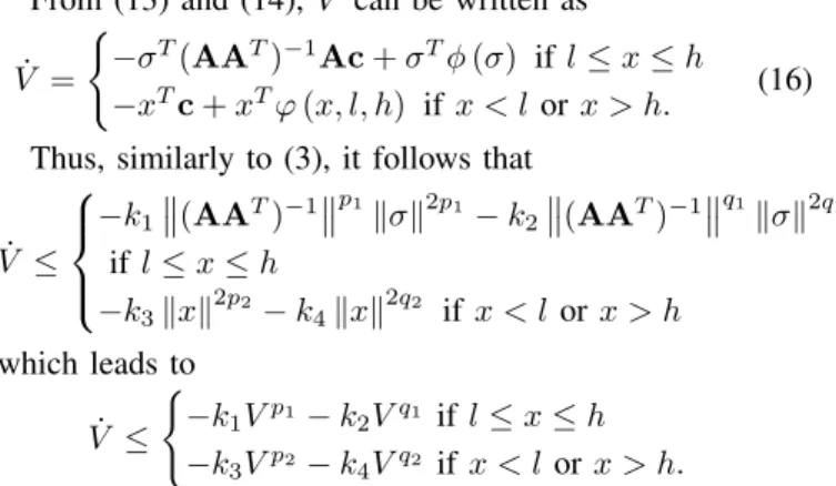
In Fig. 5, the utility grid behavior is shown. It can be seen that the real power is close to the PGmin which is set as 0

watts. 50 100 150 200 250 −15 −10 −5 0 5 10 15 Time (sec) Power(watt)

Utility Grid Power

Utility Grid Power Utility Grid Power Reference

Fig. 5. Utility grid power and utility grid power reference.

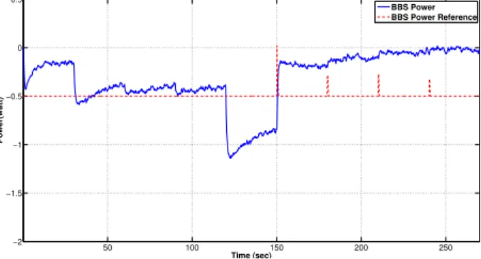
In Fig. 6, the WPS power and its reference is displayed. It can be noted that this module approaches to its reference all the time. Fig. 7 and Fig. 8 show how SPS and BBS modules attend to reach their power references even though a related controller for these modules has not been developed yet. BBS tracking error is higher than SPS, because the power contribution of this module depends on the state of charge of the batteries. 50 100 150 200 250 −25 −20 −15 −10 −5 0 5 10 15 Time (sec) Power(watt) WPS Power WPS Power WPS Power Reference

Fig. 6. Wind power and wind power reference.

50 100 150 200 250 −2 −1.5 −1 −0.5 0 0.5 Time (sec) Power(watt) SPS Power SPS Power SPS Power Reference

(7)

50 100 150 200 250 −2 −1.5 −1 −0.5 0 0.5 Time (sec) Power(watt) BBS Power BBS Power BBS Power Reference

Fig. 8. Battery power and battery power reference.

V. CONCLUSION

In this paper, a new dynamical system which solves linear programming is presented. Its main features are fixed convergence time and fixed parameter number despite the problem dimension. In the simulation results it is shown the independence from the initial conditions and the convergence time. Furthermore, the method structure can be extended from a small to a high dimension problem statement, without a convergence time alteration. The optimization algorithm is used to obtain the optimal solution for a Microgrid laboratory energy distribution problem. The algorithm gives the references to track for all the energy sources connected to the prototype, minimizing the consumed power from the utility grid. The presented results validate the optimization method for a real-time application. As future work, the proposed algorithm will be extend to solve other convex optimization problems.

REFERENCES

[1] I. B. Pyne, “Linear programming on an electronic analogue computer,”

American Institute of Electrical Engineers, Part I: Communication and Electronics, Transactions of the, vol. 75, no. 2, pp. 139–143, 1956. [2] S. K. Korovin and V. I. Utkin, “Using sliding modes in static

optimization and nonlinear programming,”Automatica, vol. 10, no. 5, pp. 525 – 532, 1974.

[3] S. V. Drakunov and V. Utkin, “Sliding mode control in dynamic systems,” International Journal of Control, vol. 55, pp. 1029–1037, 1992.

[4] L. Chua and G.-N. Lin, “Nonlinear programming without computa-tion,”IEEE Transactions on Circuits and Systems, vol. 31, no. 2, pp. 182–188, 1984.

[5] D. Tank and J. Hopfield, “Simple ’neural’ optimization networks: An A/D converter, signal decision circuit, and a linear programming circuit,”IEEE Transactions on Circuits and Systems, vol. 33, no. 5, pp. 533–541, 1986.

[6] R. W. Brockett, “Dynamical systems that sort lists, diagonalize matrices and solve linear programming problems,” inProc. 27th IEEE Conf. Decision and Control, 1988, pp. 799–803.

[7] M. P. Kennedy and L. O. Chua, “Neural networks for nonlinear programming,”IEEE Transactions on Circuits and Systems, vol. 35, no. 5, pp. 554–562, 1988.

[8] L. V. Ferreira, E. Kaszkurewicz, and A. Bhaya, “Convergence analysis of neural networks that solve linear programming problems,” inNeural Networks, 2002. IJCNN ’02. Proceedings of the 2002 International Joint Conference on, vol. 3, 2002, pp. 2476–2481.

[9] M. Forti, P. Nistri, and M. Quincampoix, “Generalized neural network for nonsmooth nonlinear programming problems,”IEEE Transactions on Circuits and Systems I: Regular Papers, vol. 51, no. 9, pp. 1741– 1754, 2004.

[10] Q. Liu and J. Wang, “A one-layer recurrent neural network with a discontinuous activation function for linear programming,”Neural Computation, vol. 20, no. 5, pp. 1366–1383, Nov. 2007.

[11] J. D. Sanchez-Torres, E. N. Sanchez, and A. G. Loukianov, “Recurrent neural networks with fixed time convergence for linear and quadratic programming,” inNeural Networks (IJCNN), The 2013 International Joint Conference on, 2013, pp. 1–5.

[12] F. A. Pazos and A. Bhaya, “Control Liapunov function design of neural networks that solve convex optimization and variational inequality problems,”Neurocomputing, vol. 72, no. 1618, pp. 3863 – 3872, 2009. [13] M. Glazos, S. Hui, and S. Zak, “Sliding modes in solving convex programming problems,”SIAM Journal on Control and Optimization, vol. 36, no. 2, pp. 680–697, 1998.

[14] G. Wilson, “Quadratic programming analogs,”IEEE Transactions on Circuits and Systems, vol. 33, no. 9, pp. 907–911, 1986.

[15] A. Rodriguez-Vazquez, R. Dominguez-Castro, A. Rueda, J. L. Huertas, and E. Sanchez-Sinencio, “Nonlinear switched capacitor ‘neural’ networks for optimization problems,”IEEE Transactions on Circuits and Systems, vol. 37, no. 3, pp. 384–398, 1990.

[16] J. Wang, “Analysis and design of a recurrent neural network for linear programming,”IEEE Transactions on Circuits and Systems I: Fundamental Theory and Applications, vol. 40, no. 9, pp. 613–618, 1993.

[17] A. Cichocki and R. Unbehauen,Neural networks for optimization and signal processing. J. Wiley, 1993.

[18] W. Karush, “Minima of functions of several variables with inequalities as side constraints,” Master’s thesis, Dept. of Mathematics, Univ. of Chicago, Chicago, Illinois., 1939.

[19] H. W. Kuhn and A. W. Tucker, “Nonlinear programming,” inProc. Second Berkeley Symp. on Math. Statist. and Prob. (Univ. of Calif. Press), 1951.

[20] C. M. Dorling and A. S. I. Zinober, “Two approaches to hyperplane design in multivariable variable structure control systems,”

International Journal of Control, vol. 44, no. 1, pp. 65–82, 1986. [21] V. Utkin, Sliding Modes in Control and Optimization. Springer

Verlag, 1992.

[22] E. Cruz-Zavala, J. Moreno, and L. Fridman, “Uniform second-order sliding mode observer for mechanical systems,” inVariable Structure Systems (VSS), 2010 11th International Workshop on, june 2010, pp. 14 –19.

[23] A. Polyakov, “Nonlinear feedback design for fixed-time stabilization of linear control systems,”IEEE Transactions on Automatic Control, vol. 57, no. 8, pp. 2106–2110, 2012.

[24] S. Chowdhury and P. Crossley, Microgrids and Active Distribution Networks, ser. IET renewable energy series, IET, Ed. Institution of Engineering and Technology, 2009.

[25] J. Patino, A. M´arquez, and J. Espinosa, “An economic MPC approach for a microgrid energy management system,” inIEEE PES Transmission & Distribution Conference and Exposition (T&D-LA), 2014.

[26] R. Aquino, M. Carvalho, O. Neto, M. M. S. Lira, G. de Almeida, and S. Tiburcio, “Recurrent neural networks solving a real large scale mid-term scheduling for power plants,” inNeural Networks (IJCNN), The 2010 International Joint Conference on, 2010, pp. 1–6. [27] L. J. Ricalde, E. Ordonez, M. Gamez, and E. N. Sanchez, “Design of

a smart grid management system with renewable energy generation,” in Computational Intelligence Applications In Smart Grid (CIASG), 2011 IEEE Symposium on, 2011, pp. 1–4.

[28] A. F. Filippov, Differential equations with discontinuous righthand sides, Mathematics and . its Applications (Soviet Series), Eds. Kluwer Academic Publishers Group, Dordrecht, 1988.