W&M ScholarWorks
W&M ScholarWorks
Undergraduate Honors Theses Theses, Dissertations, & Master Projects4-2020
Nonnegative Matrix Factorization Problem
Nonnegative Matrix Factorization Problem
Junda An
Follow this and additional works at: https://scholarworks.wm.edu/honorstheses
Part of the Algebra Commons, and the Other Applied Mathematics Commons Recommended Citation
Recommended Citation
An, Junda, "Nonnegative Matrix Factorization Problem" (2020). Undergraduate Honors Theses. Paper 1518.
https://scholarworks.wm.edu/honorstheses/1518
This Honors Thesis is brought to you for free and open access by the Theses, Dissertations, & Master Projects at W&M ScholarWorks. It has been accepted for inclusion in Undergraduate Honors Theses by an authorized administrator of W&M ScholarWorks. For more information, please contact [email protected].
c
2020 Junda An
NONNEGATIVE MATRIX FACTORIZATION PROBLEM Junda An, B.S.
College of William and Mary 2020
The Nonnegative Matrix Factorization (NMF) problem has been widely used to analyze high-dimensional nonnegative data and extract important features. In this paper, I review major concepts regarding NMF, some NMF algorithms and related problems including initialization strategies and near separable NMF. Fi-nally I will implement algorithms on generated and real data to compare their performances.
ACKNOWLEDGEMENTS
First of all, I would like to express my sincere gratitude to my advisor Professor Charles Johnson for his continuous support of my undergraduate study and research, and for his motivation, enthusiasm, and immense knowledge. His guidance helped me in all the time of research and writing of this thesis.
Besides my advisor, I would like to thank the rest of my thesis committee: Professor Gexin Yu and Professor Martin White, for their insightful comments and inspiring questions.
Last but not least, I would like to thank my parents: Dewen An and Huichun Zhou, for giving birth to me at the first place and supporting me throughout my life.
CHAPTER 1 INTRODUCTION
1.1
Problem Statement
The Nonnegative Matrix Factorization problem has been extensively studied since [Le Se] proposed simple and useful algorithms to approach this problem in 1999. After they published their work, there have been many algorithms at-tempting to solve this problem and several variants. Our goal is to state the NMF problem, explain algorithms we know, and introduce some further exten-sions of NMF.
The NMF is stated as follows. Given anm×nmatrixXand a positive integer r < min{m,n}, find nonnegative matricesW ∈R+m×r andH ∈Rr+×n to minimize the function f(W,H) = 12||X − W H||2
F. X is not equal to W H in most cases, but the
productW His called a nonnegative factorization ofX. So, strictly speaking, this problem should be phrased as Nonnegative Matrix Approximation problem, since factorization refers to an exact decomposition of the target matrix. How-ever, the NMF is so ubiquitous that it stands for an approximation problem by convention.
1.2
Background
In the context of NMF, the given matrix X contains original nonnegative data and each column is a m-dimensional data sample. W is a matrix of basis vec-tors, where each column is a basis vector. Columns ofW are not required to be
orthogonal to each other. His a weight matrix, in which each row is the gain of the corresponding basis vector. Therefore, X = W H can be geometrically inter-preted as every data points inX is contained in the cone generated by columns ofW,cone(W).
There are many challenging issues regarding the NMF. First, it is NP-hard [VA], which means it is very difficult to find an optimal solution. Unlike the unconstrained factorization problem which can be solved exactly with singu-lar value decomposition, it is hard to find the global minimum of the target function, f(W,H). Therefore, people have proposed many iterative algorithms that converge to stationary points. There exist many local minima due to the nonconvexity of f(W,H)in both W and H. Therefore, NMF is not only an NP-hard problem, but also a problem for which we may not get an exact answer. The extreme difficulty has led to many proposed algorithms that are not easily compared theoretically. One interesting observation is that f(W,H)is convex in eitherHorW. In other words, given a fixedH, we can efficiently find a unique solutionW that minimizes f(W,H)by using least square computation and forH given W. This observation is important, because it is used in one of the most efficient algorithms, Alternating Least Squares, to solve NMF. We discuss this in the following chapter.
The second challenge is that the NMF problem is ill-posed, because there does not exist a unique solution, even when the factorization is exact. For ex-ample, ifW H is a solution, we can also find a pair of W0 = W Dand H0 = D−1H so thatW0H0 = (W D)(D−1H) = W(DD−1)H = W H, whereDis a positive diagonal matrix. We can easily check thatW0 ∈ Rm×r
+ and H0 ∈ Rr+×n. Geometrically, if we
can find a different conic hull formed by columns of anotherW0, with a different weight matrix, which also contains all data points inX.
Despite such challenges, the NMF continues to be an area of much investiga-tion, because of a growing variety of important applications, like image feature extraction [Le Se2] [Gu] and text mining [Ga] [Di Li].
1.3
Preliminary
1.3.1
Notations
Rm×n set ofm×nreal matrices
Rm×n set ofm×nnonnegative real matrices
|| · || Frobenius norm
Xi: ithrow of matrix X
X:j jthcolumn of matrixX
X:S columns of matrixXindexed by the elements in setS
Xi:j element located at theithrow and the jthcolumn of matrixX
cone(X) cone generated by columns of matrixX
[X]+ projection of matrixXonto the nonnegative orthant
σ1(X) maximal singular value of matrix X
arg maxx f(x) value x that maximizes the value of the function f
1.3.2
Matrix Theory
Theorem 1.3.1. (Singular Value Decomposition [Jo Ho]) Every matrix X with rank k can be represented as X = Pk
i=1σiuivTi, where σ1 ≥ σ2 ≥ ... ≥ σk > 0 are positive
singular values ofXand{ui,vi}ki=1are corresponding left and right singular vector pairs
.
Theorem 1.3.2. (Eckart-Young-Mirsky Matrix Approximation Theorem [Go]) Given a matrixA ∈ Rn×m, the best rankr approximation to Ais the sum of firstrsummands
that isXr = P r
i=1σiuivTi =
Pr
i=1σiCi = UrΣrVrT, in whichXr is a rank-r approximation,
Ci = uivTi , columns ofUr ∈ Rm×r (resp. of Vr ∈ Rn×r) are the left (resp. right) singular
vectors, andΣris a diagonal matrix containing singular values on its diagonal.
1.4
Rank-one approximation
Lemma 1.4.1. (Perron-Frobenius Theorem [Jo Ho]) SupposeA∈Rn×nis nonnegative.
There is an eigenvalueρ(A)that is real and positive with left and right eigenvectors.
For any other eigenvalueλ,ρ(A)>|λ|.
SinceX is nonnegative,XXT
and XTX
are nonnegative. Therefore, there are nonnegative left and right singular vectors u1 and v1 associated with the first
singular value σ1. According to Theorem 1.3.2, σ1u1vT1 is the optimal rank-one
approximation of X. Since u1 and v1 are nonnegative, W H is the optimal
CHAPTER 2
EXISTING ALGORITHMS
In this chapter, I am going to describe existing algorithms from three main categories, which are multiplicative update methods, gradient descent meth-ods, and alternating least squares (ALS) methods. ALS was first introduced by [Pa, Ta] for the positive matrix factorization. However, this problem did not gain much attention until [Le, Se] reintroduced it as NMF and proposed multi-plicative update methods. This simple algorithm stimulated the wide research and applications of NMF not only in mathematics but also on image processing, text processing, bioinformatics, and etc. Another common practice to approach NP-hard problems is to use gradient descent. In each iteration, we need to cal-culate the gradient of our target function, f(W,H), choose a suitable step size, and update matrices by taking a step in the direction of the negative gradient. Later, HALS, an improved version of ALS was introduced, which will converge more efficiently.
All of the above algorithms can be fitted into a general framework to solve NMF:
(a) Initialize starting matricesW0and H0.
While do not satisfy stopping condition do: (b) FixHiand updateWi+1such that||X−WiHi||2
F ≥ ||X−W
i+1Hi||2
F.
(c) FixWi+1and updateHi+1such that||X−Wi+1Hi||2
F ≥ ||X−W
i+1Hi+1||2
F.
The efficiency of each algorithm depends on how many computations are needed in (b) and (c) and how many iterations are needed for the algorithm to
converge.
In the following sections, I will start by talking about multiplicative update method. Then, I will explain gradient descent and alternating least squares methods. In the last section, I will talk about singular value decomposition update method and why it fails.
2.1
Multiplicative Update
Algorithm 1:Multiplicative Update Method initializeW0andH0. i=0;
whiledo not satisfy stopping conditiondo updateWi+1= Wi◦ [Wi[HXi((HHi)i)TT]+] ;
updateHi+1= Hi◦ [(Wi+[(1W)Ti+W1)i+T1XH]i+] ; i=i+1
end
Note that◦and [.]
[.] denote the component-wise product and division. is a
sufficient small but positive number to prevent the denominator becoming zero. [Le Se] has shown that the Frobenius norm is non-increasing under the up-date rules, that is
||X−WiHi||2F ≥ ||X−Wi+1Hi||2F, ||X−Wi+1Hi||2F ≥ ||X−Wi+1Hi+1||2F.
[Le Se] also claimed that Algorithm 1 will converge to a local minimum, which was questioned by [Go, Zh] and [Li]. Moreover, when some entries inW and H become zero, those entries cannot be modified anymore and stay zero.
Therefore, [Be, Br] concludes that when Algorithm 1 converges to a limit point in the interior of the feasible region, the limit point is a stationary point, which, however, might be a saddle point. When Algorithm 1 converges to a limit point on the boundary of the feasible region, the stationary point cannot be deter-mined.
Even though Algorithm 1 often converges in practice, it is slow to converge, especially whenXis dense [Ha]. Since Algorithm 1 is a wildly used NMF algo-rithm, it is considered a baseline algorithm.
2.2
Projected Gradient Descent
Algorithm 2:Gradient Descent MethodinitializeW0andH0. i=0;
whiledo not satisfy stopping conditiondo updateWi+1= [Wi−Wi(WiHi−X)(Hi)T]+;
updateHi+1= [Hi−Hi(Wi+1)T(Wi+1Hi−X)]+; i=i+1
end
To minimize the objective function, f(W,H)with nonnegative constraint, we need to use gradient descent with a projection function, P(x) that maps x to the nearest feasible region. Here, we choose P(x) = [x]+. In order to minimize
f(W,H), we need to find the stationary point by calculating the gradient.
∂||X−W H||2
F
∂W =(W H−X)H
∂||X−W H||2
F
∂H =W
T
(W H−X)
LetW andH be step sizes. Then, we updateW andHby
Wnew =[W−W(W H−X)HT]+
Hnew = [H−HWT(W H−X)]+
The convergence of Algorithm 2 depends on the choice of the step size. A poor choice of the step size like setting it to be a fraction might lead Algorithm 2 converge to a factorization not far from the starting matrices. [Li], [Jo], and [Da] have found smart choices for the step size and proved the convergence of their algorithm.
Algorithm 3 is also sensitive to the starting matrices. [Li] indicated that if W0 and H0 are starting matrices such that||X −W0H0||2
F ≥ ||X||
2
F, very often after
the first iteration W1 = 0and H2 = 0, making the algorithm stop. Therefore, a careful choice of starting matrices are needed.
2.3
Alternating Least Squares
Algorithm 3:Alternating Least Squares Method initializeW0andH0. i=0;
whiledo not satisfy stopping conditiondo
(1) FixHiand solve forWi+1: Wi+1 =arg min
W≥0 12||X−W Hi||2F ;
(2) FixWi+1and solve forHi+1: Hi+1= arg minH≥0 12||X−Wi+1H||2F ;
i=i+1; end
As discussed in the first chapter, the NMF is not convex in both W and H, but it is convex in either ofW andW, when the other is fixed.
Based on this observation, NMF can be approached by iteratively solving a least squares problem with a nonnegative constraint. We consider (1) or (2) as a subproblem in Algorithm 3. Each subproblem can be decoupled into a collection of multiple nonnegative least squares problems. Take (2) as an example. We can solve (2) by solving each column ofHi+1from:
Hi:+j1 =minh≥0||X:j−Wi+1h||, (3)
where Hi:+j1 is the jth column of Hi+1 and X:j is the jth column of X.
Meth-ods in [La] and [Br] can be applied to solve the collection of nonnegative least squares problems. Algorithm 3 will converge to a local minimum, proved by [Gr, Sc] and [Li]. However, we need to solve m+ nnonnegative least squares problems in (1) and (2) per iteration, sinceW hasmrows and Hhasncolumns.
Hence, Algorithm 3 might be slower than Algorithm 1. Algorithm 4:Practical Alternating Least Squares Method
initializeW0andH0. i=0;
whiledo not satisfy stopping conditiondo FixH and solveW: W HHT = XHT ;
W = [W]+;
FixW and solveH: HTWTW = XTW ; H= [H]+;
i=i+1; end
[La] proposed Algorithm 4 to address the issue of the high cost of time in Algorithm 3. It uses a standard unconstrained least squares method in [Bj] to solve (1) and (2) by ignoring the nonnegative constraint and projects the answer to the nonnegative orthant. There is no proof that Algorithm 4 will converge to a local minimum, so it may generate a saddle point. Therefore, Algorith 4 sacrifices the convergence property for speed.
To preserve the convergence property and speed up the algorithm, [Ci] de-signed an algorithm called hierarchical alternating least squares (HALS). In stead of solving a whole matrix at a time, HALS find H or W by successively updating a column inWand a row inH. In a single step of updating a column-row pair, we fix all other variables and the problem is reduced to
min W:j,Hj:≥0 ||X−W H||2F = min W:j,Hj:≥0 ||(X−X k,j W:kHk:)−W:jHj:||2F = min W:j,Hj:≥0 ||X(j)−W:jHj:||2F, (4)
need to find the stationary point by calculating the gradient. ∂||X(j)−W:jHj:||2F ∂W:j = W:jHj:HTj:−X(j)HTj: =0 ∂||X(j)−W:jHj:||2F ∂Hj: = W:TjW:jHj:−W:TjX(j) =0
Then, updateW:j andHj: by
W:newj = [X(j)H T j:]+ Hj:HTj: Hnewj: = [W T :jX(j)]+ WT :jW:j
In practice, we may normalize the column vectorW:j and the row vectorHj:
to unit length vectors after each update. Therefore,W:newj = [X(j)HTj:]+and H
new j: =
[WT
:jX(j)]+. We get the final update rules by substituting X(j) = X−
P k,jW:kHk: = X−W H+W:jHj:. W:newj =[(XHT):j−W(HHT):j+W:jHj:HTj:]+ Hnewj: = [(WTX)j:−(W T W)j:H+W T :jW:jHj:]+
Algorithm 5:Hierarchical Alternating Least Squares Method initializeW0andH0. i=0. ;
whiledo not satisfy stopping conditiondo Ai =X(Hi)T ; Bi =Hi(Hi)T ; for j= 1,2, ...,rdo Wi+1 :j =[A i :j−W iBi :j+W i :jH i j:(H i)T j:]+; end Ci = Wi+1X; Di =(Wi+1)TWi+1; for j= 1,2, ...,rdo Hi+1 =[Cij:−Dij:H+(Wi+1)T :jW i+1 :j H i j:]+; end i=i+1; end
Note thatW:jand Hj: only affect each other. In one iteration, onlyrcolumns
inWandrrows inH. are updated Also note thatXHT andHHT does not change when we are updating columns in W. Therefore, we calculate XHT and HHT before we update columns in W. Similarly, WTX
and WTW
does not change when we are updating rows inH. Thus, we calculateWTXandWTW before we
update rows inH.
If we directly truncate negative elements to0, we may have some zero blocks which will stay zero and cannot update in every iteration. Therefore, the algo-rithm cannot converge in this case. To solve this problem, we use[]+ symbol, where [x]+ = max(,x)and is a sufficiently small but positive value. You can
CHAPTER 3
NEAR SEPARABLE NMF
3.1
Problem statement
While NMF is NP-hard, [Ar] proved that NMF can be solved in polynomial time under the separability assumption.X ∈Rm×n
isr-separableifX =W H, whereW ∈
Rm×r,H ∈Rr×nand columns ofW are a subset of columns ofX. Geometrically,X
isr-separable, if and only if all columns ofXreside in the conical hull generated by a subset ofrcolumns inX. Therefore, X = W Hcan be rewritten asX = X:SH,
where S denotes the subset of r columns of X, whose conical hull contains all columns of X. [Ar] refers to these columns as anchors or extreme rays. IfS is determined, thenHcan be easily calculated by solving a set of nonnegative least squares problems:
H:j = min h≥0
||X:j−X:Sh||2F, f or j=1,2, ...,n
Note thatHcan be expressed as[Ir, H0]P, whereIr ∈Rr×ridentity matrix,P∈ Rn×nis a permutation matrix, andH
0
∈Rr×(n−r). SinceHcan be easily found given
a fixedW, the problem can be reduced to findS which contains the anchors. In real applications our target matrix X will not have an exact NMF with a lower inner dimension, so X will not be perfectly r-separable. Therefore, we want to develop algorithms to find an NMF of anr-separable matrix with some noise. A matrixXisnoisy r-separableornear separable, if
where N ∈Rm×n
is a noise matrix with||N:i||2 ≤ for allifor some sufficiently
small. Geometrically, all columns ofXapproximately reside in the conical hull of its anchors. In the following section, two algorithms that are robust to noise are introduced.
3.2
Algorithms
There are two types of geometric approaches to solve the near-separable NMF. The first deals with convex hulls and the second deals with conical hulls. We will specifically discuss one representative algorithm for each approach in the following parts.
3.2.1
SPA
Lemma 3.2.1. IfX isr-separable andD∈Rn×n
is an invertible diagonal matrix,XD−1 is alsor-separable.
Proof. XD−1= X:SHD−1 = X:SDS−1:SDS:SHD−1 = (XD−1):SH
0
, whereH0 = DS:SHD−1 ∈
Rr×n.
Let Dbe a diagonal matrix, where Di:i = ||X:i||1. Then, XD−1 is separable by
Lemma 3.2.1. Then the columns of XD−1 is normalized, while the entries of every column of H0 sum to one. Then, every column in XD−1 can be as a data point. So, all points of XD−1 reside in the convex hull of r points in the set S. Then, the problem is reduce to finding the extreme points of a convex hull to
findS. [Gi] applies Successive Projection Algorithm (SPA) proposed by [Ar Sa] to find the extreme points.
Algorithm 6:Successive Projection Algorithm SetR1 = X,S1 = {}, andi= 1;
whileRi
, 0andi≤rdo
Solve for j: j= arg maxj||Ri:j||
2 2; Ri+1 =(I− R i :j(R i :j) T ||Ri :j||22 )Ri; Si+1 =Si∪ {j}; i=i+1; end
In the case of tie, the index jwhose corresponding column of the original matrixX with maximuml2norm will be selected. If there is
another tie, randomly select jamong those columns.
SPA works as follows: in the beginning, it lets the residual matrix be the target matrix. Then, it selects the point which has the greatest l2 norm in the
residual matrix, as it corresponds to an extreme vertex in the convex hull, which will be proved in the following part. Next, all data points are projected onto the orthogonal complement of the selected point. It repeats the process until r extreme points are selected. Note that after the first iteration, the residual matrix will typically have negative entries. However, it does not undermine the algorithm, since it does not set a nonnegative constraint to the residual matrix and it selects columns from the target matrix.
Why SPA can extract the extreme vertices is proved as follows [Gi]. Lemma 3.2.2. LetM =[W,0m×(r−k)]∈
Rm×r, whereW ∈Rm×kis full-rank andr >k≥ 0.
||Yh||22 <max
j
||W:j||22, ∀h∈Rr such thath,ei for all i
Proof. IfYh =0, then||Yh||2
2 =0. SinceWhas full rank,W:j ,0for all j. Therefore,
||W:j||22 >0= ||Yh||22.
Therefore, assume Yh = Pk
j=1hjW:j, wherehj , 0for at least one 1 ≤ j ≤ k.
Then, ||Yh||2F =|| k X j=1 hjW:j||22 < k X j=1 hj||W:j||22≤ max j ||W:j|| 2 2
The first inequality is strict because h , ei for all i and h has at least one
nonzero entryhj. The second inequality is due to our construction thatPki hi ≤
Pr
i hi ≤1.
Note that Lemma 3.2.2 implies that the column with the maximuml2 norm
in the matrixX = W Hwill always be a column inW.
Theorem 3.2.3. Let the matrix X = W H with every column normalized. Then SPA recovers the setS such thatX:S =W up to permutation.
Proof. Let us prove this theorem by induction.
Base step: Since W has full rank, Lemma 3.2.2 applies. Therefore, the first iteration of SPA extracts a column inW. Assume without loss of generality that the column extracted is W:j. Then, we can get the first residual matrix R1 =
(I− W:jW
T
:j
||W:j||22
Induction step: Assume that after k iterations the residual matrix is Rk =
[Wk,0m×k]
HwithWk full-rank. Then, the next iteration will extract a column that corresponds to one of the columns Wk
. The next residual matrix will become Rk+1 =[Wk+1,0m×(k+1)]whereWk+1 has full rank sinceWk
has full rank. Therefore, afterriterations, SPA will extract all columns ofWand the residual is zero.
Thus, SPA can extract extreme vertices in the target matrix in the noiseless case if these extreme vertices are linearly independent. [Gi] also shows that SPA is robust when noise is present in our target matrix. However, Theorem 3.2.3 is based on the assumption thatWhas full rank. If the assumption is not met, SPA will fail to recover more thanrank(W)columns fromW whenW is not full rank, even if X is noiseless. In order to overcome this drawback, [Gi2] developed Successive Nonnegative Projection Algorithm by modifying the update rule for the residual matrix. SNPA is more computationally expensive but more robust than SPA.
3.2.2
X
RAYXRAY identifies an anchor by completing selection and projection steps in an
it-eration.
In the projection step, all data points are projected onto the current cone by solving the nonnegative least squares problem,arg minH≥0||X−X:Si+1H||2
F and
compute a new residual matrix by R = X − X:Si+1H. Note that every residual columnR:k is orthogonal to one of faces of the current cone after the projection
In the selection step, a face of the current cone is selected by picking a resid-ual columnR:k. [Ku] observed and proved that for a given residual columnR:k
and any data X:j projected onto the current cone cone(X:Si), RT
:kX:j ≤ 0 if X:j is
inside the cone andRT
:kX:j >0ifX:j is outside the cone. Therefore, all points that
are exterior to the current cone are on one side of the hyperplaneRT
:kx>0, while
points contained in the cone are on the other side. The pointX:jthat maximizes
the inner product RT:kX:j
||X:j||1 is furthest from the hyperplane, so we select it as an an-chor to expand the current cone. [Ku] defines multiple approaches (rand, max, and dist) to select a face of the current cone. All of these approaches can find anchors in separable cases but behave differently in the presence of noise.
Algorithm 7:XRAY
SetR= X,Si ={}, andi=1; whileR, 0andi≤rdo
Selectkaccording to one of following criteria: rand :any randomksuch that||R:k||2;
max:solve fork: maxk||Rk||;
dist :solve fork: maxk||[RTkX]+||2 ;
Solve for j: j=arg maxj RT
:kX:j
||X:j||1
Si+1 =Si∪ {j};
Solve forH: H= arg minH≥0||X−X:Si+1H||2
F
R= X−X:Si+1H end
Although XRAY only takesr iterations to complete, it is not computationally
cheap because it has to solve the nonnegative least squares problem in the pro-jection step. Furthermore, even without the presence of noise, XRAY will fail to
inner product and one of these columns is a conic combination of the others. [Ku] did not give a rigorous analysis of XRAY in the near-separable case, which
CHAPTER 4 INITIALIZATION
As mentioned in chapter 1, NMF is NP-hard, so the best one can do is to use iterative methods to find local minima. Starting too far from a stationary point, too many iterations will be needed to converge. Therefore, good initialization strategies are needed to converge to a competitive stationary point and reduce convergence time.
4.1
The SVD
The singular value decomposition (SVD) is a standard tool to generate a lower-rank matrix decomposition when there are no constraints. According to Eckart-Young-Mirsky Matrix Approximation Theorem, the best rankr approximation toX is the sum of firstrsummands that isXr =P
r
i=1σiuivTi = P r
i=1σiCi =UrΣrVrT,
in whichXris a rank-r approximation,Ci = uivTi , columns ofUr ∈ Rm×r(resp. of
Vr ∈ Rn×r) are the left (resp. right) singular vectors, andΣr is a diagonal matrix
containing singular values on its diagonal. However, with the nonnegativity constraint, we can only guarantee thatC1is nonnegative by Lemma 1.4.1, while
for i > 1, Ci typically has negative entries. Therefore, Ur and ΣrVr cannot be
used directly as a starting point. There are two methods that have been used to modify the SVD to get a nonnegative approximation.
[Qi] proposed an algorithm called SVD-NMF which approximates X by |Ur|Σr|VrT|. It initializes W = |Ur|and H = Σr|VrT|. However, simply taking the
for error bounds and performance of this approach in the existing literature. [Bo] proposed a more widely used algorithm called the nonnegative double SVD (NNDSVD). It uses the SVD on the positive part ofCi. It further
decom-posesXras follows: Xr= r X i=1 σiCi =σ1C1+ r X i=2 σiCi =σ1C1+ r X i=2 σiCi+− r X i=2 σiCi− = σ1C1+ r X i=2 σiσ1(C+i)u1(C+i )v1(Ci+) T − r X i=2 σiσ2(C+i )u2(Ci+)v2(C+i) T r X i=2 −σiCi−,
in which σi(Ci+)is the ith largest singular value of C+i and ui(Ci+) and vi(Ci+)
are the ith left and right singular vectors of C+i. Note that [Bo] proved that rank(Ci+) ≤ 2, so Ci has at most two singular values. SinceC+i is nonnegative,
its rank-1 approximation is also nonnegative by the Perron-Frobenius theorem. NNDSVD approximates Xr by truncating the negative part. For the starting
matricesWandH, the first column (resp. row) ofW(resp. H) will beσ11/2u1(resp.
σ1/2
1 v
T
1) and theith column (resp. row) ofW(resp. H) will be(σiσ1(Ci+))
1/2u 1(Ci+) (resp. (σiσ1(C+i)) 1/2v 1(C+i ) T ).
Note that forrsufficiently large, the difference betweenXand its rank-r ini-tial approximation will grow as r grows, since more negative entries are trun-cated. This is a problem in both initialization strategies since it would make more sense that the approximation will be better as r grows, as in the uncon-strained rank-r approximation. [Sy] modified the initialization strategy to over-come this problem.
4.2
Clustering
[Di] showed that the K-means clustering on nonnegative data is equivalent to NMF. [Wi] directly applied the K-means clustering method proposed by [Ma] to initialize columns inW, taking the columns of X as data to be clustered and columns ofW as centroids. His initialized as the cluster indicator matrix (Hi,j =
1ifX:j belongs to theith cluster). Since the K-means clustering method is itself
iterative, the main drawback of this initialization strategy is its expensive cost.
4.3
SPA
As discussed in Chapter 3, SPA is an efficient and reproducible method to find extreme points in a convex hull in the separable case. However, without the sep-arability assumption, the extreme points may not present in the points in target matrix. Therefore, SPA cannot be directly used for the non-separable case. How-ever, it might provide a good starting point, since the key idea of SPA is to find points such that the geometrical hull formed by these points is as large as pos-sible. SPA gives a more structured starting point than the random initialization and is faster than SVD-based or clustering initializations. Even if SPA does not select best points, the NMF algorithm can still adjust the approximation. How-ever, SPA is sensitive to outliers. For example, if we have a perfect convex hull that contains all points except one outlier, SPA might select this outlier, since it wants to expand the hull.
CHAPTER 5
EXPERIMENTS AND CONCLUSION
5.1
Experiments
In this section, four NMF algorithms and three Initialization strategies are tested on the CBCL data set [CB] . CBCL data set contains 2429 greyscale19×19facial images. Therefore, X, the matrix obtained from this data set is a 361× 2429
nonnegative matrix, in which each column is a vetorized representation of an image.49basis images are used to approximateX, sor= 49.
The first experiment was conducted by running MU, CD, ALS, and HALS on X, with the same randomly initialized matrices twenty times. The average error was obtained by taking the average of each time. The second (third) ex-periment were conducted by running MU (HALS) with SVD, SPA, and random initializations.
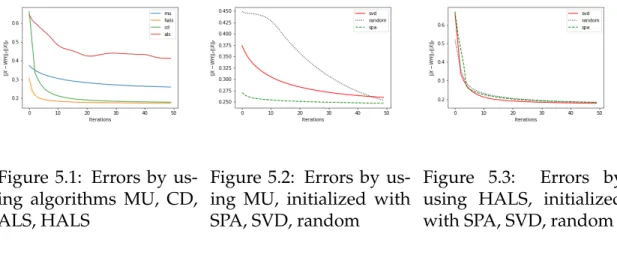
Figure 5.1: Errors by us-ing algorithms MU, CD, ALS, HALS
Figure 5.2: Errors by us-ing MU, initialized with SPA, SVD, random
Figure 5.3: Errors by using HALS, initialized with SPA, SVD, random
From Figure 5.1, we can observe:
• MU converges relatively slowly
• HALS converges the fastest and the error is the lowest
• The error of CD is comparable to HALS.
From Figure 5.2 and Figure 5.3, we can observe:
• For the MU algorithm, SPA will give the best starting matrices and con-verge the fastest.
• For the HALS algorithm, three initialization strategies are comparable and the SVD method is slightly better.
5.2
Conclusion
The NMF is a useful dimensionality reduction technique for nonnegative data, with wide applications in different disciplines. Due to its usefulness and ex-treme difficulty, the NMF has led to abundant research. Although there may not be an optimal solution for the general NMF, researchers have solved some extensions of the NMF that have some nice properties, like the nonnegative fac-torization of a separable matrix. With the greater computational capacity of current computers, more heuristic algorithms have emerged. Meanwhile, we believe more fundamental theories underlying this problem also need to be ex-plored and studied.
BIBLIOGRAPHY
[Te Pa] Paatero, Pentti and Unto Tapper. “Positive matrix factorization: A non-negative factor model with optimal utilization of error estimates of data values.” (1994).
[Le Se] Lee, Daniel Seung, Hyunjune. (2001). Algorithms for Non-negative Matrix Factorization. Adv. Neural Inform. Process. Syst.. 13.
[VA] Vavasis, Stephen. (2007). On the Complexity of Nonnegative Matrix Factorization. SIAM Journal on Optimization. 20. 10.1137/070709967.
[Le Se2] Lee, Daniel Seung, H.. (1999). Learning the parts of objects by nonnegative matrix factorization. Nature. 401.
[Gu] Guillamet, David Vitri`a, Jordi. (2002). Non-negative Matrix Factor-ization for Face Recognition. Topics in Artificial Intelligence. 35. 336-344. 10.1007/3-540-36079-4-29.
[Ga] Gaussier, Eric Goutte, Cyril. (2005). Relation between PLSA and NMF and implications. Proc. Annual Int. SIGIR Conf. Res. Develop. Inform. Re-trieval (SIGIR’05). 28. 601-602. 10.1145/1076034.1076148.
[Di Li] Ding, Chris Li, Tao Peng, Wei, 2008. ”On the equivalence between Non-negative Matrix Factorization and Probabilistic Latent Semantic Indexing,” Computational Statistics Data Analysis, Elsevier, vol. 52(8), pages 3913-3927, April.
[Li] Lin, Chih-Jen. (2007). On the Convergence of Multiplicative Update Al-gorithms for Nonnegative Matrix Factorization. Neural Networks, IEEE
Trans-actions on. 18. 1589 - 1596. 10.1109/TNN.2007.895831.
[Be, Br] Berry, Michael Browne, Murray Langville, Amy Pauca, V.Paul Plemmons, Robert. (2007). Algorithms and Applications for Approximate Non-negative Matrix Factorization. Computational Statistics Data Analysis. 52. 155-173. 10.1016/j.csda.2006.11.006.
[Ha] Han, Jian Han, Lixing NEUMANN, M Prasad, Upendra. (2009). On the rate of convergence of the image space reconstruction algorithm. Operators and Matrices. 3. 10.7153/oam-03-02.
[Jo] Johansson, Bj ¨orn Elfving, Tommy Kozlov, V. Censor, Yair Forss´en, Per-Erik Granlund, G ¨osta. (2006). The application of an oblique-projected Landwe-ber method to a model of supervised learning. Mathematical and Computer Modelling. 43. 892-909. 10.1016/j.mcm.2005.12.010.
[Da] Dai, Yu-Hong Fletcher, Roger. (2005). Projected Barzilai-Borwein meth-ods for large-scale box-constrained quadratic programming. Numerische Math-ematik. 100. 21-47. 10.1007/s00211-004-0569-y.
[La] Lawson, C. Hanson, Richard. (2020). Solving least squares problems prentice-hall.
[Br] Bro, Rasmus Jong, Sijmen. (1997). A Fast
Non-negativity-constrained Least Squares Algorithm. Journal of Chemometrics. 11. 393-401. 10.1002/(SICI)1099-128X(199709/10)11:53.0.CO;2-L.
[Li] Lin, Chih-Jen. (2007). Projected Gradient Methods for
Non-Negative Matrix Factorization. Neural computation. 19. 2756-79.
[Gr, Sc] Grippo, L.. (2000). On the convergence of the block nonlinear Gauss-Seidel method under convex constraints. Operations Research Letters. 26. 127-136. 10.1016/S0167-6377(99)00074-7.
[La] Albright, Russell Cox, James Duling, David Langville, Amy Meyer, Carl. (2014). Algorithms, initializations, and convergence for the nonnegative matrix factorization. Proc. 12th ACM SIGKDD Int. Conf. Knowl. Disc. Data Mining.
[Bj] Bj ¨orck, ke,. (1996). Numerical Methods for Least Squares Problems. SIAM Philadelphia. 10.1137/1.9781611971484.
[Ho] Ho, Ngoc-Diep. (2008). Nonnegative matrix factorization algorithms and applications. PhD thesis.
[Ar] Arora, Sanjeev Ge, Rong Kannan, Ravi Moitra, Ankur. (2016). puting a Nonnegative Matrix Factorization—Provably. SIAM Journal on Com-puting. 45. 1582-1611. 10.1137/130913869.
[Gi] Gillis, Nicolas Vavasis, Stephen. (2013). Fast and Robust Recursive Algorithms for Separable Nonnegative Matrix Factorization. IEEE transactions on pattern analysis and machine intelligence.
[Ar Sa] Bezerra, Saldanha Galv˜ao, Roberto Yoneyama, Takashi Chame, Henrique Visani, Valeria. (2001). The successive projections algorithm for vari-able selection in spectroscopic multicomponent analysis. Chemometrics and Intelligent Laboratory Systems. 57. 65-73. 10.1016/S0169-7439(01)00119-8.
[Ku] Kumar, Abhishek Sindhwani, Vikas Kambadur, Prabhanjan. (2012). Fast Conical Hull Algorithms for Near-separable Non-negative Matrix
Factor-ization.
[Go] Golub, G.H. Hoffman, Alan Stewart, G.W.. (1987). A generalization of the Eckart-Young-Mirsky matrix approximation theorem. Linear Algebra and its Applications. s 88–89. 317–327. 10.1016/0024-3795(87)90114-5.
[Qi] Qiao, Hanli. (2014). New SVD Based Initialization Strategy for Non-negative Matrix Factorization. Pattern Recognition Letters. 63. 10.1016/j.patrec.2015.05.019.
[Bo] Boutsidis, Christos Gallopoulos, Efstratios. (2008). Gallopoulos, E.: Svd based initialization: A head start for nonnegative matrix factorization. Pat-tern Recognition 41(4), 1362. PatPat-tern Recognition. 1350 – 1362. 1350-1362. 10.1016/j.patcog.2007.09.010. [Sy] Atif, Syed Qazi, Sameer Gillis, Nicolas. (2019). Improved SVD-based initialization for nonnegative matrix factorization using low-rank correction. Pattern Recognition Letters. 122. 10.1016/j.patrec.2019.02.018.
[Wi] Wild, Stefan Curry, James Dougherty, Anne. (2004). Improving non-negative matrix factorization through structured initialization. Pattern Recog-nition. 37. 2217-2232. 10.1016/j.patcog.2004.02.013.
[Ma] McQueen, J.. (1967). Some methods for classification and analysis of multivariate observations. Computer and Chemistry. 4. 257-272.
[Di] Ding, Chris He, Xiaofeng Simon, Horst Jin, Rong. (2005). On the Equivalence of Nonnegative Matrix Factorization and K-means- Spectral Clus-tering. Proceedings of the 2005 SIAM International Conference on Data Mining. 10.1137/1.9781611972757.70.
[Jo Ho] Horn, R. A. Johnson, C. R. (1990). Matrix Analysis. Cambridge University Press.
[CB] MIT CBCL facial database, http://cbcl.mit.edu/cbcl/software-datasets/FaceData2.html