Neural Networks for CollaborativeFiltering

(1)

Neural Networks for Collaborative

Filtering

Von der Fakult¨at f ¨ur Mathematik und Informatik

der Universit¨at Leipzig

angenommene

D I S S E R T A T I O N

zur Erlangung des akademischen Grades

D

OCTOR

R

ERUM

N

ATURALIUM

(Dr. rer. nat.)

im Fachgebiet Informatik

vorgelegt von

Diplom-Wirtschaftsmathematiker Josef Feigl

geboren am 29. Mai 1985 in K ¨othen (Anhalt)

Die Annahme der Dissertation wurde empfohlen von:

1. Prof. Dr. Martin Bogdan, Universit¨at Leipzig

2. Prof. Dr. Barbara Hammer, Universit¨at Bielefeld

Die Verleihung des akademischen Grades erfolgt mit Bestehen

der Verteidigung am 02. Juli 2020 mit dem Gesamtpr¨adikat

(2)

(3)

ACKNOWLEDGEMENT

First of all, I would like to express my sincere gratitude to my advisor Prof. Dr. Martin Bogdan for his valuable advice and guidance from the beginning of this thesis until the end.

I would like to thank my supervisors at the Otto Group, Dr. Sabrina Zeplin, Timo Duchrow and Christian Rammig, for finding a work arrange-ment that enabled me to complete this thesis. A special thanks goes to my colleagues, Dr. Benjamin Bossan, Dr. Andreas Lattner and Marian Tietz for lots of helpful advice and many fruitful discussions.

Last but not the least, I would like to thank my parents and my girlfriend who supported me in all those years and helped me tremendously to find time to work on this thesis.

(4)

(5)

ABSTRACT

Recommender systems are an integral part of almost all modern e-commerce companies. They contribute significantly to the overall customer satisfac-tion by helping the user discover new and relevant items, which conse-quently leads to higher sales and stronger customer retention. It is, there-fore, not surprising that large e-commerce shops like Amazon or streaming platforms like Netflix and Spotify even use multiple recommender systems to further increase user engagement.

Finding the most relevant items for each user is a difficult task that is critically dependent on the available user feedback information. However, most users typically interact with products only through noisy implicit feed-back, such as clicks or purchases, rather than providing explicit information about their preferences, such as product ratings. This usually makes large amounts of behavioural user data necessary to infer accurate user prefer-ences. One popular approach to make the most use of both forms of feed-back is called collaborative filtering. Here, the main idea is to compare indi-vidual user behaviour with the behaviour of all known users.

Although there are many different collaborative filtering techniques, ma-trix factorization models are among the most successful ones. In contrast, while neural networks are nowadays the state-of-the-art method for tasks such as image recognition or natural language processing, they are still not very popular for collaborative filtering tasks. Therefore, the main focus of this thesis is the derivation of multiple wide neural network architectures to mimic and extend matrix factorization models for various collaborative filtering problems and to gain insights into the connection between these models.

The basics of the proposed architecture are wide and shallow feedforward neural networks, which will be established for rating prediction tasks on ex-plicit feedback datasets. These networks consist of large input and output layers, which allow them to capture user and item representation similar to matrix factorization models. By deriving all weight updates and compar-ing the structure of both models, it is proven that a simplified version of

(6)

ditionally, various extensions are thoroughly evaluated. The new findings of this evaluation can also easily be transferred to other matrix factorization models.

This neural network architecture can be extended to be used for person-alized ranking tasks on implicit feedback datasets. For these problems, it is necessary to rank products according to individual preferences using only the provided implicit feedback. One of the most successful and influential approaches for personalized ranking tasks is Bayesian Personalized Rank-ing, which attempts to learn pairwise item rankings and can also be used in combination with matrix factorization models. It is shown, how the intro-duction of an additional ranking layer forces the network to learn pairwise item rankings. In addition, similarities between this novel neural network architecture and a matrix factorization model trained with Bayesian Per-sonalized Ranking are proven. To the best of our knowledge, this is the first time that these connections have been shown. The state-of-the-art perfor-mance of this network is demonstrated in a detailed evaluation.

The most comprehensive feedback datasets consist of a mixture of ex-plicit as well as imex-plicit feedback information. Here, the goal is to predict if a user will like an item, similar to rating prediction tasks, even if this user has never given any explicit feedback at all: a problem, that has not been covered by the collaborative filtering literature yet. The network to solve this task is composed out of two networks: one for the explicit and one for the implicit feedback. Additional item features are learned using the implicit feedback, which capture all information necessary to rank items. Afterwards, these features are used to improve the explicit feedback predic-tion. Both parts of this combined network have different optimization goals, are trained simultaneously and, therefore, influence each other. A detailed evaluation shows that this approach is helpful to improve the network’s overall predictive performance especially for ranking metrics.

(7)

Chapter 1

Introduction

In modern e-commerce shops, users can be overwhelmed by the number of available items to choose from. For example, Amazon.com is selling several million different products[63], Netflix.com has a total of more than 15 000 movies in their library[9]and Spotify.com has tens of millions songs avail-able [49]. However, most of these items are usually not sold, watched or listened to very often. Only a small percentage of these items account for most sales. This is often called Long Tail effect (see Figure1.1)[5]. It can, therefore, be very difficult for uninformed users to find relevant new items. Most of them are uninteresting, the very popular items are usually already known or even owned and interesting niche items are almost impossible to find on its own.

The main goal of most e-commerce shops is to sell as many items as pos-sible to their users. Limiting the vast item selection with personalized item recommendations can substantially increase the probability of a purchase. The difficult task of selecting the most appropriate items given the users individual preferences is done by recommender systems[84].

(12)

0 2000 4000 6000 8000

Movies

0 20000 40000 60000 80000 100000

Po

pu

la

rit

y

Figure 1.1: Long-Tail-Effect. Less than 2 000 movies from a total of about 17 700 movies account for about 75% of all views (blue). Most movies only have a low amount of viewers (orange). The plot is based on the Netflix Prize dataset and shows only the distribution for the top 8 000 movies. Popularity is measured as the total amount of viewers per movie.

1.1 I

MPACT OF

R

ECOMMENDER

S

YSTEMS

Recommender systems have shown to be able to significantly increase the number of sold items, the diversity of sold items and the user satisfaction in general[85].

Today, recommendations are used extensively. Analysis of user behaviour on Amazon.com, famous for their progressive use of recommendation sys-tem, have shown that about 30% of all page views are influenced by them

[99].

The immense importance of recommender systems at Netflix is obvious today as about 80% of all hours streamed are influenced by them. Their movie recommender is, therefore, producing a value of more than 1 billion dollar per year[34,100]. Even before becoming a video streaming platform, Netflix used recommender systems for their DVD and Blu-ray rental ser-vice. They reported that even an 10% increase in accuracy of their movie

(13)

1.2 Problem Description and Forms of Feedback

recommendation system would yield a significant increase in revenue. This lead to the launch of the famous Netflix Prize competition, in which Netflix awarded 1 million dollar to the first team to achieve the largest improve-ment compared to their recommender system at the time[9]. With the start of the Netflix Prize competition, so called rating prediction problems be-came highly popular.

1.2 P

ROBLEM

D

ESCRIPTION AND

F

ORMS OF

F

EEDBACK

For rating prediction problems, we are given a dataset with ratings assigned to items by users. The task here is to predict the rating a user would assign to an item, which he has not rated yet. In this case, we are given explicit ratings, which means that a user explicitly told us about his preferences. He can express his satisfaction about an item unmistakable by assigning high ratings for good items or low ratings for, in his opinion, bad items. This form of feedback is called explicit user feedback and datasets consisting of explicit feedback are called explicit feedback datasets[57]. Despite their popularity, it is rather uncommon that users give explicit feedback about their individual preferences and the datasets associated with this feedback are, therefore, rather rare or have to be created separately, which can be expensive and time consuming.

It is much more common to collect user information by observing online behaviour. For e-commerce websites, this involves, for example, tracking which products the user purchased or looked at, which songs he listened to, which links he clicked or which movies he watched. In all of these cases, we collect information about a user interaction with an item. Each of these snippets reveals valuable information about their preferences. This form of feedback is called implicit user feedback[74].Here, a user does not explicitly specify whether or how much he likes an item. We only know that he has interacted with it in some way. Implicit feedback is especially useful for so called personalized ranking problems. For these tasks, it is sufficient to

(14)

rank appropriate items and not necessary to predict their explicit ratings. A recommender system would have to create a ranked list of items for each user, in which the item with the highest probability to be interesting for a user would be at the top of the users’ individual list.

Usually, recommender systems deal with both types of feedback sepa-rately. However, a more comprehensive and realistic scenario is given when trying to make use of a mixture of both sources of feedback. This is impor-tant because most users may not assign a single rating to an article, but some nevertheless and a good recommender system should not miss any of this valuable information. It is especially interesting and close to the reality of modern e-commerce sites when information about most users is limited to implicit feedback. We are using the terms mixed user feedback for the mix-ture of both implicit and explicit user feedback and mixed feedback datasets for the associated datasets.

All of these feedback forms contain valuable information necessary to in-fer individual user prein-ferences. However, they also share similar problems. Due to their sparsity and noisiness, it is usually required to collect large amounts of user data to train valuable recommender systems. Collabora-tive filtering methods have proven to be especially successful when dealing with such datasets.

1.3 C

OLLABORATIVE

F

ILTERING

Recommender systems can solve rating prediction or personalized ranking problems in multiple ways. A common approach uses meta information about items, for example, its color, price or release date, to find different but similar items. In the same way, similar users can be identified by com-paring user-specific meta information like age or gender. Models using this approach are called content based, because they are analysing the content or meta information of items or users[78].

The most successful approach for the Netflix Prize competition[56],and a very popular approach in general, is to use one user’s individual pref-erences and compare them with the prefpref-erences of all other users. This

(15)

1.4 Neural Networks

approach is called collaborative filtering, first developed at the Xerox Palo Alto Research Center to filter large amounts of emails[32]. The underlying assumption here is that if two users like (or dislike) the same items, they might also share the same preferences about unknown items.

There is a vast collection of popular collaborative filtering methods. Many of them are based on matrix factorization or k-nearest neighborhood models

[92]. Neural networks, however, are usually not the first choice for collabo-rative filtering problems, regardless of the large advancements that has been made in their training and application during the last decade.

1.4 N

EURAL

N

ETWORKS

Many improvements were made in the training of neural networks in re-cent years. For example, dropout [43], a technique to improve regulariza-tion of deep neural networks, or Adam [104], a sophisticated updater to speed up training convergence. This lead to various neural network ar-chitectures achieving state-of-the-art performances for many difficult tasks. Convolutional neural networks are the dominating force for solving image recognition tasks [58], word embeddings learned by neural networks are very popular for natural language modeling[68],recurrent neural networks are used for speech recognition[36]and WaveNets, a variant of deep neural networks, are able to generate raw audio[75].

1.5 M

OTIVATION

The usage of neural networks for collaborative filtering problems is still rel-atively insignificant compared to the many successful approaches in these other mentioned domains. A popular exception to this case are Restricted Boltzmann Machines (RBM[90]). These generative stochastic artificial neu-ral networks have proven to achieve strong performances on collaborative filtering tasks, for example, in the Netflix Prize competition[56].

(16)

Other approaches focus on multi-layer networks, for example Autoen-coders, unsupervised neural networks used typically for dimensionality re-duction, to learn user and item representations, which can than further be used to find similar users or items[98]. Stacked deep neural networks have also been shown to achieve a remarkable performance on many collabora-tive filtering tasks[41].

However, these deep network architectures increase the complexity of such a recommender system significantly. Each layer adds multiple hyper-parameters, for example, the layer size or the choice of activation function, which need to be well tuned to achieve a good predictive performance. Ad-ditionally, each layer increases training time and, thus, requires more puting power. And yet, the achieved predictive performance of these com-plex networks is usually still comparable to well tuned matrix factorization models[41, 60]. This raises the question if all of this additional complexity is really necessary to achieve strong performances on collaborative filtering tasks with neural network architectures.

There is one shallow and wide network architecture that shares many connections with matrix factorization models, which can also be used to solve collaborative filtering problems. First links between these two models were explored during the Netflix Prize competition[29]and slightly later in

[102]. However, these neural networks were usually just mentioned briefly. To the best of our knowledge, we are also not aware of any literature dealing with this architecture in depth. Furthermore, their application is yet also limited to rating prediction problems on explicit feedback datasets.

This neural network architecture offers, regardless of being not very well-known, many advantages. Due to its similarity with matrix factorization models, it should offer at least the same good predictive performance for collaborative filtering problems. We can also easily extend and modify it by using components of modern state-of-the-art networks, such as new activa-tion funcactiva-tions or popular updaters, usually used for different tasks, which will hopefully improve its predictive performance even further. The modu-larity of neural networks also allows us to easily extend this architecture to

(17)

1.6 Thesis Outline

different domains such as personalized ranking tasks on implicit feedback datasets or rating prediction problems on mixed feedback datasets.

The main focus of this thesis is, therefore, the exploration of this neu-ral network architecture for various collaborative filtering tasks. This thesis will contribute to the understanding of this architecture in three major parts: We will (1) extend these neural networks to personalized ranking problems on implicit feedback datasets and rating prediction problems on mixed feed-back datasets, (2) prove similarities between the proposed architectures and matrix factorization models for implicit and explicit feedback datasets and (3) adopt and thoroughly evaluate current state-of-the-art methods of neu-ral networks to further improve the predictive performance of our proposed recommender system.

1.6 T

HESIS

O

UTLINE

This thesis is organized as follows:

Chapter 2

The main part of this chapter introduces the most important concepts of neural networks, starting with the basics of feedforward networks. This includes, for example, the notation of all weights in these net-works, which we will make heavy use of throughout the whole thesis, or the training using back-propagation and gradient descent. After-wards, we will also discuss more advanced topics such as the Adam optimizer or state-of-the-art activation functions. The last part of this chapter introduces recommender systems and collaborative filtering techniques in more detail. This includes, for example, the discussion of feedback properties or common problems recommender systems have to deal with.

Chapter 3

This chapter focuses on rating prediction problems. After a detailed problem definition, we will give a thorough introduction about matrix factorization models used to solve this problem. Afterwards, we will

(18)

introduce a neural network architecture suitable for this problem and show similarities with common matrix factorization models. Addition-ally, we will show how to extend the network and further improve its predictive performance. At the end of this chapter, we will thoroughly evaluate the models performance on several popular datasets used for rating prediction tasks.

Chapter 4

The main focus of this chapter is about personalized ranking problems. Here, we will extend the previously introduces neural network archi-tecture to implicit feedback datasets. We will prove similarities be-tween our model and a matrix factorization model trained using the popular Bayesian Personalized Ranking criterion. Various extensions to this network are evaluated at the end of this chapter in multiple ex-periments.

Chapter 5

In this chapter, we will combine both previously introduced architec-tures to solve collaborative filtering tasks for mixed feedback datasets. We will exploit implicit feedback information to improve the predictive performance of an explicit recommender system. Additionally, we will show how to use this model even for users that never gave any explicit feedback.

Chapter 6

In the last chapter of this thesis, we will summarize our findings and give an outlook on future research.

1.7 U

SE OF

P

ERSONAL

P

RONOUN

The personal pronoun ”we” is used throughout the whole thesis, although it represents the work of only one single author. The main reason for doing so is that all papers, this thesis is build on, were written using this style.

(19)

1.7 Use of Personal Pronoun

In addition, we believe that most readers will be familiar with this style of writing, which has become widespread in recent years.

(20)

(21)

Chapter 2

Basics

In this thesis, we will derive neural network architectures, similar to popu-lar matrix factorization models, to solve various collaborative filtering prob-lems. The proposed architecture is based on popular feed forward neural networks. It is, therefore, necessary to explain this neural network type in greater detail, which will be the main part of this chapter. Additionally, we will give an overview of common collaborative filtering techniques, data-sets and problems in the last part of this chapter.

2.1 F

EEDFORWARD

N

EURAL

N

ETWORKS

Feedforward neural networks are one of the most popular neural network architectures. Many steps were taken that led to the development of the first powerful neural feedforward networks. While it is difficult to narrow down the beginning of this development (see [96] for an extensive overview), an important milestone was made in 1943 by Warren S. McCulloch and Walter H. Pitts with the development of the first artificial neurons[66].Building on this foundation, Frank Rosenblatt published the first concept of the prede-cessor of modern feedforward networks in 1958: the (single-layer) percep-tron, which is a linear classifier for binary outcomes[88].

(22)

Although very popular model at the time, Marvin Minsky and Seymor Papert were able to show that this simple linear model was incapable of learning the well-known exclusive-or (XOR) function[69]. This was solved by organizing multiple perceptrons into layers, creating the much more powerful multi-layer perceptrons. It can be shown, that these networks are universal function approximator. Broadly speaking, they are able to approx-imate any non-linear function1[23,46].

Feedforward neural networks are structured in layers. Each layer con-sists of a number of neurons and each of these neurons is connected to the neurons of the subsequent layer. All information moves in only one direc-tion through the network. Starting at the input layer, all features are passed through multiple hidden layer until the output of the network is computed in the final layer. The input layer is providing the input features to the network, whereas the output layer coalesces all incoming information from the previous layer and produces the final predictions of the network. Most computations are performed in the cascade of hidden layers, which allow the network to approximate complex functions. One limitation of this ar-chitecture is that the connections between the units do not form cycles (as in recurrent neural networks)[11].

2.1.1 NOTATION

We now define the notations that refer to the weights in a feedworward neural network.

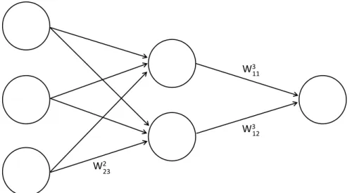
LetLlbe a single layer in the network. For example,L1refers to the input layer of the network. We defineWl_ij to be the single weight connecting the jthunit of layerLl−1with theithunit of layerLl.

(23)

2.1 Feedforward Neural Networks

Hidden Layer

Output Layer

Input Layer

12 W3 11 W3 23 W2

Figure 2.1: Feedforward neural network. Each layer is fully connected with the previous layer. The weight notations used throughout this thesis are exemplary shown for a few weights.

Following this notation, we define:

• Wl·uas the set of all outgoing weights from theuthunit of layer Ll−1to

all units of layer Ll

• W_il_· as the set of all incoming weights from layer Ll−1 connecting to theithunit of layer Ll

• Wlas the set of all weights connecting to thelthlayer

We will usually refer to these weights as weight matrices and use a bold let-ter to represent vectors and matrices. For example in Figure2.1, all weights connecting to the hidden layerL2are given by the weight matrixW2 ∈R3x2_.

2.1.2 FORWARD

PROPAGATION

Each neuron in the network is responsible for aggregating the incoming weights and inputs. This is done by computing a weighted sum of its

(24)

in-puts, adding a biasb and passing the result through the activation function fl :R→Rof layerl: zl_j =

∑

k W_jkl ·al_k−1+bl_j al_j = fl(zl_j). (2.1) We can also use a vectorized notation to describe the activation of a layerl:

zl =Wl·al−1+bl

al = fl(zl). (2.2)

Here, the inputafor a neuron is the activation of all neurons of the previous layer. We will use this vectorized notation for most parts of this thesis as it is shorter, more intuitive and, thus, more easily comprehensible.

The first inputa0is given by the input features presented to the network. Let thereforeX = (x1,x2,· · ·) be a set of input featuresx ∈ Rp for the net-work and y = (y1,y2,· · ·) be the corresponding targets, which are to be learned by the network. These very first input features can then be propa-gated forward through all layers of the network.

LetΩbe the set of all weights and parameters of the neural network. We can now define

NN(X,Ω) = aL

=yˆ (2.3)

as the result of the forward propagation of input X, which is done by ap-plying equations (2.2) on a0 = X. The activation of the output layer aL is synonymous with the output or predictions ˆyof the network.

2.1.3 BASIC

ACTIVATION

FUNCTIONS

The predictive performance of neural networks is heavily influenced by the choice of suitable activation functions.

(25)

In the original McCulloch&Pitts neurons, activation functions were only used to decide if a neuron should fire or not, which was inspired by bio-logical neural networks[11,66]. A step function, for example, the Heaviside step function or unit step functionHwith

H(x) :=    1, x≥0 0, else, (2.4)

was, therefore, used in these cases[11].2

While there is a vast selection of activation functions to choice from, only two are of major importance for the remaining part of this chapter:

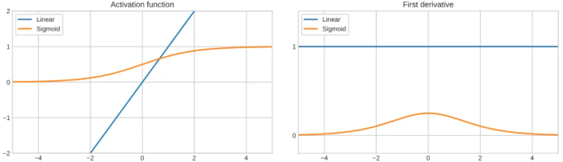
Identity

The identity or linear activation function is one of the most simple acti-vation functions as it only returns the given input:

f(x) = x (2.5)

f0(x) = 1 (2.6)

Sigmoid

This non-linear activation function is capped between 0 and 1 and often used if the desired output is to be interpreted as a probability. We will reserve the symbolσfor this activation function throughout this thesis:

σ(x) = 1

1+e−x. (2.7)

2_{A major drawback of this activation function is that its derivative is zero almost} every-where, which makes it unsuitable to be used in the training of neural networks. The reasons for this will be thoroughly explained in Subsection2.1.6.

(26)

−4 −2 0 2 4 −2 −1 0 1 2 Activation function Linear Sigmoid −4 −2 0 2 4 0 1 First derivative Linear Sigmoid

Figure 2.2: Basic activation functions. Identity and sigmoid activation functions (left) and their respective derivative (right).

Its derivative can be simplified to:

σ0(x) = ∂ ∂x(1+e −x₎−1 =−(1+e−x)−2·(−e−x) = 1 1+e−x · (1+e−x)−1 1+e−x = 1 1+e−x ·(1− 1 1+e−x) =σ(x)·(1−σ(x)) (2.8)

A visual representation of these basic activation functions and their deriva-tives can be found in Figure2.2. More advanced activation functions will be discussed in Subsection2.2.1.

2.1.4 LOSS

FUNCTIONS

Up to this point, we only know how to compute the output of a feedforward neural network, but not how to actually train the network to predict a target ygiven the inputX. For this, we need loss functions and a method to update the network weights to reduce the loss accordingly.

A loss function C defines the task, a neural network is required to opti-mize and allows measuring the quality of the learned representations. It quantifies the difference between the actual targets and the predictions of the network.

(27)

Two of the most common loss functions are the mean squared error (MSE) and the cross entropy loss (CE):

Mean squared error

The MSEloss function or quadratic loss function is defined as: CMSE(y, ˆy) := 1 n n

∑

i=1 (y_i−yˆ_i)2 = 1 n(y−yˆ) 2_. _(2.9)

This loss function is commonly used for regression problems. Due to the squaring of each term, it heavily penalizes outliers.

Cross entropy loss

The CE loss function is frequently used in neural networks for binary classification problems. It is defined as:

CCE(y, ˆy) := 1 n n

∑

i=1 y_i·ln ˆy_i+ (1−y_i)·ln(1−yˆ_i) =y·lnaL+ (1−y)·ln(1−aL). (2.10) For this loss function, the predictions ˆyhave to be probabilities of the real binary target classy[11].

There are many other loss functions, for example, the hinge loss function, which is used most notably in the training of Support Vector Machines (SV M) [21]. However, they are not of major importance for this thesis and will, therefore, not be discussed any further.

2.1.5 GRADIENT

DESCENT

Gradient descent is a classic first-order iterative function minimization algo-rithm originally invented 1847 by Louis Augustin Cauchy[18].The general idea is to calculate the gradient at any given point and take steps in the op-posite direction, which is also the direction of the steepest descent. The

(28)

pri-mary goal of the neural network training is to optimize the network weights Ωin such a way, that the previously defined loss functionCis minimized:

arg min

Ω C

(y, ˆy) (2.11)

The general update rule to find the weight updates for each weight is then given by

Ω ←Ω−λ ∂

∂ΩC(y, ˆy), (2.12)

where the parameter λ denotes the learning rate. This parameter

deter-mines the rate of approaching the minimum and is usually set to a small positive value. With each iteration of this algorithm, we are slowly mini-mizing our defined loss function.

The classic gradient descent method has many disadvantages. First of all, it is critically dependent on the choice of a suitable learning rate. Large learning rates may speed up training convergence but can also result in missing the (local) minimum and, therefore, decrease the predictive per-formance of the model. Very small learning rates, on the other hand, can increase the training time substantially [86]. Additionally, finding a local minimum of a function can only be guaranteed under certain conditions, for example, strong convexity of the function to be minimized[16]. Further-more, the gradient descent method can get stuck in local minima or con-verge only very slowly in some ill conditioned areas of the cost function[12,

13].

Despite all these problems, it is a simple and computationally fast method. It needs no second-derivative and works reasonably well even for very large datasets. Furthermore, some of these downsides can be alleviated with suit-able modifications (see also the upcoming Section2.2.3).

2.1.5.1 STOCHASTICGRADIENT DESCENT

One variation of gradient descent that became highly popular and basically the standard method for training (deep) neural network with many parame-ters is stochastic gradient decent[52,87].Instead of computing the gradients

(29)

for all samples, we now only select one random sampleifrom the training set to update the weightsΩ:

Ω←Ω−λ ∂

∂ΩC(yi, ˆyi). (2.13)

Each step is now very cheap, but the direction of the gradient from just one random sample might not be the best direction to reach the minimum. To mitigate this problem, a batch approach is usually more suitable. In this case, we are splitting the training dataset into random batches of psamples and update the weights after processing each batch[14]:

Ω←Ω−λ p p

∑

i=1 ∂ ∂ΩC(yi, ˆyi). (2.14)

This stochastic mini-batch approach for the training of neural networks has been found advantageous in many studies and leads to a significant speed-up of computation time[62].

Now, to be able to use (stochastic) gradient descent to train a neural net-work, all we need to know is how to find the gradients for all network weights efficiently.

2.1.6 BACKPROPAGATION

Computing gradients for all weights in almost any neural network is nowa-days usually done by using back-propagation. The roots of this method can be traced back until the early 1970s[51,96],but became popular in 1988 with a famous paper by David E. Rumelhart, Geoffrey E. Hinton and Ronald J. Williams[89]. The general idea of this algorithm is to compute the error between the output of the network ˆy and target y and back-propagate it through all layers of the network.

To formalize this process, we begin by defining the error of the output layerL:

δL = ∂

∂aLC· f

(30)

We can simplify this term significantly for both of our common loss func-tions.

For the mean squared error cost function, we use

∂

∂aLCMSE =a

L₋_y _(2.16)

to get

δL = (aL−y)· f0(zL). (2.17)

This can be simplified even further by using an identity activation function f in the last layer, which then yields:

δL =aL−y (2.18)

We will now repeat this process for the cross entropy cost function and a sigmoid activation functionσin the last layer:

δL = ∂ ∂aLCCE· f 0₍_zL₎ _(2.19) Using ∂ ∂aLCCE =y·lna L_{+ (}₁₋_y₎_·_ln₍₁₋_aL₎ =− y aL + 1−y 1−aL = a L ₋_y aL₍₁₋_aL₎ (2.20)

and (see Equation (2.8))

σ0(zL) = σ(zL)(1−σ(zL))

=aL(1−aL) (2.21)

finally yields

(31)

2.2 Advanced Neural Network Techniques

To summarize, whether we use the mean squared error cost function in com-bination with an identity activation function in the output layer or the cross entropy cost function in combination with a sigmoid activation function in the output layer, in both cases the error in the last layer is simply given by the difference between the output of the networkaL and the target y. We will make use of this result in the upcoming chapters of this thesis.

The error of the output layerδL can now be back-propagated through the

preceding layers. For all layersl = L−1,L−2, . . . , 2, we get[89]:

δl =Wl+1δl+1· f0(zl). (2.23)

Now that we have computed the error for all layers, we can compute the gradient for the loss functionCaccording to

∂ ∂Wl_jk C =al_k−1δl_j (2.24) and ∂ ∂bl_j C =δl_j. (2.25)

Using these gradients, we can apply (stochastic) gradient descent and itera-tively modify the weights of the net to minimize our defined loss function.

2.2 A

DVANCED

N

EURAL

N

ETWORK

T

ECHNIQUES

In the previous section, we explained how to train a neural network and make predictions for regression and classification problems. In this chapter, we will discuss how to improve its predictive performance and speed up the training time.

2.2.1 ADVANCED

ACTIVATION

FUNCTIONS

The search for optimal activation functions is still ongoing and a lot of re-search has been dedicated to this task in recent years. This has, for example,

(32)

lead to the use and further development of very popular rectified linear functions. We will now discuss some of the most commonly used activation functions that will also be used in the upcoming chapters of this thesis:

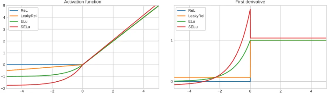
Rectified linear

With the rise of deep neural networks, rectified linear units (ReLUs) became highly popular[71]:

f(x) =max(0,x) (2.26) f0(x) =    1, ifx >0 0, otherwise (2.27)

Apart from being cheap to compute, it was shown, that this function is helpful to speed up training of deep convolutional neural networks for image recognition [58],help to learn sparse representations and avoid the vanishing gradient problem[31].

One problem might arise once a large part of all ReLUs of a network output only zeros. These neurons are then likely stuck in this state and are no longer helpful in discriminating the input. This is called dying ReLU problem, which can impact the predictive performance of the network[65].

Leaky rectified linear

Leaky rectified units (LeakyReLUs) are very similar to basicReLUs, but allow the output of small values for negative values ofx[65]:

f(x) =    x, ifx >0 x γ, otherwise (2.28) f0(x) =    1, ifx >0 1 γ, otherwise (2.29)

The parameterγis usually set to 100. Allowing small values on the

(33)

2.2 Advanced Neural Network Techniques −4 −2 0 2 4 −2 −1 0 1 2 3 4 5 Activation function ReL LeakyRel ELu SELu −4 −2 0 2 4 0 1 First derivative ReL LeakyRel ELu SELu

Figure 2.3: Advanced activation functions. We used the parametersγ =10 for the

LeakyReLfunction andλ=1,α=1 for theELfunctions.

dyingReLUproblem. These units were shown to improve convergence and predictive performance for deep neural network acoustic models

[65].

(Scaled) exponential linear

Exponential linear units (ELUs) differ from ReLUs only for negative values of x. The possibility of generating negative outputs in the pro-posed way proved to be advantageous in shortening the training time of deep neural networks and at the same time preventing the dying ReLU problem[20]. f(x) = λ    x, ifx >0 α(ex−1), otherwise (2.30) f0(x) = λ    1, if x>0 f(x) +α, otherwise (2.31)

The basic ELU version uses the parameter λ = 1 and α > 0. Using

the parameters λ ≈ 1.0507 and α ≈ 1.6732 yields the so-called scaled

exponential units (SELUs), which are able to ensure that activations with zero mean and unit variance will keep this property when being propagated through the network. This is often called a self-normalizing property[54].

(34)

A visual representation of these activation functions along with their deriva-tives can be found in Figure2.3.

2.2.2 REGULARIZATION

Modern neural networks often have multiple thousands or even millions of weights. For example, one of the state-of-the-art networks for image recog-nition tasks, a deep residual network with 152 layers has about 60 million parameters[39,109].With that many parameters, these networks need some kind of regularization to prevent them from overfitting the noise in the train-ing data. We will discuss four popular forms of regularization to prevent overfitting: L1- and L2 regularization, dropout and max-norm regulariza-tion.

2.2.2.1 L1-AND L2REGULARIZATION

L1- and L2 regularization are one of the most popular and longest known forms of regularization. Due to their wide usage in many fields, they are known under many different names. L2 regularization was originally intro-duced by Tikhonov in 1977 to solve ill-posed problems [105] and is, there-fore, also called Tikhonov regularization. Using L2 regularization to regu-larize least squares regression models yields so called ridge regression mod-els[44]and in the context of neural networks, it is often referred to as weight decay[35].Least squares regression models usingL1 regularization are also called Lasso (least absolute shrinkage and selection operator)[103]. Despite their various names and wide usage, the basic idea is always the same: to limit the growth of the model weights by shrinking them towards zero.

Applying any of these two regularization forms is usually done by adding a penalty termPto the unregularized loss functionC0:

(35)

TheL2 penalty is defined as the sum of the the squared magnitudes of the weightsW:

PL2(W) =δ2·

∑

w∈W

w2. (2.33)

Here, δ2 is the regularization parameter for the L2 regularization, which determines the strength of the regularization. This penalty term pushes all weights by a certain relative amount, depending on the weight, towards zero. Thus, it heavily penalizes large peaky weights, as these get decreased the most. The impact on small weight is relatively minor. However, the learned representations will usually be diffuse small numbers, which lack easy interpretability.

The L1 penalty term is defined as

PL1(W) =δ1·

∑

w∈W

|w|. (2.34)

Instead of pushing the weights by a certain relative value towards zero, we are now reducing the weights by an absolute valueδ1. This will, therefore, impact small weights stronger than large weights. Using this regularization will lead to sparse weight vectors with only few large weights. This makes it an effective tool for feature selection[73].

It is also possible to combine both penalties. The linear combination of L1 andL2 regularization is called elastic net regularization[111].

2.2.2.2 MAX-NORM REGULARIZATION

Max-norm regularization was originally introduced for matrix factoriza-tion models, but became also quite popular for neural networks [43, 101].

It works by enforcing an absolute upper bound on the magnitude of the weightsW:

||W||p ≤c. (2.35)

In this thesis, we only use p=2 as recommended in[43]. The upper bound cis usually in the range of[1, 4].

(36)

Its effectiveness as a form of regularization has a certain similarity with the L1- and L2 regularization methods. Max-norm regularization also at-tempts to limit the growth of the weights, but instead of shrinking them, it defines an upper bound. One of the appealing properties of this penalty is that the weights of the network cannot explode, even when the learning rate of the optimizer is set too high.

2.2.2.3 DROPOUT

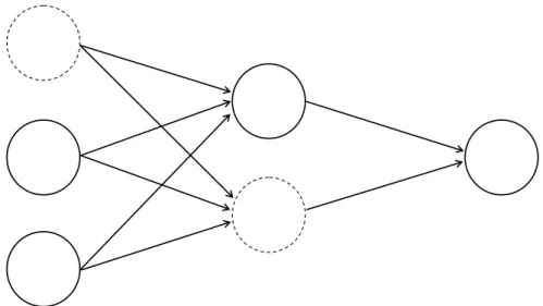
Dropout is possibly the most popular form of regularization for deep neural networks and used in many, if not all, state-of-the-art neural network archi-tectures for image recognition tasks[20,39].Its simple and effective general idea is to randomly ignore (drop out) a certain percentage of all neurons of a layer at each iteration (see Figure2.4). Therefore, we are basically sampling different sub-networks from the full neural netwotk at each training itera-tion. One natural explanation for its regularizing effect is that every neuron has to learn more robust features, since it cannot rely on the incoming

neu-Hidden Layer

Output Layer

Input Layer

Figure 2.4: Dropout. The first unit of the input layer and the second unit of the hid-den layer are dropped out (dotted lines), which means that their output is set to zero.

(37)

rons [43]. It is, therefore, quite different compared to the other discussed forms of regularization.

2.2.3 PARAMETER

UPDATES

In Section2.1.5, we have already explained how to use (stochastic) gradient descent to update all parameters of the neural network:

Ω ←Ω−λ ∂

∂ΩC(y, ˆy) (2.36)

We can define the parameter weight update∆W(t)and the gradientG(t)at training iterationtas

G(t) = ∂

∂ΩC(y, ˆy) (2.37)

∆W(t) =−λG(t) (2.38)

using the learning rateλ. It was also mentioned that one downside of this

method was its slow convergence. In this subsection, we explain three pop-ular ways to improve convergence and speed up training time: Momentum, RMSProp and Adam.

2.2.3.1 MOMENTUM

The most simple method of these three additions is Momentum. Its basic idea is to build up velocity whenever the gradient of the previous time step points in the same direction as the current gradient [79]. This is done by integrating updates of previous iterations:

∆W(t) = ρ∆W(t−1)−λG(t). (2.39)

We denote ρ as the momentum parameter. A common choice for this

pa-rameter is ρ = 0.9. Taking previous updates into account helps to smooth

out and avoid diverging oscillations, which enables the model to be trained in less iterations without losing predictive performance[11].

(38)

2.2.3.2 RMSPROP

While Momentum improves the convergence of the basic SGD method, it is still far from optimal. One major factor for the slow convergence speed is the global usage of a single learning rate parameter for all weight updates equally. One way to mitigate this problem is to use per-dimension learning rates, for example, by using a single adaptive learning rate for each weight. One of these adaptive learning rate methods is called Root Mean Square Propagation (RMSProp), which was applied with much success in practice

[94].

Here, we are dividing the gradient G(t) by the root of an exponential moving averageE(t)of the squared gradient:

E(t) = αE(t−1) + (1−α)G(t)2 (2.40)

∆W(t) = −ηp G(t)

E(t)2₊_γ (2.41)

Here, the parameter 0 < α <1 denotes the decay rate. The damping factor γis added to stabilize the denominator[104].

The biggest advantage over SGD and Momentum is that by deriving the per-dimension learning rates automatically, we are now less dependent on an optimal choice of the global learning rate η. One disadvantage of this

method is that the exponential moving averages of the past gradients have to be stored additionally.

2.2.3.3 ADAM

Another, more sophisticated, adaptive learning rate method is the Adaptive Moment Estimation method (Adam) [53]. It is an extension of RMSProp, which additional to the exponential moving average of past squared

(39)

gra-2.2 Advanced Neural Network Techniques

dients E(t), introduces an exponential moving average of past gradients similar to Momentum:

E(t) = β1E(t−1) + (1−β1)G(t)2 (2.42) M(t) = β2M(t−1) + (1−β2)G(t) (2.43) Theβ1andβ2parameters are initialized with values from the range of[0, 1], but usually close to 1. These two moment estimates are initialized with ze-ros and are biased towards zero, especially during the first iteration. They are, therefore, called biased moment estimators. The bias-corrected estima-tors are given by:

ˆ E(t) = E(t) 1−β1 (2.44) ˆ M(t) = M(t) 1−β2 (2.45)

Now, the parameter weight updates are given by: ∆W(t) = −η ˆ M(t) q ˆ E(t) +γ (2.46)

It was shown, that this methods also works especially well with sparse or noisy gradients[53].Most of our derived models throughout this thesis will use this optimizer.

2.2.4 I

MPLEMENTATION

FRAMEWORKS

All of the previously explained networks and network modifications can nowadays be implemented using open source libraries for numerical com-putation like TensorFlow[1]or PyTorch[77]. These frameworks are heavily optimized, highly customizable and allow to fully leverage the GPU, which usually speeds up model training significantly. For the proposed neural net-works derived later in this thesis, one training epoch using a Nvidia RTX 2060 was about 5−10 times faster than just using the CPU (6 cores).

(40)

All proposed neural networks in this thesis were implemented using Py-Torch 0.4.1. Whenever we refer to weight decay, the Adam or SGD opti-mizer, dropout or max-norm regularization, we make use of the default Py-Torch implementations. All networks can, of course, also be implemented in TensorFlow or comparable frameworks.

2.2.5 HYPERPARAMETER

OPTIMIZATION

Neural networks consist of many different hyperparameter. We usually have to choose, for example, the number of units per layer, select good ac-tivation functions, select an optimizer with appropriate learning rate or de-cide, which regularization method to use. Many of these choices are crucial for overall model performance, but finding good values can be time con-suming and computationally expensive. This hyperparameter optimization is usually done by grid-search or random-search algorithms[10].

In this thesis, the hyperparameter search was done in two steps. At first, an initial set of decent parameters was found by manual search. Afterwards, we used a local search algorithm to further optimize these parameters. This local search algorithm randomly selects a parameters and increases or de-creases it by about 10%. If this direction improves the current best score, the search continues this way, but not more than three times. Afterwards, it continues with the next parameter. This process is stopped after a fixed amount of iterations.

2.3 R

ECOMMENDER

S

YSTEMS

Recommender systems are information filtering technologies designed to provide suggestions for items of interest to a user [85]. Here, these items can, for example, be movies to watch, products to buy, songs to listen to, books to read or celebrities to follow.

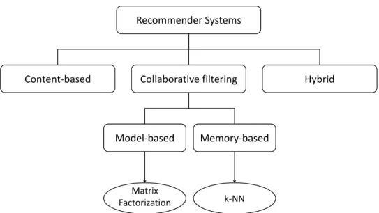
Recommender systems can roughly be distinguished into three main cat-egories: content-based, collaborative filtering-based or hybrid[17].

(41)

2.3 Recommender Systems

Content-based

Content-based recommendation systems use the metadata of users or items and the respective ratings associated with them to create new rec-ommendations. For example, a simple recommender system for books could use the author of the book as the only feature to create new sug-gestions. It would most likely only suggest new books from authors a user has already bought and liked in the past[17].

Collaborative filtering

Collaborative Filtering is essentially about predicting user preferences based on the preferences of other users [92]. Recommender systems based on collaborative filtering methods try to use a users’ past behav-ior to model the similarity between users (user-based collaborative fil-tering) or between items (item-based collaborative filfil-tering). The main idea is that similar users share similar interests and, therefore, also like similar items.

Hybrid

Hybrid recommender systems try to combine the two already men-tioned recommender classes, for example, by introducing additional content based features of an item into a collaborative filtering approach or by combining independently created content-based and collabora-tive filtering-based predictions into one ensemble model[2].

The main focus of this thesis is about the use of neural networks for col-laborative filtering systems. We will, therefore, use the remaining parts of this section to further define and explain collaborative filtering methods. Additionally, we will give details about popular collaborative filtering data-sets, which will be used throughout this thesis to evaluate all derived mod-els.

2.3.1 C

OLLABORATIVE

FILTERING

Collaborative filtering methods are among the most used techniques for rec-ommender systems. Amazon.com [63], Netflix.com [34] and Spotify [49],

(42)

Recommender Systems

Content-based Collaborative filtering Hybrid

Model-based Memory-based

Matrix

Factorization k-NN

Figure 2.5: Recommender Systems Overview. Matrix factorization andk-NN mod-els are given as examples of the above techniques. There are, of course, many more relevant models.

three multi-million dollar companies, all of which are well-known for their extensive use of recommendation systems, apply these methods in some way or another for their various recommendation systems.

Collaborative filtering methods can be further distinguished in two main groups: memory-based or model-based algorithms (see Figure2.5)[92].

Memory-based algorithms require all user, item and rating information to be stored in memory, which is then used for computing similarities be-tween users or items. There is a vast selection of similarity measures to choose from. For example, a very simple similarity measure could be the number of items two users have in common: the higher, the more similar they are. More sophisticated measures include Pearson correlation or co-sine similarity[2]. Afterwards, these similarities can further be used to find the nearest (most similar) neighbors of a user or an item (neighborhood-based algorithm). A common choice for selecting the k most similar users or items in these cases is thek-nearest neighbors algorithm (k-NN)[92].

The easy interpretability of memory-based algorithms is one of their great-est advantages. However, finding the perfect neighborhood can be

(43)

compu-2.3 Recommender Systems

tationally expensive as all users or items have to be compared against each other. Additionally, it can be difficult to compute accurate similarities be-tween users, who have rated only few or niche items, which applies to many sparse datasets.

Model-based collaborative filtering algorithms try to build a model repre-senting user behaviour, which is afterwards used to predict ratings or pref-erences. One popular variant of this approach are matrix factorization mod-els, which represent each user and item as a vector of factors and thus trans-forming them to the same latent factor space. Matrix factorization models for collaborative filtering tasks are one of the main themes of this thesis. We will, therefore, discuss them in much greater detail in the upcoming Chap-ter3.

2.3.2 C

OMMON

PROBLEMS

There are several typical problems all recommender systems, using either content-based or collaborative filtering approaches, have to deal with: cold start, sparsity, scalability and skewness.

Cold start

Recommender systems are trying to learn user preferences based on past behaviour. New users typically have no relevant behaviour his-tory and have never assigned any ratings to items. Since there is al-most no information about these users available, it is very difficult to find similar users or model their future behaviour. This is called the new user cold start problem and it is especially problematic for collab-orative filtering algorithms. Here, content based approaches (as used in hybrid recommender systems) can help to fill the gap for new users by relying on available user meta information, such as age or gender

[95].Of course, the same problem applies to new items, too.

Sparsity

For many datasets used in collaborative filtering, the number of users and items is very high. However, most users assign ratings only to a

(44)

few selected items. In this context, the ratio between all missing rat-ings and all available ratrat-ings is usually referred to as sparsity, which is typically very high for collaborative filtering datasets. It is, there-fore, necessary for recommender systems to make accurate predictions based on only a small number of relevant samples[2].

Scalability

Recommendation engines for large e-commerce companies often have to deal with millions of users and hundreds of thousands of items. Memory efficient algorithms and architectures are necessary to com-pute retime recommendations in those large-scale scenarios. As al-ready mentioned above, this can be especially problematic for memory-based collaborative filtering approaches, as the computational costs for computing pairwise similarities gets expensive very quickly[93].

Skewness

We have already talked about the fact that, as a general rule, only a very small percentage of all possible ratings are available. In addition, most of these reviews are assigned to the same items or by the same users. Some users are, therefore, responsible for a rather large percentage of all available assigned ratings, whereas most users have only rated very few items. The same holds true for all items. Popular items account for the vast majority of all assigned ratings, whereas niche items have only very few ratings. This problem is also called the Long Tail problem of recommender systems, since the item-popularity-distribution exhibits a strong positive skew (see also Figure1.1in the introduction)[3].

This is a selection of the most important problems. Other typical prob-lems, like the preservation of privacy[67],play no major part in this thesis.

2.3.3 FEEDBACK

PROPERTIES

To solve these mentioned problems and learn relevant user preferences, an effective recommender system has to extract as much information as possi-ble from all availapossi-ble sources of user feedback.

(45)

One of the most studied forms of feedback is explicit feedback. Here, a user assigned a rating to an item and, thus, explicitly informed us about his preferences. These ratings are usually unmistakably clear and easy to interpret: low ratings are assigned to unsatisfactory items and high ratings belong to good items. These ratings can often be chosen from a range of integers, for example [1, 5], or just binary {0, 1}. In most cases, however, it is relatively rare that users give explicit feedback at all. Easily available explicit feedback datasets are, therefore, rather scarce or have to be created especially for the task needed, which can be rather costly and time consum-ing.

Most of the time, users are just visiting a website or a store passively. Here, their preferences can only be learned from implicit feedback. Clicking on links, purchasing products, listening to a song or watching videos are typical examples where feedback is only given implicitly. With each click on an item, we have learned something about the user. Thus, instead of explicitly telling us about their preferences, we can only infer it by tracking their behaviour. Additionally, we can also easily convert explicit feedback to implicit feedback because each explicitly rated item is also an item with which the user has interacted.

Given this overview, it is rather obvious that the availability of explicit feedback is usually very low. Implicit feedback, however, is available in abundance[50]. While their vast availability is the main advantage of im-plicit feedback, it comes with many disadvantages. Imim-plicit feedback can only capture positive user preferences, which means that it is difficult to identify items a user does not like[47]. The reason for this is that if a user does not click on an item, it can have a number of meanings. He is either not interested, was simply not aware of the item or preferred another one. Whereas for explicit feedback, which usually provides rating scales, a user can accurately express his satisfaction with an item, whether is it positive or negative.

Implicit feedback is basically created while passively tracking the user. It is, therefore, inherently noisy. Misclicks on an item or link can happen much more easily than explicitly assigning a wrong rating. For example,

(46)

the playback of a song does not necessarily mean that the user likes it, he might simply not even be listening at all at this moment. Explicit feedback is noisy as well (as is every user feedback) but in general more accurate than implicit feedback as it usually takes more steps to give a wrong rating than to simply misclick. However, user preferences change over time and the assignment of ratings can be influenced by several factors like the rating scale, item ordering or the time taken to assign a rating[4,50].

2.3.4 COLLABORATIVE

FILTERING

DATASETS

2.3.4.1 NETFLIXPRIZE COMPETITION

The Netflix Prize competition was an important milestone in the develop-ment of recommender systems, especially for collaborative filtering meth-ods. During this competition, the research of recommender systems using only explicit feedback became very popular. In this thesis, we will also build on many ideas developed during this competition and additionally also use the Netflix Prize dataset for evaluating models. Therefore, it is worth to discuss this famous competition in a bit more detail.

The Netflix Prize competition ran over the course of three years from Oc-tober 2nd, 2006 until September 18, 2009 and more than 20 000 teams from 150 countries participated in it. The goal of this competition was to improve Netflix own recommender, Cinematch, by at least 10% (in terms of decreas-ing the root mean squared error).

A grand prize of 1 000 000 dollar was award to the first team able to achieve this goal. At the end, the competition was won by the team Bel-lKor’s Pragmatic Chaos. Their final ensemble model combined more than 100 single models and achieved a RMSE of 0.8567 besting Netflix own rec-ommender by 10.06%[56].The second placed team, The Ensemble, achieved the same improvement but submitted their result 20 min after the winning team (see Figure 2.6). A sequel competition was planned but ultimately cancelled in 2010 due to privacy concerns[72].

While many different machine learning models were used to solve this competition, matrix factorization models were especially successful.

(47)

Figure 2.6: Netflix Prize Leaderboard. The winning team submitted their result 20 minutes earlier than the second placed team. The final scores of all teams in the top 10 were achieved by blending multiple diverse models.

2.3.4.2 OTHER POPULAR DATASETS

We will use three benchmark datasets to evaluate our neural network archi-tectures:

Netflix Prize

This dataset was used in the Netflix Prize competition, which was al-ready mentioned above. With more than 100 million ratings, it is the largest dataset used throughout this thesis. Additionally, it is highly sparse and skewed with some very active users assigning ratings to more than 10 000 movies, but also with many users with less than 16 rated movies. A subset of this dataset, the probe set with 1 408 395 rat-ings, will be used as a validation set [9, 28]. All ratings are integers in the range of[1, 5].

MovieLens 1M

The MovieLens 1M dataset consists of about 1 million movie ratings made by about 6 000 users for about 4 000 movies [37]. Therefore, it is much smaller and slightly less sparse than the Netflix Prize dataset, but also commonly used in the evaluation of recommender systems. All ratings are integers in the same range as for the Netflix Prize dataset.

(48)

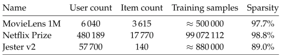
Table 2.1: Dataset statistics

Name User count Item count Sample count Sparsity MovieLens 1M 6 040 3 900 1 000 209 95.7% Netflix Prize 480 189 17 770 100 480 507 98.8%

Jester v2 59 132 150 1 700 000 80.8%

Jester

The Jester v2 dataset originates from an online joke recommending sys-tem. It consists of about 1 700 000 ratings made by about 57 000 users for 150 jokes [33]. The most interesting property of this dataset is the relatively low count of different items. The ratings are continuous be-tween−10 and 10.

A summary of the most important statistics of all datasets can be found in Table2.1.

(49)

Chapter 3

A Neural Network Architecture for

Explicit Feedback Datasets

In this chapter, we will derive two models for solving collaborative filtering problems on explicit feedback datasets. The first model will be matrix fac-torization model. We will show how to train this model and, additionally, introduce biases and common regularization methods for an improved pre-dictive performance. This model will be a strong baseline model, which will be heavily referred to in the upcoming chapters. The second model will be a neural network. At this point in the chapter, we will transition to the main theme of this thesis: neural network architectures for collaborative filtering problems. As a first step, we will show how to design a neural network to solve collaborative filtering problems on explicit feedback datasets.

The main result of this chapter will prove similarities between the pro-posed neural network model and the previously introduced matrix factor-ization model. Starting with a basic version of this neural network, we will extend it continuously by using state-of-the-art extensions of current neu-ral network models. At the end of this chapter, we will carefully evaluate several modifications of our proposed architecture.

(50)

3.1 D

EFINITION OF

E

XPLICIT

F

EEDBACK

D

ATASETS

We have already discussed general properties of explicit user feedback in Section2.3.3. We will now introduce a more formal view of explicit feedback datasets. Suppose we have a set of usersU ={1, . . . ,N} and a set of items I = {1, . . . ,M} with N,M ∈ N. For most typical problems, the user count N and the item count M are usually quite large. For example, the dataset used in the Netflix Prize competition consists of N = 480 189 users and M =17 770 items.

In explicit feedback datasets Sexpl, each useru ∈ Uexplicitly assigns rat-ingsr ∈ Rto itemsi∈ I. These ratings are usually binary valuesR={0, 1}, taken from a fixed set of integer values, for example R = {1, 2, 3, 4, 5}, or come from a continuous range of values, for example R = [−10, 10]. Each single sample of this dataset can, therefore, be defined as a triple (u, i, r). We use the notationrui ∈ Rfor the rating given to itemiby user u.

The explicit feedback datasetSexpl is, therefore, defined as:

Sexpl :={(u, i, r) | u∈ U,i ∈ I,r∈ R}. (3.1) For all explicit feedback datasets used in this thesis, we assume that each user rates an item at most once. This is also the case for all datasets we are working with throughout this thesis.

Explicit feedback datasets can be visualized by a table with three columns (see Table3.1).

3.2 M

ATRIX

F

ACTORIZATION FOR

E

XPLICIT

F

EEDBACK

D

ATASETS

In this section, we will show how to apply matrix factorization to collabo-rative filtering problems for explicit feedback datasets. To standardise the notation with the upcoming chapters, we will use the letter T to define a training dataset created from a feedback dataset S. For our case now, we

(51)

3.2 Matrix Factorization for Explicit Feedback Datasets

User Item Rating

1 2 1

1 3 5

2 1 2

2 4 4

3 4 1

Table 3.1: Explicit feedback datasets. An explicit feedback dataset with ratings from the range of[1, 5]. User 1 has rated two items. User 2 has assigned his highest rating to item 4. Each user rates an item at most once.

can simply setT=Sexpl, as we will use every sample fromSexplto train our model.

We have introduced explicit feedback datasets in Section 3.1 as a table with three columns. Another popular way to represent it is as a sparse ma-trixT ∈RN×M_{. Here, each row represents a user and each column an item.}

The entries of this matrix are given by the ratingsrui. This matrix is usually

very sparse as most entries are missing (see Figure3.1).

User Item Rating

1 1 1 1 2 3 2 3 4 3 1 5 3 3 4 1 2 4 5 4 Item User

Target Matrix

Explicit Feedback Dataset

Figure 3.1: Explicit Target Matrix. Each row of the explicit feedback dataset can be converted to a single entry in the sparse target matrix. This matrix has the same number of rows as there are distinct users and as many columns as there are items.

(52)

3.2.1 GENERAL

APPROACH

The basic idea behind matrix factorization is to decompose the target ma-trix T into multiple smaller low-rank matrices. One example of a well-known matrix factorization technique is called Singular Value Decompo-sition (SVD), which decomposes the target matrix into two o