Using Metrics Suites to Improve the Measurement of Privacy in Graphs

1

Using Metrics Suites to Improve the

Measurement of Privacy in Graphs

Yuchen Zhao and Isabel Wagner,

Senior Member, IEEE

Abstract—Social graphs are widely used in research (e.g., epidemiology) and business (e.g., recommender systems). However, sharing these graphs poses privacy risks because they contain sensitive information about individuals. Graph anonymization techniques aim to protect individual users in a graph, while graph de-anonymization aims to re-identify users. The effectiveness of anonymization and de-anonymization algorithms is usually evaluated with privacy metrics. However, it is unclear how strong existing privacy metrics are when they are used in graph privacy. In this paper, we study 26 privacy metrics for graph anonymization and

de-anonymization and evaluate their strength in terms of three criteria:monotonicityindicates whether the metric indicates lower

privacy for stronger adversaries; for within-scenario comparisons,evennessindicates whether metric values are spread evenly; and for

between-scenario comparisons,shared value rangeindicates whether metrics use a consistent value range across scenarios. Our

extensive experiments indicate that no single metric fulfills all three criteria perfectly. We therefore use methods from multi-criteria decision analysis to aggregate multiple metrics in a metrics suite, and we show that these metrics suites improve monotonicity compared to the best individual metric. This important result enables more monotonic, and thus more accurate, evaluations of new graph anonymization and de-anonymization algorithms.

Index Terms—graph anonymization, graph de-anonymization, privacy, privacy metrics, monotonicity, metrics suites

F

1 I

The usage of Internet-based communications systems such as email or social networks leaves traces that can be collected and stored in graph form. In these graphs, nodes represent users and edges represent relationships between users. Many graph data sets have already been published for scientific or commercial use [16], [17]. Graph data can help us understand social networks [15] and improve rec-ommendations [19], but can also harm user privacy because of sensitive information revealed by relationships.

To protect privacy, graphs can be anonymized by remov-ing node identifiers and by changremov-ing the graph structure. As a result, the nodes in the anonymized graph cannot easily be mapped to their original identifiers if the adversary does not possess additional knowledge. However, a common assumption is that adversaries know about an auxiliary graph with similar structure as well as the correct mapping for a small number of nodes. Finding new methods for anonymization and de-anonymization is an active research area [9], and researchers usually use privacy metrics to evaluate the effectiveness of their new methods.

The most commonly used metric in graph privacy is

the adversary’s success rate, which gives the percentage of

correctly re-identified nodes [10], [23], [27]. However, even though we show in this paper that the adversary’s success rate is indeed a good metric in many scenarios, it has two important shortcomings: First, it does not reveal much detail about the privacy of individual nodes because it measures

• Y. Zhao is with the School of Electronics and Computer Science, Univer-sity of Southampton, Southampton, SO17 1BJ, United Kingdom. • I. Wagner (corresponding author) is with the Cyber Security Centre, De

Montfort University, Leicester, LE1 9BH, United Kingdom. E-mail: [email protected], [email protected] Manuscript received MM DD, YYYY.

privacy on a per-graph level. Second, its common definition favors de-anonymization algorithms that primarily rely on local, instead of global, graph properties.

To find a better metric for graph privacy, we analyze privacy metrics proposed in other fields [36] in terms of three criteria: monotonicity, evenness, and shared value range [42]. Monotonicity requires that privacy metrics in-dicate lower privacy as the adversary’s strength increases. Evenness requires that the metric values are spread evenly over their value range, which improves within-scenario comparisons. Shared value range requires that metrics use a common value range even when they are applied to different datasets, anonymization, or de-anonymization al-gorithms. This improves between-scenario comparisons.

In this paper, we make the following contributions in the area of privacy measurement:

• We propose a framework for the evaluation of pri-vacy metrics for graph pripri-vacy based on our previous methodology [34], [42]. In contrast to the previous work, we tailor the method to graph privacy by using de-anonymization algorithms to model the adver-sary, defining adversary strength levels, and adding an anonymization step to the definition of user data.

• We conduct extensive experiments to analyze the

strength of 26 privacy metrics using 11 graph datasets, 11 anonymization algorithms, and 6 de-anonymization algorithms and find that no single metric excels in all three criteria.

• We find that several popular metrics are not mono-tonic in graph privacy, including entropy and the anonymity set size, and give a detailed analysis why this is the case. This finding is in contrast to results for other domains, such as vehicular network DOI: 10.1109/TDSC.2020.2980271 https://ieeexplore.ieee.org/document/9035391

(c) 2020 IEEE. Translations and content mining are permitted for academic research only. Personal use is also permitted, but republication/redistribution requires IEEE permission. See http://www.ieee.org/publications_standards/publications/rights/index.html for more information.

privacy [35].

• To the best of our knowledge, we are the first to use methods from multi-criteria decision analysis to integrate several metrics into a metrics suite. We evaluate four concrete metrics suites, synthesized using the Weighted Product Model, and show that our metrics suites have higher monotonicity than the best individual metric.

Our findings are important because our synthesis of metrics suites shows a convenient way how the strengths of multiple privacy metrics can be combined to improve the overall measurement of privacy.

2 B

2.1 Graph Anonymization and De-anonymization Structural graph de-anonymization algorithms and corre-sponding anonymization algorithms have been an active research area since the mid-2000s [2], when it was dis-covered that simply removing identifiers from nodes is not sufficient to prevent node re-identification. Since then, many anonymization and de-anonymization algorithms have been proposed [9].

In this paper, we use existing algorithms and implemen-tations [4], [5], [10], [39] to evaluate the strength of privacy metrics for graph anonymization and de-anonymization. We give more detail about the algorithms we used in Sec-tions 3.2 and 3.3.

2.2 Privacy Metrics for Graph Privacy

The most commonly used privacy metrics in graph anonymization and de-anonymization are the number of re-identified nodes [22] and the adversary’s success rate [10], [23], [27]. These metrics quantify privacy as the actual privacy breach that an adversary causes.

In the wider privacy research area, other classes of pri-vacy metrics have been proposed [36], for example measur-ing the adversary’s uncertainty, information gain, or error. For example, information-theoretic metrics such as entropy quantify privacy as the uncertainty that the adversary faces when re-identifying nodes. These metrics have shown good strength in other fields such as vehicular networks [42], but it is unknown whether they are suitable for graph privacy. In this paper, we examine the suitability and strength of a wide range of privacy metrics in graph privacy.

De-anonymizability quantification focuses on quantify-ing structural properties of graph pairs, such as the edge difference, to study the maximum number of nodes that could be de-anonymized, given only structural graph in-formation for a graph and a partially overlapping auxiliary graph [8], [24]. However, de-anonymizability quantification does not consider the interplay between anonymization and de-anonymization algorithms and has limited applicability in concrete practical scenarios due to its focus on theoretical limits for abstract graph models [9].

2.3 Utility Metrics for Graph Privacy

There is a trade-off between the privacy achieved by graph anonymization algorithms and the utility of the anonymized

graph. Utility is often measured according to how well the anonymized graph preserves the characteristics of the original graph, such as node degrees and path lengths [10]. In this paper, we focus on the quality of privacy metrics, and thus utility and utility measures are complementary to our study: How much utility a graph anonymization algorithm provides, or how this utility is measured, is independent of how its privacy properties are measured. We note that utility measures may be evaluated with similar methods as ours, but consider this to be out of scope for the current paper.

2.4 Criteria for Privacy Metrics

Several authors have proposed criteria that good privacy metrics should fulfill. For example, metrics should show the adversary’s chances of success [1], show the level of privacy and the potential for privacy violations [3], measure the amount of resources needed by the adversary [30], and integrate measurements for different aspects of privacy [28]. These criteria focus on properties that are desirable specifically in privacy measurement, such as consideration of the adversary. However, they do not focus on essential properties for measurement in general, such as consistency. In addition, these criteria do not allow to judge whether a privacy metric can discern differences in privacy levels between different users in a scenario, or between different scenarios.

To overcome these shortcomings, we use three criteria that we have proposed in prior work: monotonicity, even-ness, and shared value range. Taken together, these three criteria allow to select privacy metrics that result in consis-tent measurements, and from among those, to select privacy metrics that support the intended type of evaluation. 2.4.1 Monotonicity

Monotonicity indicates the consistency of measurement by requiring that higher amounts of privacy in a scenario are reflected in higher privacy levels. We have previously proposed to evaluate the monotonicity of privacy metrics with respect to the adversary, i.e. that they should show lower privacy levels for stronger adversaries [34], [42]. For example, we expect that, with increasing adversary strength, the values of the adversary’s success rate (as a lower-better metric) decrease, and that the values of entropy (as a higher-better metric) increase.

Monotonicity is a key property of privacy metrics be-cause a non-monotonic metric can make privacy-enhancing technologies, such as anonymization algorithms, appear stronger than they actually are. For example, non-monotonic metrics may indicate the same privacy level for strong and weak adversaries, or for strong and weak PETs. If these weak PETs are then deployed in practice, the use of non-monotonic metrics can lead to real-world privacy violations. We use the algorithm originally proposed in [34] to compute monotonicity scores for a privacy metricM. The algorithm uses two statistical tests (t-test and rank-sum test) to compare the mean values of the privacy metric for each pair of adjacent adversary strengths in a scenarioc, where a scenario is given by the combination of anonymizer, de-anonymizer and graph. For each statistical test, if the test indicates significance (p < 0.05) as well as a change in

the expected direction, the algorithm increases the metrics’ monotonicity score by 1. If the test indicates a change in the wrong direction, the algorithm subtracts 1 from the monotonicity score. If the changes in metric values change direction, e.g. increasing for one pair and decreasing for the next, the monotonicity score is reduced by 2 because such a peak may indicate the same privacy levels for both strong and weak adversaries and is thus undesirable. A metric’s final monotonicity score is the average of the scores for the two statistical tests, normalized to[0,1].

We formalize the notion of monotonicity specifically for graph privacy in Section 3.5.

2.4.2 Evenness and Shared Value Range

In addition to monotonicity, evenness and shared value range are desirable criteria for good privacy metrics, es-pecially if the metrics will be used for within-scenario comparisons and between-scenario comparisons [42].

Within-scenario comparisons compare the privacy levels of different nodes within the same graph. Ideally, the values of metrics for within-scenario comparisons should be spread evenly over the entire value range (evennessE). We compute the evenness of a metric’s value range based on the Cram´er-von Mises criterion, which measures the goodness of fit be-tween the uniform distributionF(xic)and the normalized metric valuesxic for all adversary strengths in a scenario

c. We normalize the Cram´er-von Mises criterion by the number of metric values n to offset the influence of the number of samples. E= 1 n( 1 12n+ n X i=1 [2i−1 2n −F(xic)] 2₎ (1)

Between-scenario comparisons compare privacy levels be-tween different graphs, and ideal metrics use the same value range regardless of the graph’s characteristics (shared value

rangeR). We formalize this notion by computing the portion

of the global value range for each metric that is used when the metric is applied to a specific graph.

R= max(xc)−min(xc)

max(x)−min(x) (2)

3 M

We evaluate the strength of privacy metrics for social graphs in terms of monotonicity, evenness, and shared value range. In this section, we explain our methodology, which we have adapted from our prior work [34], [42], [43]. Our method follows six steps, as illustrated in Figure 1:

1) Import an existing graph data set (Section 3.1) 2) Anonymize the input graph with different

anonymization algorithms (Section 3.2)

3) Subset the input graph to create an auxiliary graph and define seed mappings as prior information given to the adversary (Section 3.3)

4) Apply different de-anonymization algorithms to the anonymized graphs, controlling the adversary’s strength using the amount of prior information given to the adversary (Section 3.3)

5) Compute the values of privacy metrics based on the output of the de-anonymizer (Section 3.4)

6) Analyze the strength of each privacy metric accord-ing to the criteria of monotonicity (Sections 2.4.1 and 3.5), evenness, and shared value range (Section 2.4.2)

3.1 Graph Datasets

We used eleven graph datasets, all available from Konect [16], to evaluate the strength of privacy metrics. Table 1 summarizes the datasets and highlights some of the graph statistics commonly used to characterize graphs. Our selection represents a diverse sample of graphs with respect to 19 graph statistics available in Konect.

3.2 Anonymizing Algorithms

An anonymizer A computes an anonymized graph based on the original graph and some parameters pA, i.e. A :

Gorig×pA→Ganon. Graph anonymization algorithms

mod-ify the nodes or edges of a graph to prevent the individual nodes from being identified. The simplest method is to remove the original identifiers of all nodes while leaving the graph structure intact. This method has been shown to be susceptible to de-anonymization attacks [2], [22] and we use it to represent the baseline for non-anonymized graphs. In addition, we use ten anonymization algorithms that change the graph structure: Switch [41], Random Walk (RW) [20], k-Degree Anonymity (k-DA) [18], Univariate Micro-Aggregation for Graph Anonymization (UMGA) [4], Graph k-Anonymization (GraphAnon) [5], k-Symmetry Anonymity (k-SA) [38], dk-series based Differential Privacy (dk-DP) [26], Hierarchical Random Graph based Differen-tial Privacy (HRG-DP) [39], Weighted Privacy Integrated Queries based Differential Privacy (WPINQ-DP) [25], and Bounded t-Means (t-Means) [31]. All algorithms operate on a graph G_orig = (V_orig, E_orig), where V_orig is the set of nodes (vertices) and E_orig is the set of edges. We use

Ganon = (Vanon, Eanon) to denote the anonymized graph.

We note that for algorithms that synthesize graphs, such as the DP-based algorithms, we restrict our study to those that generate an isomorphic vertex set; algorithms that generate other synthetic graphs are out of scope.

Switch [41] is a randomization algorithm that does not

guarantee a notion of privacy. Switch randomly chooses two edges inEorigand switches them to changeGorig’s structure.

This process is repeatedr|E_orig|times, whereris the portion of edges to be switched. The random walk algorithm [20] is designed to protect link privacy and does not hide the identities of vertices. It selects a sequence of vertices starting from v, for each vertex v ∈ V_orig, as a “walking path” of length t. At the end of each sequence, one edge is added between the starting vertex and the ending vertex to change the graph’s structure. We have included both algorithms as additional baseline comparisons to evaluate if privacy metrics are monotonic even if the anonymization algorithm does not enforce identity privacy.

The k-DAalgorithm [18] modifies the graph to achieve k-degree anonymity, so that for each node there are at least

k−1 other nodes with the same degree. To achieve this, the algorithm adds edges to E_orig until the node degree for all nodes meets the requirement. Similarly, the UMGA

U ser D at a Adv er sary

Privacy Metrics

Strength Indicators

Monotonicity

+

—

Scenarios

Gaux

Ganon Vaux → Vanon

subset

anonymize seed_mapping

deanonymize ● ● ● ● ● ● ● ● ● ● ● ● ● ● ● ● ● ● Evenness

+

—

Shared Value Range

+

—

6 5 4 3 2 1

...

Fig. 1. Our method to evaluate the strength of privacy metrics for graph privacy, adapted from prior work [42], [43]. TABLE 1

Characteristics of the 11 graph datasets used in our experiments, showing their diversity in several key graph statistics.

Dataset Type Nodes Edges Diameter Avg. degree Avg. short-est path Clustering coefficient Gini co-efficient dblp citation 12591 49743 10 8 4.4 0.062 0.66 cora citation 23166 91500 20 8 5.9 0.117 0.52 arxiv coauthors 18771 198050 14 21 4.2 0.318 0.61 dnc communication 2029 5598 8 39 3.4 0.089 0.71 irvine communication 1899 20296 8 63 3.1 0.057 0.65 manufacturing communication 167 5784 5 993 1.9 0.541 0.44 caida computer 26475 53381 17 4 3.9 0.007 0.63 elections online contact 7118 103675 7 29 3.2 0.125 0.75 pgp online contact 10680 24316 24 5 7.5 0.378 0.59

google social 23628 39242 8 3 4.0 0.004 0.66

facebook ego social 4039 88234 8 2 3.7 0.519 0.54

transforming the graph into a degree sequence and then using it to calculate a new degree sequence that satisfies k-degree anonymity. The graph will be modified based on the new sequence through deleting, adding, and switching edges. Compared with k-DA, it conducts the minimum number of edge modifications and considers edge rele-vance to reduce information loss in anonymization. The

GraphAnon algorithm [5] achieves k-degree anonymity by

adding dummy nodes, which is different from k-DA and

UMGA that only modify edges. This not only changes structural relationships among nodes, but also increases the size of the space of an adversary’s inference. Thek-SA

algorithm [38] achieves k-anonymity through orbit copying operation to guarantee that each orbit (i.e., a partition of the graph containing automorphically equivalent nodes) and its duplicates together have at least k nodes.

Thedk-DPalgorithm [26] transforms the graph to a

dK-series and injects noise in it. Then the perturbed dK-dK-series is used to re-construct a differentially private graph. The anonymization level ofdk-DPis controlled by the parameter

and the resulting graph satisfies-differential privacy. The

HRG-DPalgorithm [39] transforms the graph to a sampled

dendrogram and uses it to calculate the amount to noise to be added, based on which a differentially private graph will be constructed. Bothdk-DPandHRG-DPachieve differential privacy through graph transformation and reconstruction, but use different transformation strategies. The WPINQ-DPalgorithm [25] generates differentially private measure-ments from a graph and uses these measuremeasure-ments to con-struct the anonymized graph. The t-Means algorithm [31] clusters all the vertices inVorigintotclusters based on their

degree distances and then matches the degrees of vertices

in a cluster to the degree of their center vertex by adding or removing edges.

3.3 De-anonymizing Algorithms

Graph de-anonymization attempts to re-identify nodes in an anonymized graph. De-anonymization algorithms com-monly assume that the adversary has additional knowledge in the form of an auxiliary graphG_aux = (V_aux, E_aux)and a small set of seed mappings between the nodes in V_aux

and the nodes in Vanon. A de-anonymizer D computes a

mapping between nodes in G_anon and G_orig, with proba-bilitiespvanon,vorig for each candidate mapping, based on the

anonymized graphGanon, an auxiliary graphGaux, a set of

seed mappingsS={V_aux, V_anon}, and some parameterspD. The auxiliary graph is a sub-graph of the original graph, i.e. V_aux ⊂ V_orig and E_aux ⊂ E_orig, and the adversary knows the identifiers of nodes in the auxiliary graph. In our experiments, we use the size of the overlap of the auxiliary graph with the original graph|G_orig∩G_aux|as the first way to control the adversary’s strength: a larger overlap results in a stronger adversary.

The set of seed mappings contains some relationships between nodes in the anonymized graph G_anon and the auxiliary graphG_auxthat the adversary is assumed to know. This set of seed mappings is typically small compared to the size of the graph, and most nodes are unmapped. We use the number of seed mappings |S| as the second way to control the adversary’s strength: a larger number of mappings results in a stronger adversary.

We use ordered sequences of values for |S| and

|Gorig∩Gaux|

adversaries with increasing strength, and will use subscripts

s and o, for seed mappings and overlap, respectively, to indicate a particular index in these sequences.

The adversary’s goal is to use the auxiliary

graph G_aux and the seed mappings to generate

more mappings between the unmapped nodes in

G_anon and known nodes in G_aux, thus breaching

graph privacy. Formally, the de-anonymizer is

Ds,o:Ganon×Gaux,o×Ss×pD→ {Vanon, Vorig, pvanon,vorig}s,o.

In our experiments, we use six de-anonymization

algorithms: Narayanan/Shmatikov (NS) [23],

Ji/Li/Srivatsa/Beyah (JLSB) [11], Korula/Lattanzi (KL) [14], Yartseva/Grossglauser (YG) [40], Adaptive De-Anonymization (ADA) [12], and Distance Vector based de-anonymization (DV) [29]. Three algorithms (KL, NS, and YG) rely on seed mappings as a local property of the nodes to be matched, i.e. only inferring among the nodes that are one hop away from seed nodes, while the other three algorithms (ADA, DV, and JLSB) use properties of the global graph structure.

NS is an iterative algorithm. In each step, the adversary randomly chooses an unmapped nodevanon. If any ofvanon’s

neighbors have a known seed mapping to a nodevaux, then

the set ofv_aux’s neighbor nodes forms the set of candidate original nodes forvanon. Each candidate is scored according

to its node degree, and if the node with the highest score satisfies an eccentricity criterion it is selected as the most likely original node. If the reverse mapping from G_aux to

Ganon of the chosen original node is vanon, the resulting

mapping is added to the set of seed mappings and the process is repeated. The inference stops when the set of seed mappings stops growing.

The KL algorithm also bootstraps its inference from seed mappings using a heuristic called similarity witness. The number of similarity witnesses for a pair of known and anonymized nodes is the number of seed mapping relationships between their neighbors. In each step, the pairs with the highest number of similarity witnesses are chosen and added to the set of seed mappings.

Similarly, the YG algorithm randomly selects one unused seed mapping in each iteration and increments the scores of all its neighbor mappings (i.e. mappings between the neighbors of the known nodes and the neighbors of the anonymized node in the selected seed mapping). Once a mapping’s score reaches a threshold, it is added to the set of seed mappings.

DV uses a node’s distance vector, i.e. the distances between the node and the seed nodes, to describe the structural similarity between anonymized nodes and known nodes. The algorithm maps pairs of nodes that have the highest structural similarity scores.

JLSB uses five heuristics to calculate the structural sim-ilarity between anonymized nodes and known nodes: the node degree, neighborhood, top-K reference distance, land-mark reference distance, and sampling closeness central-ity. These heuristics measure both the local and global properties of each node. The algorithm summarizes these heuristics into a structural similarity score that indicates how much an anonymized node is similar to a known node, thereby finding the most likely mappings.

Similarly, the ADA algorithm calculates structural simi-larity scores from three centrality measurements: closeness centrality, betweenness centrality, and degree. In addition, ADA takes into account the relative distance similarity (sim-ilar to the distance vector in DV) and inheritance sim(sim-ilarity (controlling the similarity loss over iterations).

3.4 Metrics for Graph Privacy

A privacy metricM computes the level of privacy based on the output of the de-anonymizer. Some privacy metrics also depend on the ground truthGorigand parameterspM, i.e.,

Ms,o:Ds,o(·)×Gorig×pM →R.

Based on our survey of privacy metrics [36], we selected 26 privacy metrics to evaluate in our experiments. These metrics include not only metrics that have already been used in graph privacy, but also metrics from other domains. Table 2 summarizes the metrics we used (please see [36] for details on domain, codomain, and equations for each metric). According to the taxonomy in [36], the metrics in our study fall into five categories: uncertainty, information gain/loss, error, similarity, and success.

TABLE 2

Graph privacy metrics used in our experiments. H/L: high (H) or low (L) values indicate high privacy. Per-graph metrics give one privacy value

for the entire graph, the other metrics give one privacy value for each

node. Thechunkcolumn indicates whether a metric is negatively

affected by SecGraph’s chunking (see Section 5.3.2).

Cat. Metric H/L per-graph

gnd. truth

chunk

Uncertainty

Anonymity set size H – – X Collision entropy H – – X Conditional entropy H – X – Conditional privacy H – X – Entropy H – – X Inherent privacy H – – X Max-entropy H – – X Min-entropy H – – X Normalized entropy H – – – Quantiles on entropy H – – X Information gain

Amount leaked information L X X – Conditional privacy loss L X X X Information surprisal L – X – Loss of anonymity L X X X Mutual information L – X X Pearson correlation L – X – Relative entropy H – X – Err or Absolute error H – X – Incorrectness H – X – Mean squared error H – X – % incorrectly classified H X X – Sim. Normalized variance H – X –

Success

Adversary’s success rate L X X – Adversary’s overall success L X X – Hiding property H X – – User-specified innocence H X – –

3.4.1 Uncertainty metrics

Uncertainty metrics measure how uncertain the adversary is about her estimate, assuming that higher uncertainty corresponds to better privacy.

For example, the anonymity set size for each node in-dicates how many other nodes the adversary cannot dis-tinguish from this node. We approximate this notion of

indistinguishability by counting how many candidate nodes have been assigned a non-zero probability.

All other uncertainty metrics in our study are based on the information theoretic concept of entropy.Entropy mea-sures the adversary’s uncertainty based on the probabilities assigned to each candidate node and indicates the number of additional bits of information an adversary needs to successfully de-anonymize a node.

R´enyi entropy is a generalization of entropy that intro-duces the parameterα, with the entropy above usingα= 1. With increasingly larger values ofα, the influence of high-probability nodes on the metric increases. For example,

min-entropy withα = ∞is based only on the node for which

the adversary has the highest probability, representing the worst-case privacy. In contrast,max-entropy with α = 0 is based only on the number of nodes. Because max-entropy does not take into account the adversary’s probabilities, it represents the best-case privacy a user can hope for.Collision

entropywithα= 2is another variant.

Normalized entropy uses max-entropy to normalize

en-tropy to a common value range of [0,1] that does not depend on the number of nodes.Quantiles on entropyaims to mitigate the influence of low-probability outliers on entropy, and thus computes entropy only based on a percentile of the adversary’s estimated probabilities. Conditional entropy

describes the entropy of the true mapping, conditioned on the adversary’s estimate.

Inherent privacy, or scaled anonymity set size, is based on

entropy and interpreted as the number of additional yes/no questions the adversary has to answer to de-anonymize a node correctly.Conditional privacyis similar to inherent pri-vacy, measuring the privacy inherent in the true mapping, given the adversary’s estimate.

3.4.2 Information gain/loss metrics

Information gain/loss metrics focus on the amount of infor-mation that the adversary gains.

Theamount of information leakedcounts how many nodes

the adversary re-identified correctly.Pearson correlation com-putes the correlation between the adversary’s estimate and true node mapping. High values indicate a positive correla-tion and thus mean low privacy.

The remaining metrics in this category are based on information theory.Information surprisalfocuses on the prob-ability the adversary assigns to the true node and can be interpreted as the amount of surprise felt by the adversary on learning the true mapping.

Mutual information indicates how much information is

shared between the adversary’s estimate and the true map-ping, with more shared information indicating lower pri-vacy.Loss of anonymityis the maximum mutual information for any node, and thus indicates the worst-case privacy.

Conditional privacy loss is a way of normalizing mutual

information and can be interpreted as the fraction of privacy lost through the adversary’s estimate.

Relative entropy, or Kullback-Leibler divergence,

mea-sures the distance between the adversary’s estimate and the true mapping, thus indicating how far the adversary’s estimate is from the truth.

3.4.3 Error metrics

Error metrics quantify the difference between the adver-sary’s estimate and the true mapping of candidate nodes.

Incorrectnessis the expectation of the adversary’s

estima-tion error, where successful resp. unsuccessful identificaestima-tion of a node is encoded as 0 resp. 1, and the expectation is computed using the adversary’s estimated probabilities.

The mean squared error measures the error between the

adversary’s estimated probability distribution and the true outcome. Theabsolute errormeasures the difference between the adversary’s probability for the true node and the ad-versary’s highest probability, i.e. for node the adversary believes to be the true node.

Thepercentage of incorrectly classifiednodes describes the

percentage of nodes that the adversary has de-anonymized incorrectly, in relation to the total number of nodes in the graph.

3.4.4 Similarity metrics

Similarity metrics focus on statistical properties that mea-sure similarity between the adversary’s estimate and the ground truth.

Normalized variancecomputes the variance of the

differ-ence between the true mapping and the adversary’s esti-mate, normalized by the variance of the true mapping. A higher variance is thought to correlate with higher privacy.

3.4.5 Success metrics

Success metrics evaluate how likely it is that the adversary succeeds. Theadversary’s success rate, or accuracy, indicates the percentage of nodes that the adversary identified cor-rectly. In the variant implemented by SecGraph, this metric indicates the percentage in relation to the number of nodes that the adversary has attempted to de-anonymize, not to the total number of nodes in the graph.

The adversary’s overall success rate indicates the success

rate based on the entire graph, not just on the number of de-anonymization attempts.

Thehiding propertycounts the number of nodes for which

the adversary’s largest probability is below a specified threshold. This metric indicates the number of nodes that the anonymizing algorithm has successfully protected from the adversary.User-specified innocencecounts the number of nodes for which the adversary’s estimated probability for the true outcome is below a specified threshold, indicating the number of nodes that can reasonably claim that the adversary’s de-anonymization attempt was not reliable.

3.5 Monotonicity

Monotonicity is defined on a sequence of privacy metrics computed for increasing adversary strengths, for example (Ms1,o, Ms2,o, . . . , Msn,o), where s1 < s2 < . . . < sn. Let L= (l1, l2, . . . , ln)be a sequence ofs, ocombinations where eithersorois increasing, and the other kept constant.

Then, we define monotonicity as Mono :

(Ml1, Ml2, . . . , Mln)→[0,1].

We use the algorithm described in Section 2.4.1 to com-pute monotonicity values in our experiments.

4 E

We conducted extensive experiments to evaluate mono-tonicity, evenness, and shared value range in a wide range of scenarios. In this section, we give details on the implemen-tation and availability of software, the parameter settings we used, and how we controlled the statistical significance of our results.

4.1 Implementation

We have implemented our framework for the evaluation of privacy metrics in Python. Our implementation of privacy metrics follows the description in [36] and relies on Python libraries numpy, scipy, and scikit-learn.

For anonymization algorithms, we used open-source software including SecGraph [10], k-Anonymity simu-lator [13], GraphAnon [5], and UMGA [4]. For de-anonymization algorithms, we used SecGraph [10]. How-ever, SecGraph’s implementation of de-anonymization al-gorithms only outputs the adversary’s node mapping and success rate. To be able to compute other privacy metrics, we modified the de-anonymization methods to additionally output the ground truth and the adversary’s estimated prob-ability distribution. The probprob-ability distribution is based on the adversary’s scores for candidate nodes. When the adversary tries to map a nodevanon to a candidate in a set

of candidate nodes{v1

aux, vaux2 , . . .}, the random variableX

describes the probabilities for each candidate in the set. The probability for each candidate node is defined as its score divided by the sum of all scores in the set. In this way, the adversary creates one probability distribution for each node she attempts to re-identify.

To automate our experiments and make use of comput-ing resources available to us, we packaged our framework in a Docker container and used Boinc and boinc2docker to distribute the computation to around 60 PCs in student labs. Our source code is available at CodeOcean [37].

4.2 Parameter Settings

We reproduce parameter settings for the anonymization and de-anonymization algorithms as much as possible from [10]. However, the parameters given in the SecGraph paper do not always match the implementation in their software, and the software parameter choices are not documented. In these cases, we chose parameter settings that seemed reasonable to us. Table 3 summarizes our parameter settings. The last two rows show the sequence of parameters we used to increase the adversary’s strength. We varied seed numbers and auxiliary ratios in independent sets of experiments and used the value given as default for the variable that was kept constant.

Our experiments are based on random inputs, for exam-ple the selection of seed mappings and the overlap of the auxiliary graph. To obtain statistically significant results, we replicated the experiments until the relative error for the metric values for each combination of dataset, anonymizer, and de-anonymizer was below 5%. 100 replications were sufficient in most cases, but in some cases we computed up to 50,000 replications.

These replications also help with two other issues. First, because the de-anonymization algorithms are based on

TABLE 3

Parameter settings used in our experiments.

Parameters for anonymizerspA

DP-based = 1

k-anon.-based k= 5

RW distance= 2

Switch fractionr= 0.05

t-means max size= 30

Parameters for de-anonymizerspD

ADA θ = 0, chunk size= 100, = 0.5, weights:

wdistance= 0.6,wstructural= 0.2,winheritance= 0.2

DV θ= 0, chunk size= 100

JLSB θ = 0, chunk size= 100, weights:wdegree = 0.3,wneighbor= 0.3,wref distance= 0.4

KL θ= 1, chunk size= 100

NS θ= 0.5

YG θ= 2

Seed numbersS 5, 10, 20, 35, 50, 100 (default 50) Auxiliary ratios

|Gorig∩Gaux| |Gorig|

0.6, 0.7, 0.8, 0.85, 0.9, 0.95 (default 0.85)

heuristics, it is not guaranteed that increasing the number of available seed nodes or the overlap of the auxiliary graph will always lead to better de-anonymization performance. However, the average performance over many independent replications should be increasing with adversary strength.

Second, because some nodes in auxiliary graphs may be more valuable than others (e.g., hub nodes in a star topology), metrics may be non-monotonic in a single repli-cation if some of the auxiliary graphs contain hub nodes but others do not [29]. Computing monotonicity over multiple independent replications minimizes this effect.

5 R

M

G

P

M

Our experiments have yielded results for 1440 individual scenarios, i.e. all combinations of dataset, anonymizer, de-anonymizer, and adversary strength type, with one excep-tion where UMGA failed to k-anonymize the manufacturing graph. Each scenario is composed of results for six adver-sary strength levels. In this section, we discuss our results for monotonicity and analyze the factors that influence monotonicity. Results for the additional criteria evenness and shared value range are in the next section.

5.1 Overview of Results

Figure 2 shows detailed results for three metrics in six of our 1440 scenarios. Each subfigure shows of a sequence of box plots, one for each adversary strength level, with rotated histograms indicating the distribution of metric values col-lected from all replications. Black horizontal lines indicate confidence intervals for the mean, italic values on top of each box indicate the mean value, and the green line at the top (resp. bottom) indicates whether higher (resp. lower) values indicate higher privacy.

According to our monotonicity criterion, we expect that boxes on the right-hand side of the plots are closer to the green line than boxes on the left, i.e. that metrics indicate higher privacy for lower adversary strengths. The first row shows theadversary’s success ratein two scenarios (Figures 2a–2b). In both cases, the metric indicates a clear

0.95 0.9 0.85 0.8 0.7 0.6 0.25 0.50 0.75 fracti on o f no des 0.74 0.63 0.55 0.49 0.4 0.34

(a)Adversary’s success rate, DV, ID removal, Irvine, varying aux ratio. Monotonicity=1.0 100 50 35 20 10 5 0.025 0.050 fracti on o f no des 0.04 0.02 0.01 0.01 0.01 0.0

(b) Adversary’s success rate, KL, t-means, Caida, varying seed num-bers. Monotonicity=1.0 100 50 35 20 10 5 0 1000 2000 3000 # o f nod es 444 435 431 424 413 406

(c)Anonymity set size, NS, Switch, Elections, varying seed numbers. Monotonicity=0.14 0.95 0.9 0.85 0.8 0.7 0.6 95 100 105 # of nodes 101 101 101 101 101 101

(d) Anonymity set size, JLSB, RW, DBLP, varying aux ratio. Mono-tonicity=0.41 0.95 0.9 0.85 0.8 0.7 0.6 0 2 4 bits 1.57 1.58 1.58 1.59 1.61 1.63

(e)Entropy, YG, DP, Arxiv, varying aux ratio. Monotonicity=0.46

100 50 35 20 10 5 0.0 2.5 5.0 bits 6.6 6.59 6.59 6.59 6.58 6.58

(f) Entropy, ADA, k-DA, DNC, varying seed numbers. Monotonic-ity=0.11

Fig. 2. Detailed results for a selection of metrics.

decrease in the success rate from left to right, with a mono-tonicity score of 1.0.

The plots in the second row show the anonymity set sizein two scenarios (Figures 2c–2d). In Figure 2c, the low monotonicity score results from a change in the wrong direction: instead of theanonymity set sizegetting larger with decreasing adversary strength, it is actually getting smaller. The lack of variation in Figure 2d is due to an undoc-umented implementation detail in SecGraph: for all de-anonymizers that use the global graph structure (ADA, DV, JLSB), the SecGraph implementations process the graph in chunks to keep the runtime within reasonable limits (as the plot shows, we chose a chunk size of 100). This chunking does not have a large effect on theadversary’s success rate be-cause the nodes in the anonymized and auxiliary graphs are ordered by their degrees before chunking. However, metrics that use the adversary’s estimated probability distribution are skewed by this artificial limit.

The third row (Figures 2e–2f) shows entropy in two scenarios.Entropymeasures the adversary’s uncertainty, and we expect thatentropyincreases with higher anonymization levels. In Figure 2e, the general trend of the metric is in the right direction. However, the monotonicity score is only a medium 0.46 because some of the adversary strength levels have no statistically significant difference. Figure 2f shows

how entropy is affected by SecGraph’s chunking strategy:

the artificial limit of 100 candidates for each node results in almost constant values forentropythroughout.

We have applied the algorithm described in Section 2.4.1 to summarize the individual results from Figure 2 into

ADA DV JLSB KL NS YG

Amount leaked information

Adversary's overall success

Adversary's success rate

Pearson correlation

Absolute error

Norm. variance

Incorrectness

Max entropy

Anonymity set size

Percentage incorrectly classified

Relative entropy

Min entropy

Collision entropy

Loss of anonymity

Quantiles on entropy, q=0.001

Mean squared error

Entropy Inherent privacy Conditional entropy Conditional privacy Mutual information Norm. entropy

Conditional privacy loss

Information surprisal

Hiding property, t=0.5

User-specified innocence, t=0.5

ID rem. SwitchRW k-DA

GraphAnon UMGA k-Symmetry dk-DP HRG-DP WPINQ-DP

t-mean ID rem. SwitchRW k-DA

GraphAnon UMGA k-Symmetry dk-DP HRG-DP WPINQ-DP

t-mean ID rem. SwitchRW k-DA

GraphAnon UMGA k-Symmetry dk-DP HRG-DP WPINQ-DP

t-mean ID rem. SwitchRW k-DA

GraphAnon UMGA k-Symmetry dk-DP HRG-DP WPINQ-DP

t-mean ID rem. SwitchRW k-DA

GraphAnon UMGA k-Symmetry dk-DP HRG-DP WPINQ-DP

t-mean ID rem. SwitchRW k-DA

GraphAnon UMGA k-Symmetry dk-DP HRG-DP WPINQ-DP t-mean pgp manufacturingirvine google facebook_egoelections dnc dblp cora caidaarxiv pgp manufacturingirvine google facebook_egoelections dnc dblp cora caidaarxiv pgp manufacturingirvine google facebook_egoelections dnc dblp cora caidaarxiv pgp manufacturingirvine google facebook_egoelections dnc dblp cora caidaarxiv pgp manufacturingirvine google facebook_egoelections dnc dblp cora caidaarxiv pgp manufacturingirvine google facebook_egoelections dnc dblp cora caidaarxiv pgp manufacturingirvine google facebook_egoelections dnc dblp cora caidaarxiv pgp manufacturingirvine google facebook_egoelections dnc dblp cora caidaarxiv pgp manufacturingirvine google facebook_egoelections dnc dblp cora caidaarxiv pgp manufacturingirvine google facebook_egoelections dnc dblp cora caidaarxiv pgp manufacturingirvine google facebook_egoelections dnc dblp cora caidaarxiv pgp manufacturingirvine google facebook_egoelections dnc dblp cora caidaarxiv pgp manufacturingirvine google facebook_egoelections dnc dblp cora caidaarxiv pgp manufacturingirvine google facebook_egoelections dnc dblp cora caidaarxiv pgp manufacturingirvine google facebook_egoelections dnc dblp cora caidaarxiv pgp manufacturingirvine google facebook_egoelections dnc dblp cora caidaarxiv pgp manufacturingirvine google facebook_egoelections dnc dblp cora caidaarxiv pgp manufacturingirvine google facebook_egoelections dnc dblp cora caidaarxiv pgp manufacturingirvine google facebook_egoelections dnc dblp cora caidaarxiv pgp manufacturingirvine google facebook_egoelections dnc dblp cora caidaarxiv pgp manufacturingirvine google facebook_egoelections dnc dblp cora caidaarxiv pgp manufacturingirvine google facebook_egoelections dnc dblp cora caidaarxiv pgp manufacturingirvine google facebook_egoelections dnc dblp cora caidaarxiv pgp manufacturingirvine google facebook_egoelections dnc dblp cora caidaarxiv pgp manufacturingirvine google facebook_egoelections dnc dblp cora caidaarxiv pgp manufacturingirvine google facebook_egoelections dnc dblp cora caidaarxiv

Fig. 3. Heat map visualizing monotonicity scores for all privacy met-rics in our study, depending on the de-anonymization algorithm (top), anonymization algorithm (bottom), and graph dataset (left). Each cell averages results for varying seed numbers, varying aux ratios, and all replications. Light yellow colors indicate low monotonicity (weak metric), and dark blue colors indicate high monotonicity (strong metric).

User-specified innocence, t=0.5Hiding property, t=0.5 Information surprisal Conditional privacy lossNorm. entropy Mutual informationInherent privacy Conditional privacy Conditional entropyEntropy Mean squared error Quantiles on entropy, q=0.001Loss of anonymity Collision entropyMin entropy Relative entropy

Percentage incorrectly classifiedAnonymity set size

Max entropy Incorrectness Norm. varianceAbsolute error Pearson correlation Adversary's success rate

Adversary's overall successAmount leaked information

0.00 0.25 0.50 0.75 1.00 Monotonicity Metrics

Fig. 4. Box plot showing the ranking of privacy metrics according to their monotonicity scores. Each box summarizes monotonicity for all anonymization and de-anonymization algorithms and all graph datasets. Per-graph metrics are marked in bold.

monotonicity scores1_{. Figure 3 shows these monotonicity}

scores on a heat map. Each field in the heat map represents one set of box plots from Figure 2. As an example, we have highlighted the field corresponding to Figure 2a with a red outline. The heat map shows that only few metrics have high monotonicity, most notably theadversary’s success rate

and theamount of leaked information. These metrics are based on the count of nodes that the adversary has successfully re-identified.

Most other metrics have medium or low monotonicity. This includes almost all metrics that are based on the adver-sary’s probability distribution, for exampleentropyand the metrics derived from entropy.

Figure 4 shows the monotonicity scores for all metrics in a box plot where each box combines the monotonicity scores for all anonymization algorithms, all de-anonymization al-gorithms, and all graph datasets. The plot is ordered ac-cording to the average score. We can see that most metrics have monotonicity scores below 0.5, which indicates that they are not monotonic in most cases and thus should be used with caution, if at all. In addition, many metrics that perform well in other domains do not perform well when applied to graph privacy, for examplenormalized entropyand

theanonymity set size. We investigate the reasons for this in

the following two sections.

5.2 Analysis of Factors Influencing Monotonicity We have defined monotonicity as a property of privacy metrics, so we expect that the metrics should be the main determining factor for the value of monotonicity. However, we have evaluated monotonicity in complex scenarios that include different graph datasets, anonymization algorithms, 1. The full set of scores for monotonicity, evenness, and shared value range is included in the supplementary material, available online.

TABLE 4

MARS model showing which factors influence monotonicity, in order of importance

monotonicity = 0.34

- 0.048 * dataset pgp

+ 0.063 * metric Relative entropy

+ 0.063 * metric Percentage incorrectly classified + 0.15 * metric Pearson correlation

+ 0.11 * metric Norm. variance + 0.046 * metric Min-entropy + 0.091 * metric Max-entropy + 0.11 * metric Incorrectness + 0.088 * metric Anonymity set size + 0.27 * metric Amount leaked information + 0.24 * metric Adversary’s success rate + 0.27 * metric Adversary’s overall success + 0.15 * metric Absolute error

- 0.038 * anonymizer HRG-DP + 0.087 * anonymizer IDrem. + 0.08 * anonymizer k-DA + 0.042 * anonymizer k-Symmetry + 0.088 * anonymizer Switch + 0.081 * anonymizer t-mean - 0.047 * anonymizer WPINQ-DP + 0.025 * de-anonymizer DV + 0.059 * de-anonymizer JLSB + 0.043 * de-anonymizer YG + 2.4e-06 * max(0, 7118 - nodes) - 7.7e-07 * max(0, nodes - 7118) - 0.0022 * max(0, 15 - avg. degree)

and de-anonymization algorithms. Each of these factors may influence the value of monotonicity as well. To find out to what extent the variation in monotonicity can be explained by each of these factors, we used multivariate adaptive regression splines (MARS) [7] to analyze how much each of them contributes to the final monotonicity score. MARS is more suitable than linear regression in this case because it accounts for non-linearity and interactions between the variables and automatically selects the most important variables to include in the model.

Table 4 shows the contribution of each factor according to the MARS analysis. The results show that metrics are indeed the most important contributors and have by far the largest influence on the monotonicity score. In contrast, the influence from anonymizing/de-anonymizing algorithms and graph statistics is much smaller. In many cases, the influence was so small that the variables were not important enough to be included in the model at all. In particular, the factor that indicates whether de-anonymization algorithms use global or local information was not important enough to be included in the final MARS model.

We fit a linear regression to the data to confirm this find-ing and found that all graph statistics combined account for less than 1% of the variation in monotonicity (R2_{= 0.006}

), and the anonymizer, de-anonymizer, dataset and graph type combined account for less than 9% (R2_{= 0.086).}

We conclude that despite our complex evaluation setup, monotonicity is primarily influenced by the choice of metric, and not by the dataset or anonymization/de-anonymization algorithms. Because we have evaluated a wide range of datasets, anonymizers, and de-anonymizers, we are confi-dent that our results on the monotonicity of graph privacy metrics hold also for other datasets and algorithms.

0.0 0.2 0.4 0.6 0.8 1.0 0 2000000 4000000 (a) all 0.0 0.2 0.4 0.6 0.8 1.0 0 500000 1000000 1500000 (b) p=0.001 0.0 0.2 0.4 0.6 0.8 1.0 0 20000 40000 60000 (c) p=0.01 0.0 0.2 0.4 0.6 0.8 1.0 0 1000 2000 (d) max

Fig. 5. Distribution of the adversary’s estimate for elections, NS, k-DA. Figure (a) shows all values, (b) and (c) cut off all probability values smaller

thanp, and (d) shows the probability distribution for the most likely candidate node.

100 50 35 20 10 5 0 5 10 bits 6.9 6.87 6.87 6.85 6.84 6.83 (a) p=0.0001, monotonicity=0.16 100 50 35 20 10 5 0 5 bits 6.41 6.42 6.44 6.43 6.44 6.43 (b) p=0.001, monotonicity=0.52 100 50 35 20 10 5 0.0 2.5 5.0 bits 2.22 2.25 2.26 2.29 2.3 2.3 (c) p=0.01, monotonicity=0.84 100 50 35 20 10 5 0 5 10 bits 4.8 4.78 4.78 4.77 4.75 4.75 (d) min-entropy, monotonicity=0.25

Fig. 6.Entropybased on the adversary’s estimated probabilities without probabilities belowp, for elections, NS, k-DA.

5.3 Analysis of Non-monotonic Metrics

Our results show that some metrics that are popular and monotonic in other application domains are not monotonic when measuring graph privacy. In this section we analyze why this is the case for information theoretic metrics based

onentropy(Section 5.3.1), give examples of metrics that are

affected by implementation details of the de-anonymization algorithm, e.g. the anonymity set size (Section 5.3.2), and analyze the behavior of theadversary’s success ratein detail (Section 5.3.3).

5.3.1 Entropy affected by low-probability candidates One reason whyentropyand metrics derived from entropy have low monotonicity scores may be that low-probability candidates have a large influence onentropy[6], [21]. To find out whether this is the case here, we plot the adversary’s probability distribution using a histogram with 100 bins (Figure 5a). The histogram clearly shows that most values are in the left-most bin, indicating that most probabilities are below 1%, which confirms the presence of a large number of low-probability candidates.

As suggested in [6], a possible way of dealing with these low-probability candidates is to calculate entropybased on a quantile of the adversary’s probability distribution, i.e. to remove a certain portion of low-probability candidates before calculating the entropy value. To evaluate the effect of this, we define versions ofentropythat cut off probabil-ity values below p before the calculation. Figure 6 shows the detailed results and monotonicity scores for three of these modified entropies, with p = {0.0001,0.001,0.01}, and Figures 5b–5c show the corresponding histograms for the adversary’s probability distribution. We can see that removing probability values below 0.0001 does not improve the monotonicity score forentropy, 0.001 shows a moderate improvement, and 0.01 shows a clear improvement.

Depending on the anonymization algorithm, removing small probability values corresponds to removing a cer-tain percentile of the adversary’s probability distribution: removing probability values below 0.0001 corresponds to

removing 0.16% of the probability distribution, removing

p < 0.001 corresponds to removing 55%, and removing

p <0.01corresponds to 97% of the probability distribution. Even though entropy in the last case is monotonic, it is questionable whether it still makes sense as a privacy metric because it only evaluates the adversary’s uncertainty based on the top 3% of her probability distribution.

Another way of dealing with low-probability candidates is to usemin-entropy, a variant ofentropythat is calculated based only on the most likely candidate. However, as Fig-ure 6d shows,min-entropyshows the same non-monotonic behavior as entropy. To explain why, we plot the distribution of the adversary’s probability for the most likely candidate for each node in Figure 5d. The figure shows that for the majority of nodes, the adversary makes a mapping decision based on a probability smaller than 1% (the left-most bin). Just likeentropy,min-entropyis therefore influenced by low-probability candidates.

As a result, entropy-based metrics do not seem to be suitable to evaluate graph privacy, even if only a certain percentile of the adversary’s distribution is used in their calculation.

5.3.2 Metrics affected by SecGraph’s chunks

We have shown in Figure 2d that the anonymity set size can be influenced by SecGraph’s strategy of processing graphs in chunks. This chunking does not necessarily result in low monotonicity scores because the metric values are often indistinguishable from one adversary strength to the next, which results in a medium monotonicity. However, the semantics and interpretation of the metric are affected: in the case of theanonymity set size, the interpretation is no longer “all nodes that the adversary cannot distinguish,” but instead “all nodes that the adversary cannot distinguish and that are in a group of 100 nodes with similar node degrees.” This change in interpretation can make the metric unsuitable for evaluating graph privacy.

To analyze whether theanonymity set sizeis the only met-ric affected by SecGraph’s chunking, we plot the maximum

0.00 0.25 0.50 0.75 1.00 ADA DV JLSB KL NS YG

(a) Adversary’s success rate

0 2000 4000 6000

ADA DV JLSB KL NS YG

(b) Anonymity set size

0 5 10 ADA DV JLSB KL NS YG (c) Mutual information 2.5 5.0 7.5 10.0 12.5 ADA DV JLSB KL NS YG (d) Entropy

Fig. 7. Maximum values for four metrics across all datasets and anonymizers, by de-anonymizing algorithm. Theadversary’s success rateis not

affected by SecGraph’s chunking, whereas the other three metrics are: their maximum values have an artificial upper limit.

values for each metric separately for each de-anonymizing algorithm. If a metric is affected by chunking, the four de-anonymizers that use chunking (ADA, DV, JLSB, KL) should show a consistent upper limit, whereas NS and YG should not. Figure 7 shows these plots for four example metrics. It is clear that the anonymity set size, mutual information, and

entropyare affected by chunking, but theadversary’s success

rateis not. Table 2 (column chunk) indicates which metrics are negatively affected by SecGraph’s chunking.

5.3.3 Adversary’s Success Rate vs Overall Success Rate We have already mentioned the difference between the

adversary’s success rateand adversary’s overall successin

Sec-tion 3.4: success rate is based on the number of attempted de-anonymizations, whereas overall success rate is based on the total number of nodes in the graph. We will show in this section why this difference can lead to misjudgment of privacy levels when comparing different de-anonymization algorithms.

We have studied two groups of de-anonymization al-gorithms: global algorithms (ADA, DV, JLSB) re-identify nodes based on the global graph structure, whereas local algorithms (KL, NS, YG) use only local information such as the number of neighbors. Local algorithms generally bootstrap from the given seed mappings and iteratively add nodes to the set of seeds, stopping when no more nodes can be added. As a result, local algorithms attempt to re-identify fewer nodes than global algorithms, and this increases their success rate (which is based on attempted nodes) compared to global algorithms.

Figure 8 compares the two metrics for each of the six de-anonymization algorithms. We can see that the

adver-sary’s overall success (light color) is nearly equal for all six

algorithms, especially when comparing the median value indicated by the line in each box. For the global algorithms,

the adversary’s success rate is very close to the adversary’s

overall success. In contrast, the local algorithms report a much

higher success rate than overall success rate.

There is no doubt that theadversary’s success ratecan be a useful metric, for example to highlight the potential of a de-anonymizer if the right kind of auxiliary information is available to the adversary. However, it is unsuitable for comparing different de-anonymizing algorithms because it reports inflated success rates for local algorithms.

6 R

A

C

Our analysis so far has focused on the monotonicity of privacy metrics. However, as the comparison between the

0.00 0.25 0.50 0.75 1.00 ADA DV JLSB KL NS YG Adversary's overall success Adversary's success rate

Fig. 8. Comparison between the adversary’s success rate and the

adversary’s overall success. De-anonymizers that use local information

(KL, NS, YG) have an inflated success rate because it is normalized with the number of attempted re-identifications.

(a) Incorrectness, Manufacturing, DV, DP. Evenness=0.14

(b)Pearson correlation, Manufactur-ing, DV, DP. Evenness=0.89

Fig. 9. Metric values visualized on the edges of a circular graph layout. Light colors: high privacy, gray: de-anonymization not attempted.

adversary’s success rate and overall success rate has shown,

monotonicity is not always a sufficient criterion to select privacy metrics. Prior work has identified evenness and shared value range as additional criteria for metric selection especially for within-scenario comparisons (evenness) and between-scenario comparisons (shared value range) [42].

6.1 Evenness

To illustrate the requirement for evenness, Figure 9 com-pares two privacy metrics applied to the same scenario. Each subfigure shows the graph dataset in a circular lay-out, with the nodes colored according to their privacy. Light colors indicate high privacy, and nodes for which de-anonymization has not been attempted are colored gray.

Incorrectness on the left (Figure 9a) has a low evenness

score (0.14), which can be seen by the absence of medium and dark colors. In contrast,pearson correlationon the right (Figure 9b) has a high evenness score (0.89), which is visible in the clear representation of light, medium, and dark colors. Metrics with a high evenness score thus allow to analyze

Amount leaked informationHiding property, t=0.5

User-specified innocence, t=0.5Anonymity set size

Absolute errorIncorrectness Norm. entropy Conditional privacy lossMean squared error Inherent privacyMax entropy Conditional privacy Quantiles on entropy, q=0.001Collision entropy Min entropyEntropy Conditional entropyMutual information Norm. variance Information surprisalLoss of anonymity

Adversary's success rateRelative entropy

Adversary's overall successPearson correlation

Percentage incorrectly classified

0.00 0.25 0.50 0.75 1.00 Spread (Evenness) Metrics

Fig. 10. Box plot showing the ranking of privacy metrics according to their evenness scores.

which nodes in a graph have better privacy protection than others.

We have computed evenness scores according to the description in Section 2.4.2 for all 1440 scenarios. Figure 10 shows a ranking of privacy metrics according to their av-erage evenness score, with the boxes indicating the distri-bution of scores across all scenarios. Highly even metrics are particularly desirable when comparing nodes within a graph, which only the per-node metrics (non-bold in Figure 10) can do. Among the metrics with an average evenness score above 0.5, only two metrics are per-node and also have a monotonicity score above 0.5: pearson correlation

and normalized variance. If comparisons between nodes are

needed, these two metrics are recommended.

6.2 Shared Value Range

To illustrate the requirement for a shared value range, we show two metrics,pearson correlationandanonymity set size, in two scenarios each in Figure 11. The top row shows

pear-son correlationwith a consistent value range of [0,1] in every

scenario. In contrast, the bottom row shows theanonymity

set size, where each scenario uses a different portion of the

global value range, depending on the size of the graph, the anonymization/de-anonymization algorithms and how they are implemented. This indicates that theanonymity set sizeis less suitable for comparisons between scenarios than

pearson correlation.

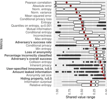
Figure 12 shows the distribution and average values for the shared value range score across all scenarios. We note that none of the per-graph metrics have a high shared value range. As a result, even for comparisons between graphs, per-node metrics are recommended. Only three metrics have a shared value range score above 0.5 as well as a mono-tonicity score above 0.5:pearson correlation,absolute error, and

normalized variance. 0.95 0.9 0.85 0.8 0.7 0.6 0 1 Pearson correlation 0.37 0.18 0.11 0.06 0.01 -0.01

(a)Pearson correlation, Caida, vary-ing aux ratio, YG, ID rem., range=1.0 0.95 0.9 0.85 0.8 0.7 0.6 0 1 Pearson correlation 0.13 0.11 0.1 0.08 0.04 0.02

(b)Pearson correlation, Manufactur-ing, varying aux ratio, JLSB, t-means, range=1.0 0.95 0.9 0.85 0.8 0.7 0.6 0 2000 4000 # of nodes 1.2k 1.4k 1.4k 1.4k 1.4k 1.4k

(c) Anonymity set size, Caida, varying aux ratio, YG, ID rem., range=0.59 0.95 0.9 0.85 0.8 0.7 0.6 50 100 # of nodes 88.4 88.7 89.1 89.4 90.4 91.2

(d) Anonymity set size, Manufac-turing, varying aux ratio, JLSB, t-means, range=0.01

Fig. 11. Shared value range:pearson correlationin the top row has a

consistent value range across scenarios, while theanonymity set sizein

the bottom row uses a different value range (y axis) for each scenario.

Relative entropy Information surprisal

Hiding property, t=0.5Anonymity set size

Amount leaked information

User-specified innocence, t=0.5Inherent privacy

Collision entropy Adversary's overall success

Percentage incorrectly classifiedLoss of anonymity

Min entropy Conditional privacy

Adversary's success rateMax entropy

Incorrectness Conditional entropyMutual information Quantiles on entropy, q=0.001Entropy Conditional privacy lossMean squared error Norm. varianceNorm. entropy Absolute error Pearson correlation 0.00 0.25 0.50 0.75 1.00

Shared value range

Metrics

Fig. 12. Box plot showing the ranking of privacy metrics according to their shared value range scores.

6.3 Analysis of Factors Influencing Evenness and Shared Value Range

We again used MARS and linear regression to analyze how much of the variation in evenness and shared value range can be explained by characteristics of the dataset, anonymization, and de-anonymization algorithms. Tables 5 and 6 show that, similar to monotonicity, evenness and shared value range are mostly influenced by the metrics and not by the other components of our experiments.

The linear regression confirmed that the anonymizer, de-anonymizer, dataset and graph type together account for under 20% of the variation in evenness (R2 _{= 0.194) and} under 17% of the variation in shared value range (R2 = 0.166). The graph statistics account for under 2% (R2 ₌

TABLE 5

MARS model showing which factors influence evenness

evenness = -0.018

+ 0.54 * metric Relative entropy

+ 0.4 * metric Quantiles on entropy, q=0.001 + 0.61 * metric Percentage incorrectly classified + 0.61 * metric Pearson correlation

+ 0.45 * metric Norm. variance + 0.22 * metric Norm. entropy + 0.45 * metric Mutual information + 0.41 * metric Min-entropy + 0.27 * metric Mean squared error + 0.33 * metric Max-entropy + 0.49 * metric Loss of anonymity + 0.31 * metric Inherent privacy + 0.48 * metric Information surprisal + 0.21 * metric Incorrectness + 0.41 * metric Entropy

+ 0.23 * metric Conditional privacy loss + 0.38 * metric Conditional privacy + 0.43 * metric Conditional entropy + 0.4 * metric Collision entropy + 0.06 * metric Anonymity set size + 0.53 * metric Adversary’s success rate + 0.54 * metric Adversary’s overall success + 0.16 * metric Absolute error

- 0.039 * anonymizer k-Symmetry + 0.15 * de-anonymizer DV + 0.2 * de-anonymizer JLSB + 0.2 * de-anonymizer KL + 0.33 * de-anonymizer NS + 0.23 * de-anonymizer YG + 3.1e-08 * max(0, 2e+06 - wedges) - 6.6e-09 * max(0, wedges - 2e+06) - 0.0011 * max(0, 94 - spectral norm)

0.015) of the variation in evenness and under 1% (R2 = 0.0006) of the variation in shared value range.

This replicates our finding for monotonicity and con-firms that evenness and shared value range are primarily influenced by the choice of metric, and not by the dataset or anonymization/de-anonymization algorithms.

7 R

: M

S

Based on our experimental results and the analysis in the previous sections, we can see that no single metric is the ideal metric for all scenarios. The metrics with the highest monotonicity are per-graph metrics, which do not provide information about the privacy levels of individual nodes in a graph. Most of the other metrics have very low monotonic-ity, and only seven metrics have an average monotonicity score of 0.5 or above. When considering evenness and shared value range in addition to monotonicity, only two metrics have high scores in all three criteria (pearson

cor-relationand normalized variance). Finally, another important

consideration is the semantics of metrics and their interpre-tation. In this regard, it is desirable to measure different aspects of privacy, for example in terms of the categories described in Section 3.4 [28].

Therefore, we recommend to combine several privacy metrics in a metrics suite. To allow for easy comparisons between anonymizing or de-anonymizing algorithms, and to be able to decide which provides the best or worst privacy levels, it is desirable to combine the metrics in a suite into

TABLE 6

MARS model showing which factors influence shared value range

shared value range = 0.22

+ 0.14 * metric Relative entropy

+ 0.31 * metric Quantiles on entropy, q=0.001 + 0.63 * metric Pearson correlation

+ 0.43 * metric Norm. variance + 0.44 * metric Norm. entropy + 0.31 * metric Mutual information + 0.36 * metric Mean squared error + 0.2 * metric Max-entropy - 0.077 * metric Inherent privacy + 0.13 * metric Information surprisal + 0.24 * metric Incorrectness - 0.15 * metric Hiding property, t=0.5 + 0.32 * metric Entropy

+ 0.34 * metric Conditional privacy loss + 0.14 * metric Conditional privacy + 0.28 * metric Conditional entropy - 0.055 * metric Collision entropy - 0.12 * metric Anonymity set size - 0.093 * metric Amount leaked information + 0.16 * metric Adversary’s success rate + 0.55 * metric Absolute error

- 0.063 * anonymizer HRG-DP - 0.07 * anonymizer WPINQ-DP - 0.15 * de-anonymizer DV - 0.15 * de-anonymizer JLSB - 0.18 * de-anonymizer KL + 0.12 * de-anonymizer NS + 0.049 * de-anonymizer YG

a single number. This is not a straightforward task because metrics have different scales of measurement and different directions (for some, higher values indicate higher privacy, for others, lower values). A simple average is therefore unlikely to yield good results, and any normalization has to carefully consider direction and value range.

7.1 Combining Metrics in a Metrics Suite

The problem of combining metrics is similar to a problem in operations research: given a set of alternatives and a number of criteria for each alternative, which alternative is best? Many methods have been proposed for multi-criteria decision analysis [33]. The simplest method is the weighted sum model (WSM), which ranks alternatives according to a weighted sum of the criteria values. However, this method is only applicable if the criteria are measured on the same scale and in the same units. The weighted product model (WPM) instead computes the relative importance Qi of each alternative i using a weighted product. Applied to the case of privacy metrics, each criterion j corresponds to one privacy metric, and the set of alternatives is the set of scenarios (e.g., anonymization algorithms or parameter settings) that need to be compared in terms of their privacy. According to [33], the relative importance of each alternative

iis computed as Qi= n Y j=1 (xij)wj,

where wj is the weight assigned to each metric, and

xij is a normalization of the metric value xij such that

xij = xij