This is an Open Access document downloaded from ORCA, Cardiff University's institutional
repository: http://orca.cf.ac.uk/125794/
This is the author’s version of a work that was submitted to / accepted for publication.
Citation for final published version:
Li, Kun, Liu, Jingying, Lai, Yukun and Yang, Jingyu 2019. Generating 3D faces using
multi-column graph convolutional networks. Computer Graphics Forum 38 (7) , pp. 215-224. file
Publishers page: http://dx.doi.org/10.1111/cgf.13830 <http://dx.doi.org/10.1111/cgf.13830>
Please note:
Changes made as a result of publishing processes such as copy-editing, formatting and page
numbers may not be reflected in this version. For the definitive version of this publication, please
refer to the published source. You are advised to consult the publisher’s version if you wish to cite
this paper.
This version is being made available in accordance with publisher policies. See
http://orca.cf.ac.uk/policies.html for usage policies. Copyright and moral rights for publications
made available in ORCA are retained by the copyright holders.
Pacific Graphics 2019
C. Theobalt, J. Lee, and G. Wetzstein (Guest Editors)
Volume 38(2019),Number 7
Generating 3D Faces using Multi-column Graph
Convolutional Networks
Kun Li1, Jingying Liu1, Yu-Kun Lai2and Jingyu Yang3†
1College of Intelligence and Computing, Tianjin University, Tianjin 300350, China 2Cardiff University, Wales, UK
3School of Electrical and Information Engineering, Tianjin University, Tianjin 300072, China
Figure 1:Reconstruction results of our multi-column graph convolutional networks (MGCNs).
Abstract
In this work, we introduce multi-column graph convolutional networks (MGCNs), a deep generative model for 3D mesh surfaces that effectively learns a non-linear facial representation. We perform spectral decomposition of meshes and apply convolutions directly in the frequency domain. Our network architecture involves multiple columns of graph convolutional networks (GCNs), namely large GCN (L-GCN), medium GCN (M-GCN) and small GCN (S-GCN), with different filter sizes to extract features at different scales. L-GCN is more useful to extract large-scale features, whereas S-GCN is effective for extracting subtle and fine-grained features, and M-GCN captures information in between. Therefore, to obtain a high-quality representation, we propose a selective fusion method that adaptively integrates these three kinds of information. Spatially non-local relationships are also exploited through a self-attention mechanism to further improve the representation ability in the latent vector space. Through extensive experiments, we demonstrate the superiority of our end-to-end framework in improving the accuracy of 3D face reconstruction. Moreover, with the help of variational inference, our model has excellent generating ability.
CCS Concepts
•Computing methodologies→Shape representations; Mesh models;
† Corresponding author: [email protected]. Postprint accepted by Pacific Graphics 2019
1. Introduction
Human faces contain rich information, such as individual identity, emotion and intention, and hence occupy a very important posi-tion in human visual percepposi-tion. 3D face reconstrucposi-tion is helpful to solve poses, expressions and missing features of faces from im-ages, and has a wide range of applications in computer vision and graphics, e.g., face recognition, face animation, and face tracking. However, obtaining a precise 3D face model is challenging because faces are highly variable, especially for non-linear changes due to complex expressions.
3D face models are often acquired by using a 3D scanner, but high-quality 3D scanners are expensive and complicated to operate. Statistical 3D face models, such as the 3DMM (3D Face Morphable Model) parametric model [BV99], provide prior knowledge of 3D faces through statistical analysis. This means a 3D face is repre-sented as a linear combination of 3D face basis vectors obtained by principal component analysis (PCA) on densely arranged 3D faces. However, the representation power of 3DMM-based meth-ods [BV99,BMVS04] is limited not only by the size of the training set, but also by its capability of capturing variations in different fa-cial expressions or poses, which often violate the linear assumption of PCA-based models. In addition, the PCA-based method is es-sentially a low-pass filter, which fails to restore the details of faces. With the development of deep learning, nonlinear 3D face mor-phable models show improved representation power. From this per-spective, the linear 3DMM representation is equivalent to a single-layer network, whereas the deep network architecture naturally in-creases the model capacity [TL18].
Previous works mostly tackle 3D face generation tasks in the Euclidean domain, but meshes are naturally in the non-Euclidean domain. Ranjanet al.[RBSB18] focused on non-Euclidean data
and introduced a versatile model that learns a non-linear represen-tation of 3D faces using spectral convolutions on a mesh surface, but this method cannot effectively capture multi-scale spatial infor-mation, resulting in the learned hidden layer vector having limited discrimination and generalization abilities.
In this paper, inspired by the work [CMS12] for image classi-fication, we propose a novel face representation and reconstruc-tion method with multi-column graph convolureconstruc-tional mesh autoen-coders, which can achieve higher quality reconstruction. Moreover, we propose a selective fusion module and utilize self-attention mechanism to better fuse features of different scales. This makes convolutions memory efficient and feasible to process high reso-lution meshes. Experimental results demonstrate that the proposed method provides significant improvement over the state-of-the-art generation methods on a standard dataset. An example of recon-struction results of our network is shown in Figure1. Our code will be released online.
The main contributions of this paper are summarized as follows:
• Multi-column graph convolutional networks (MGCNs). We
propose a MGCN architecture to effectively capture information at different scales on meshes, and learn a better latent space rep-resentation. The three columns correspond to filters with recep-tive fields of different sizes (large, medium, small), so that the
features learned by each column graph convolution are adaptive to large variations on face meshes such as eyes, nose and mouth.
• Selective fusion. We propose a learnable feature fusion method
on the basis of MGCNs. Combining self-attention mechanism makes fusion more intelligent. This method further boosts poten-tial representation of 3D faces in a low-dimensional latent space.
• Improved generation capabilities. Experimental results
demonstrate that our method achieves much better results in terms of reconstruction errors, compared with the state of the art. Remarkably, we can reduce reconstruction error from 0.845 to 0.390 on interpolation experiments. Simultaneously, our model can be used in a variational setting to sample a diverse range of face meshes from a known Gaussian distribution, as shown in Figure1.
2. Related Work 2.1. Face Representation
Face modeling is a challenging topic in computer vision snd graph-ics. Most methods use statistical priors to model the structure and expression of faces. However, facial variations are nonlinear in the real world,e.g., the variations in different facial expressions. Ex-isting work can be mainly divided into two categories: PCA-based linear approaches and deep learning based nonlinear approaches.
PCA-based Linear Approaches. The earliest face
parameter-ization model 3D Morphable Model (3DMM) was proposed by Blanz and Vetter [BV99], which is a statistical model of 3D facial shapes and textures. The 3D faces with only neutral expressions were captured in well-controlled conditions and obtained by laser scanning. The widely-used Basel Face Model (BFM) [PKA∗09] is
also built with 200 subjects in only neutral expressions. Lack of expression can be compensated for using the expression basis from FaceWarehouse [CWZ∗13]. There are various variants of 3DMM.
Yanget al.[GGSC96] used multiple PCA models, each of which
corresponds to a kind of expression. Amberget al.[AW92]
com-bined the neutral shape PCA model with the PCA model of ex-pression residuals obtained from neutral shapes. A similar model with an albedo model was proposed in the Face2Face framework [WJV∗04]. Tenaet al.[TDLTM14] presented a linear face
mod-eling approach that better generalizes to unseen data than tradi-tional holistic approaches and also allows click-and-drag interac-tion for animainterac-tion. Wuet al.[WBGB16] combined an anatomical
subspace with a local patch-based deformation subspace to realisti-cally model the facial performance of three actors. But their method uses personalized subspaces to capture shape details and therefore is not applicable to arbitrary target subjects.
Nonlinear 3D Face Models. Recently, some work proposed to
embed 3D face shapes by nonlinear parametric models with the power of deep learning methods. Conventional 3DMM is learned from a set of well-controlled 2D face images with associated 3D face scans, and represented by two sets of PCA basis functions. Due to the type and amount of training data, as well as the lin-ear bases, the representation power of 3DMM is limited. To ad-dress these problems, Tran and Liu [TL18] proposed an innovative framework to learn a nonlinear 3DMM model from a large set of unconstrained face images, without collecting 3D face scans. Feng
Kun Li et al. / Generating 3D Faces using Multi-column Graph Convolutional Networks 3
3.1. Overview
3D Face Representation. Given a collection of 3D face meshes,
we aim to obtain generated faces from the model. We represent a facial surface as a set of verticesVand edgesE.|V|=nvertices lie in 3D Euclidean space, so the coordinates of all the vertices form a matrixV∈Rn×3. The edges are represented using an adjacency matrixA∈ {0,1}n×nwhereai j=1 denotes an edge connection
between verticesviandvj, andai j=0 otherwise. An embedding M= (V,A)is realized by assigning 3D coordinates to the vertices
V, which is encoded as ann×3 matrixVcontaining the vertex
coordinates as rows.M= (V,A)is the input of network, and the network uses an encoder-decoder architecture to generate a new meshM′= (V′,A′)which can be expressed as a new sample.
Graph Convolution Networks. In order to deal with this
non-Euclidean data, we use graph convolution [DBV16] for feature learning. We first provide some background about this convolution. The Laplacian operator is discretized (using the distance-based equivalent of the cotangent formula [JSH12]) as an n×nmatrix
L=D−A, where the diagonal matrixDrepresents the degree of
each vertex inV asdii=∑jai j. The Laplacian is diagonalized by
the Fourier basisU∈Rn×n(sinceLis a real symmetric matrix) as
L=UΛUT, where the columns ofU= [u0,u1, . . . ,un−1]are the
orthogonal eigenvectors ofL, andΛ=diag([λ0,λ1, . . . ,λn−1])∈ Rn×n is a diagonal matrix with the associated real, non-negative
eigenvalues. The graph Fourier transform [Chu96] of the mesh ver-tices V∈Rn×3 is then defined as Vω=UTV, and the inverse
Fourier transform asV=UVω.
Graph convolution is defined in the graph Fourier trans-form domain, which contains eigenvectors Uof Laplacian
ma-trix L. The convolution in Fourier space is defined as x∗y=
UUTx⊗UTy, where ⊗ is the element-wise Hadamard product. It follows that a signalxis filtered bygθasy=gθ(L)x. An
efficient way to compute the spectral convolution is to parametrize
gθas a Chebyshev polynomial of orderK, given inputx∈Rn×Fin: yj= Fin
∑
i=1 K−1∑
k=0 θki,jTk(L˜)xi, (1)whereyjis the j-th feature ofy∈Rn×Fout, ˜L=2L/λmax−In is
a scaled Laplacian matrix.Inis then×nunit matrix.λmaxis the
maximum eigenvalue.Tkis the Chebyshev polynomial of orderK
and can be computed recursively asTk(x) =2xTk−1(x)−Tk−2(x), T0=1 andT1=x. Each convolution layer hasFin×Foutvectors of
Chebyshev coefficients,θi,j∈Rk, as trainable parameters.
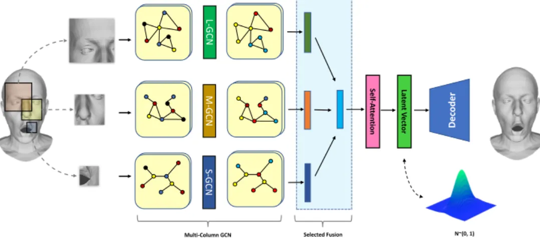
3.2. Multi-column Graph Convolution Networks
The overall structure of our MGCN is illustrated in Figure2. Our autoencoder consists of an encoder and a decoder. The detailed structures of the encoder and decoder are shown in Table 1 and Table 2, respectively. The encoder contains three parallel GCNs whose filters are with local receptive fields of different sizes. Each parallel GCN consists of 4 Chebyshev convolutional filters with
K Chebyshev polynomials. Each of the convolutions is followed
by a biased ReLU [GBB11]. The down-sampling layers, similar
etal.[FWS∗18]proposedastraightforwardmethodthat
simultane-ouslyreconstructsthe3Dfacialstructureandprovidesdense align-ment.Tanetal.[TGLX18]representedfacialexpressionswithdeep
learning,buttheirmethodusesfullyconnectedlayers,ratherthan convolutionsinthemeshdomain.
2.2. GraphConvolutionNetworks
Recent work about convolution on graphs can be categorized intospectralapproachesandnon-spectralapproaches.Spectral ap-proachesadoptaspectralrepresentationofgraphsthatreliesonthe eigen-decompositionoftheirLaplacianmatrices[KW17,DBV16]. ThecorrespondingeigenvectorsareregardedastheFourierbasisin theharmonicanalysisofspectralgraphtheory,andthenthespectral convolutionisdefinedastheelement-wiseproductoftwosignals’ Fouriertransformsonthe graph[BZSL14].However,asspectral approachesareassociatedwiththeircorrespondingLaplacian ma-trix,aspectralCNNmodellearnedononegraphcannotbedirectly transferredtoadifferentgraph,asitusuallyhasadifferent Lapla-cianmatrix,andspecialtreatmentisrequired[YSGG17].
Non-spectralapproachesaimtodefineconvolutionsdirectlyon a graph with local neighbors in a spatial or manifold domain. Thekeyfornon-spectralapproaches isto defineas eto fshared weightsapplied to the neighbors of each vertex [AT16]. Duve-naudetal.[DMAI∗15]computedaweightmatrixforeachvertex
andmultipliedit tothe neighbors,followedby asumoperation. Inductiverepresentationlearning ongraphs[HYL17] introduced aninductiveframeworkbyapplyingaspecificaggregatoroverthe neighbors,suchasthemax/meanoperatororarecurrentneural net-work(RNN).
However,thesegraphconvolutionnetworksarenotdirectly ap-plicableto3Dmeshes.CoMA[RBSB18] usedtruncated Cheby-shevpolynomials[DBV16]formeshconvolutions,butitisdifficult tocapturefeaturesofalldifferentscales. Toaddress these prob-lems,inthis work,weproposeanovelmulti-columngraph con-volutionalnetwork(MGCN)inspiredbymicrocolumnsofneurons inthecerebralcortex,inwhichwecombineseveralgraph convo-lutionalcolumnstoformaMGCN.Eachcolumninvolvesagraph convolutionalneuralnetworkwithmesh-baseddown-samplingand up-samplinglayerstoextractfeatureswithreceptivefieldsof dif-ferentsizes.Wealsoexploitself-attentionmechanismto capture non-localrelationships.Overall, weobtainacompletemesh au-toencoderstructuretorepresent highlycomplex3Dfaces,which outperformsexistingstateoftheart.
3. Methodology
Thissectiondescribesthe frameworkand thedetailsofour pro-posedmethod.Firstly,wedefinea3 Df acer epresentationwhich usesconvolutionallayerswithgraphconvolutionoperatorsto rep-resentfaces(Section3.1).Then,weelaboratethenetwork architec-tureandthelossfunctiondesignedspeciallyforminimizingerrors (Section3.2).Finally,wegivevariationalautoencoderformulation thathasgenerationcapabilities(Section3.3).
L -GC N M -GC N S -GC N
Multi-Column GCN Selected Fusion
Se lf-At te n tio n La ten t Ve ct o r De co d e r N~(0, 1)
Figure 2:Overview of our pipeline: 1) A multi-column GCN, includingL-GCN,M-GCN, andS-GCN, 2) Selective fusion for feature fusion from different column graph convolutions, 3) Self-attention mechanism to explore local features across spatial dimensions to improve the representation ability of deep models, 4) Variational loss with latent vector.
to [RBSB18], are interleaved between convolutional layers. Each
down-sampling rate is approximately 1/4. The encoder transforms the face mesh fromRn×3to a 64 dimensional latent vector using a
fully connected layer at the end. The decoder is a mirrored struc-ture of the encoder. We concatenate a selective fusion unit after the parallel structure, where the extracted features are selectively blended. Moreover, we explore local features across spatial dimen-sions to improve the representation ability of deep models through self-attention mechanism.
Multi-column Architecture. Due to the characteristics of 3D
graph structure data, sample data usually contains features of dif-ferent sizes, hence filters with receptive fields of the same size are unlikely to capture characteristics of a graph at different scales. It is more natural to use filters with different sizes of local receptive field to learn the characteristics of graph structure data. Therefore, how to measure the receptive field in graph convolution is the key problem to determine network performance. We rethink the pro-cess of graph convolution: differentK values represent the range
of nodes involved in the convolution process of graphs, and hence can control the convolution range of graphs. The larger the range of graphs is, the larger the scope in the original mesh space is, sim-ilar to the size of different receptive fields in 2D convolution by selecting different ranges.
In our MGCN, for each column, we use the filters of different sizes to extract features of different scales. For instance, filters with larger receptive fields (i.e., largerK) are more useful for extract-ing large-scale features, while filters with smaller receptive fields are more useful for extracting subtle and fine features. We divide the multi-column structure into three types: large graph convolu-tion network (L-GCN), medium graph convolution network ( M-GCN), and small graph convolution network (S-GCN), which are
sufficient in practice, although more or fewer columns may also be used. This approach can also be seen as multi-scale decomposition. We further propose a selective fusion method to integrate them.
Selective Fusion. After multi-scale convolution, we can obtain
three feature maps for the input, denoted asZGCNi(i=1,2,3 for
L-GCN, M-GCN and S-L-GCN, respectively) containing feature infor-mation of different scales. How to integrate them effectively is the key to improve the performance of the whole network. The simplest way is to directly concatenate them, but the contribution of feature information to the whole is not equal at each scale. Therefore, we propose a selective fusion method to automatically learn fusion pa-rameters. We multiply each feature map by a learnable parameter
wiand constrain their sum to one:
Z= 3
∑
i=1 wiZGCNi, s.t. 3∑
i=1 wi=1, (2) wherewiis the learnable parameter corresponding to the weightof thei-th column, andZGCNi is the feature map for the column.
wi can be seen as the importance of features at different scales.
These weights are optimized during training, which determine the importance of different scales to help generate better latent vectors.
Self-Attention. Discriminant feature representations are essential
for feature embedding, which could be obtained by capturing long-range contextual information. TheC-dimensional latent vectorZ
can be viewed as a feature map of sizeC×1. The attention mod-ule encodes a wider range of contextual information into local fea-tures, and thus enhances their representation capability. Following the self-attention operation in Figure3, we use a generic module in deep neural network as:
Oi= 1 N
∑
∀ih Ai,Bj t Zj +Zi, (3)whereNis a normalization term (defined later),Zis the local fea-ture map from the embedding module andO∈RC×1is the output
with the same size asZ. We generate two new feature mapsAand
BfromZby different 1×1 convolutions, where{A,B} ∈RC×1.
Aiand Bj are local features at different positions. Definehas a
function to compute a score which represents pairwise relationship. We use a Gaussion function with softmax for the pairwise function
h[WGGH18]:
h Ai,Bj=exp Ai·Bj. (4)
Kun Li et al. / Generating 3D Faces using Multi-column Graph Convolutional Networks 5
After that we can get the attention maph Ai,Bj∈RC×C. The
funcitont in Eq. (3) is a scale function implemented by a 1×1 operator, and hencet Zjcomputes a representation of inputZat
the position j. Then we perform a matrix multiplication between
the attention map andt Zj, and the result belongs toRC×1. It can
be inferred that the resulting feature at each position is a weighted sum of the features at all positions and original features. The nor-malization termNin equation5is defined as
N=
∑
∀j h Ai,Bj
. (5)
We also add residual connection [HZRS16] for the self-attention block to make it more efficient. This block learns to efficiently find global, long-range dependencies within internal representations of feature maps. Through self-attention, we can better explore latent vector generative capabilities on the basis of MGCNs.
Table 1:Encoder Architecture.
Layer Input size Output size Convolution 5023×3 5023×16 Down-Sampling 5023×16 1256×16 Convolution 1256×16 1256×16 Down-Sampling 1256×16 314×16 Convolution 314×16 314×16 Down-Sampling 314×16 79×16 Convolution 79×16 79×32 Down-Sampling 79×32 20×32 Fully Connected 20×32 64
Table 2:Decoder Architecture.
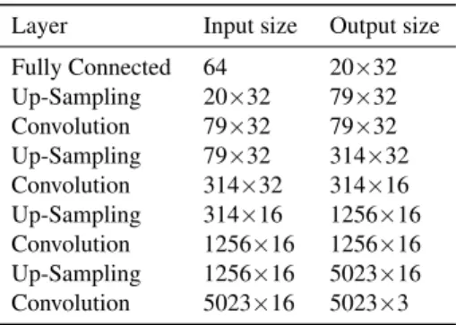
Layer Input size Output size Fully Connected 64 20×32 Up-Sampling 20×32 79×32 Convolution 79×32 79×32 Up-Sampling 79×32 314×32 Convolution 314×32 314×16 Up-Sampling 314×16 1256×16 Convolution 1256×16 1256×16 Up-Sampling 1256×16 5023×16 Convolution 5023×16 5023×3
Loss Function.In our multi-column graph convolutional network,
we use the per-vertex Euclidean distance between the predicted mesh and the ground-truth mesh to represent the reconstruction er-ror because we find that better convergence can be obtained with this loss in our problem. It is defined as
l=kM −D(Z)k2. (6) Ma tMu l So ft ma x Ma tMu l In p u t Ad d
Figure 3:Self-attention mechanism
3.3. Variational Mesh Autoencoder
Generative models have made great progress in recent years. The variational auto-encoder (VAE) is a recently introduced latent vari-able generative model, which combines variational inference with deep learning. However VAEs are mostly applied directly to 2D im-ages. Traditional methods [HKM15] use probabilistic inference for 3D model generation (synthesis), but they are only suitable for spe-cific 3D shapes. Our model not only has excellent reconstruction results but also has the ability to generate new shapes. Different from previous generative models, our model uses a MGCN with self-attention mechanism to better model high resolution details.
We draw on the ideas of VAE. VAE modifies the conventional auto-encoder framework in two key ways. First, a deterministic in-ternal representationZ(provided by the encoder) of an inputXis
replaced with a posterior distributionq(Z|X). Inputs are then re-constructed by samplingZfrom this posterior and passing them
through a decoder. To make sampling easy, the posterior distribu-tion is usually parametrized by a Gaussian with its mean and vari-ance predicted by the encoder. Second, to ensure that the model can sample from any point of the latent space and still generate valid and diverse outputs, the posteriorq(Z|X)is regularized with itsKLdivergence from a prior distributionp(Z).
Although 3D faces can be sampled from our convolutional mesh autoencoder, the distribution of the latent space is not known. Therefore, sampling requires a mesh to be encoded in that space. In order to constrain the distribution to normal distribution of the la-tent space, we add a variational loss to our model. So we minimize the loss:
l=kM −D(Z)k2+wkldKL(N(0,1)kq(Z|M)), (7) whereZis the latent representation of faceM, andwkld=0.001 is the weight of theKLdivergence loss. The first term minimizes the ℓ2reconstruction error, and the second term enforces a unit Gaus-sian priorN(0,1)with zero mean on the distribution of latent vec-torsq(Z). This enforces the latent space to be a multivariate Gaus-sian.
4. Experimental Results
In this section, we first evaluate the performance of our MGCNs in Section 4.1 which is compared with state-of-the-art methods, and whereMistheoriginalmesh,D(·)isthedecoder,andZisthe
la-tentrepresentationoffacemeshM.Thegoalofourlossfunction istomakethereconstructedshapeascloseaspossibletothe in-put.Thelossfunctionisoptimizedviabatch-basedstochastic gra-dientdescentand back-propagation,typically fortrainingneural networks.
Table 3:Interpolation comparison. Errors are in millimeters.
Ours CoMA [RBSB18] PCA
Mean Error 0.390±0.358 0.845±0.994 1.639±1.638
Median Error 0.383 0.496 1.101
Table 4:Extrapolation comparison. Errors are in millimeters.
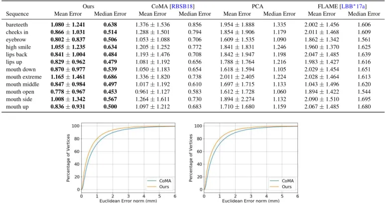
Ours CoMA [RBSB18] PCA FLAME [LBB∗17a]
Sequence Mean Error Median Error Mean Error Median Error Mean Error Median Error Mean Error Median Error
bareteeth 1.080±1.241 0.638 1.376±1.536 0.856 1.954±1.888 1.335 2.002±1.456 1.606 cheeks in 0.866±1.031 0.514 1.288±1.501 0.794 1.854±1.906 1.179 2.011±1.468 1.609 eyebrow 0.802±0.837 0.506 1.053±1.088 0.706 1.609±1.535 1.090 1.862±1.342 1.561 high smile 1.055±1.235 0.634 1.205±1.252 0.772 1.841±1.831 1.246 1.960±1.370 1.625 lips back 0.841±1.004 0.484 1.193±1.476 0.708 1.842±1.947 1.198 2.047±1.485 1.639 lips up 0.829±0.962 0.479 1.081±1.192 0.656 1.788±1.764 1.216 1.983±1.427 1.616 mouth down 0.870±0.977 0.539 1.050±1.183 0.654 1.618±1.594 1.105 2.029±1.454 1.651 mouth extreme 1.165±1.461 0.686 1.336±1.820 0.738 2.011±2.405 1.224 2.028±1.464 1.613 mouth middle 0.847±0.984 0.497 1.017±1.192 0.610 1.697±1.715 1.133 1.043±1.496 1.620 mouth open 0.778±0.967 0.453 0.961±1.127 0.583 1.612±1.728 1.060 1.894±1.422 1.544 mouth side 1.008±1.342 0.567 1.264±1.611 0.730 1.894±2.274 1.132 2.090±1.510 1.695 mouth up 0.836±0.931 0.500 1.097±1.212 0.683 1.710±1.680 1.159 2.067±1.485 1.680 (a) (b)
Figure 4: Cumulative Euclidean error histograms using CoMA and our MGCNs for Interpolation (a) and Extrapolation (b) experiments.
then perform an ablation study to analyze the effect of different components of our approach and the sensitivity of parameters in Section 4.2. Finally, we show a diverse range of face meshes sam-pled from the latent space to verify the generation ability of our network in Section 4.3.
Dataset. We use the CoMA dataset [RBSB18] to perform
var-ious ablation and comparison experiments. This dataset contains 20,466 3D meshes, each of which has about 120,000 vertices, and captures 3D sequences of 12 subjects of different age groups, each of whom performs 12 different expressions. These expressions are chosen such that they are extreme, causing a lot of facial tissue de-formation. These expressions are not only complex, but also asym-metric, so the task of reconstruction is a challenge. Moreover, none of these expressions are correlated with each other. The expres-sion sequences in our dataset arebareteeth, cheeks in,eyebrow, high smile,lips back,lips up,mouth down,mouth extreme,mouth middle, mouth open,mouth side andmouth up. The data is
pre-processed using a sequential mesh registration method [LBB∗17b]
to reduce the dimensionality to 5023 vertices.
Implementation Details. We utilize the deep learning
frame-work Keras with Tensorflow [ABC∗16] backend to implement
MGCNs and use NVIDIA GeForce GTX 1080 Ti GPU to complete all experiments. We train our method for 400 epochs with a learn-ing rate of 1e-4 and a learnlearn-ing rate decay of 0.99 every epoch. We use stochastic gradient descent (SGD) with a momentum of 0.9, which optimizes the loss function between the output mesh and the ground-truth mesh. We useℓ2regularization on the weights of
the network with weight decay of 5e-4. For network architecture, we set latent dimension as 64, and S-GCN, M-GCN and L-GCN use Chebyshev filtering with K=2,6,10, respectively. We have four graph convolution layers for each column, and the number of channels corresponding to them are 16, 32, 64, 64, respectively. Each convolution is followed by a batch normalization [IS15] and ReLU [NH10] activation function.
Evaluation Metrics. To evaluate the performance of the
pro-posed method, we adopt two mainstream evaluation metrics: Eu-clidean distance mean error with standard deviation, and median error. The mean error in term of Euclidean distanceebetween
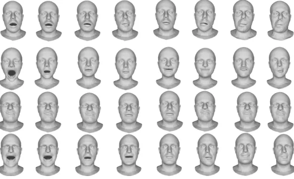
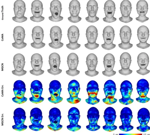
Kun Li et al. / Generating 3D Faces using Multi-column Graph Convolutional Networks 7 Gr ou nd Tr ut h Co M A M GCN Co M A Er r. M GCN E rr.
Figure 5:Qualitative results for the interpolation experiment.
constructed meshM′and original meshMis defined as: e M,M′ =1 n n
∑
i=1 vi−v′i 2. (8)Extrapolation Experiment. In order to measure the
generaliza-tion ability of the model, in addigeneraliza-tion to CoMA, we further compare the proposed method with two competitive models: PCA [BV99] and FLAME [LBB∗17a] in Table4. For comparison, we train the
expression model of FLAME on the CoMA dataset [RBSB18]. The FLAME reconstructions are obtained with latent vector size of 64. The latent vectors encoded using the PCA model and our mesh autoencoder are also of size 64, for fair comparison. We compare the performance using the mean, standard deviation, and median of Euclidean distance errors. We perform 12 fold cross validation, one for each expression. For each experiment, we split the CoMA dataset [RBSB18] according to a certain expression. The dataset is then divided into unseen data (faces of the selected expression) and seen data (faces of remaining expressions). As shown in Ta-ble4, our model performs better than the state-of-the-art methods on all expression sequences. Figure6shows visual inspection of the qualitative results. The cumulative Euclidean error histogram is shown in Figure4b. For a 1 mm accuracy bound, our MGCN captures 75.8% of the vertices, which is better than 61.2% of the CoMA method.
4.2. Ablation Study
We study the effect of each component which may affect exper-imental results in our approach on the CoMA dataset [RBSB18]. All the results are obtained over the input size of 5023×3. ThemedianerrorisdefinedasthemedianvalueofEuclideanerrors
ofallvertices.
4.1. Comparison
Interpolation Experiment. In order to evaluate the face
re-constructioncapabilityoftheproposedmethod,wecompareour method with CoMA [RBSB18] that introduces a convolutional meshautoencoderconsistingofmeshdownsamplingandmesh up-samplinglayerswithfastlocalizedconvolutionalfiltersdefinedon themeshsurface,aswellasbaselinePCAmethod.Weevaluatethe comparedmethodsusingthecorrespondingreleasedcodeand pa-rameterstoensuretheirperformance.Moreover,wedividethefull datasetintoatrainingsetandatestsetwitharatioof9:1.Themean errorandstandarddeviationforper-vertexEuclideandistanceon thetestsetaregivenin Table3.Weobservethatthe errorvalue ofourreconstructionresultis53.8%lowerthanCoMA.Figure4a isthecumulativeEuclideanerrorhistogram,showingthe propor-tionofvertices(y-axis)withingivenerrorbounds(x-axis).Fora
1mmaccuracybound,ourMGCNcaptures81.1%ofthevertices whiletheCoMAmodel[RBSB18]onlycaptures72.3%.Visual in-spectionofthequalitativeresultsinFigure5showsthatour recon-structedmeshesaremorerealisticandreasonable.
Table 5:The performances of different variants of our method.w/ means with.
Method Mean Error Std
Single-Column 0.875 0.613
Single-Column w/ attention 0.673 0.669
Multi-Column 0.571 0.632
Multi-Column w/ attention 0.523 0.523 Multi-Column w/ fusion 0.372 0.477 Multi-Column w/ attention + fusion 0.297 0.348
Component Module Analysis. In this section, we perform an
ablation study to analyze the effect of different components of our approach. In our method, we have three novel designs in-cluding multi-column graph convolution, selective fusion and self-attention, which greatly improve the representation ability of our method. To investigate the effectiveness of these three designs, Ta-ble5presents the performances of different variants of our learning method. From Table5, it can be observed that multi-column graph convolution structure is consistently better than single-column graph convolution structure. Self-attention plays a role in both structures to improve the network’s performance, which attributes to its ability to extract non-local relations in the latent vector. This kind of non-local relation is essential in generating tasks to ob-tain more detailed results. It should be emphasized that the selec-tive fusion component improves the network greatly in the multi-column structure, reducing error by nearly 0.2, which proves that our proposed fusion method is very effective. Overall, the combina-tion of multi-column graph convolucombina-tion structure, selective fusion and self-attention achieves satisfactory results in 3D face generat-ing tasks.
To explore how different scales of convolution affect network performance, we decode each column separately. As shown in Ta-ble6, we decode feature maps of different convolution kernel sizes, including 2, 4, 6, 8, 10, 12, respectively. It can be seen that convo-lution kernels which are either too large or too small do not work well. Although moderate sized convolution kernels show good per-formance, there is still a big gap with the result of multi-column convolution (shown in Table5).
We further compare multi-column GCNs with different numbers of layers in Table7to study how the network complexity affects the performance. We can see that, the 4-layer architecture we used achieves the best performance. The network may not have enough learning capability if the number of layers is too small, and over-fitting becomes an issue when the number of layers is too large, leading to worse performance on the test set.
Sensitivity Analysis. In particular, for multi-column structure,
we further verify whether differentKchoices have an impact on
the robustness of the network through sensitivity analysis of pa-rameters. Then, we select the bestKfor all our experiments. From
Table8, we can find that various filter parameters for the multi-column structure are consistently better than the single-multi-column ver-sion (shown in Table5). And the optimal parameters are 2,6,10. It is observed that if the difference betweenKvalues of each column
is too large or too small, it will not produce the best performance.
We believe that the appropriateKvalues should be in line with the
relative stability and increment (from S-GCN to L-GCN), so that the network can capture information of different scales to achieve the best performance. For the case of same values forK1,K2, and K3, the improvement of the network is not significant, because each
column captures information of the same scale.
Table 6:The performances of single column with different filter size K.
K 2 4 6 8 10 12
Mean Error 1.070 0.988 0.900 0.947 0.875 0.993
Std 0.528 0.669 0.441 0.794 0.613 0.284
Table 7:The performances of proposed multi-column GCN with
different network depths.
Depth 2 3 4 5 6
Mean Error 0.544 0.319 0.297 0.439 0.542 Std 0.297 0.512 0.348 0.231 0.406
Table 8:Sensitivity analysis for different filter size K.
(K1,K2,K3) Mean Error Std (1, 2, 3) 0.309 0.371 (2, 4, 6) 0.302 0.366 (2, 8, 14) 0.300 0.361 (6, 6, 6) 0.632 0.685 (2, 6, 10) 0.297 0.348 4.3. Sampling the Latent Space
To verify the generating ability of MGCNs when combined with variational loss, we can control the size of the elements in the hid-den vector, so that the decoder has the ability of generation and generates more discriminant samples. Figure7demonstrates the di-versity of face meshes sampled from the latent space. LetEbe the
encoder andDbe the decoder. We first encode a face mesh from our test set in the latent space to obtain a feature vectorZ=E(F). Then, we vary each component of the latent vector as ˜Zi=Zi+ε.
Finally, we use the decoder to transform the latent vector into a reconstructed mesh ˜F=D(Z˜). Here, we extend or contract the latent vector along different dimensions by a factor of 0.3, i.e.,
˜
Zi= (1+0.3j)Zi, wherej∈[−4,4]is the step, and the mean face F0is shown in the middle of each row.
5. Conclusions
In this paper, we propose multi-column graph convolution networks (MGCNs) for 3D face representation, reconstruction and genera-tion. A MGCN contains three different kinds of convolutions,i.e., large graph convolution network (L-GCN), middle graph convolu-tion network (M-GCN), and small graph convoluconvolu-tion network (S-GCN) to capture different scales of features. Moreover, we propose a selective fusion module and utilize self-attention mechanism to
Kun Li et al. / Generating 3D Faces using Multi-column Graph Convolutional Networks 9
better integrate features of different scales. The interpolation and extrapolation experiments demonstrate that the proposed method is more robust and provides significant improvement over the state-of-the-art methods on a standard dataset. Our current approach re-stricts fusion at the feature vector level. We will investigate more detailed selective fusion where each feature dimension has its own weights in the future. Since our method does not explicitly use face-specific domain knowledge, our method is not restricted to 3D faces. In the future, we will extend the proposed method to the 3D human body generation task.
Acknowledgements
This work was supported in part by the National Natural Science Foundation of China (Grant 61571322 and 61771339), and Tianjin Research Program of Application Foundation and Advanced Tech-nology under Grant 18JCYBJC19200.
References
[ABC∗16] ABADIM., BARHAM P., CHEN J., CHEN Z., DAVISA.,
DEANJ., DEVINM., GHEMAWATS., IRVINGG., ISARDM., KUD -LUR M., LEVENBERGJ., MONGAR., MOORES., MURRAYD. G.,
STEINERB., TUCKERP. A., VASUDEVAN V., WARDENP., WICKE
M., YUY., ZHANGX.: Tensorflow: A system for large-scale machine learning. InUSENIX Symposium on Operating Systems Design and Im-plementation (OSDI)(2016).6
[AT16] ATWOOD J., TOWSLEY D. F.: Diffusion-convolutional neu-ral networks. InAdvances in Neural Information Processing Systems (2016).3
[AW92] ADELSONE. H., WANGJ. Y. A.: Single lens stereo with a plenoptic camera. IEEE Transactions on Pattern Analysis and Machine Intelligence 14(1992), 99–106.2
[BMVS04] BLANZV., MEHLA., VETTERT., SEIDELH.-P.: A sta-tistical method for robust 3D surface reconstruction from sparse data. Proceedings. 2nd International Symposium on 3D Data Processing, Vi-sualization and Transmission (3DPVT)(2004), 293–300.2
[BV99] BLANZV., VETTERT.: A morphable model for the synthesis of 3D faces. InSIGGRAPH(1999).2,7
[BZSL14] BRUNA J., ZAREMBAW., SZLAMA., LECUNY.: Spec-tral networks and locally connected networks on graphs. CoRR abs/1312.6203(2014).3
[Chu96] CHUNGF. R. K.:Spectral Graph Theory. 1996.3
[CMS12] CIRESAND. C., MEIERU., SCHMIDHUBERJ.: Multi-column deep neural networks for image classification. InIEEE Conference on Computer Vision and Pattern Recognition(2012), pp. 3642–3649.2 [CWZ∗13] CAOC., WENGY., ZHOUS., TONGY., ZHOUK.:
Face-warehouse: A 3D facial expression database for visual computing.IEEE Transactions on Visualization and Computer Graphics 20, 3 (2013), 413–425.2
[DBV16] DEFFERRARDM., BRESSONX., VANDERGHEYNSTP.: Con-volutional neural networks on graphs with fast localized spectral filter-ing. InAdvances in Neural Information Processing Systems(2016).3 [DMAI∗15] DUVENAUD D. K., MACLAURIN D., AGUILERA
-IPARRAGUIRREJ., GÓMEZ-BOMBARELLIR., HIRZEL T., ASPURU
-GUZIK A., ADAMS R. P.: Convolutional networks on graphs for learning molecular fingerprints. In Advances in Neural Information Processing Systems(2015).3
[FWS∗18] FENGY., WUF., SHAOX., WANGY., ZHOUX.: Joint 3D
face reconstruction and dense alignment with position map regression network. InEuropean Conference on Computer Vision (ECCV)(2018).
3
[GBB11] GLOROTX., BORDESA., BENGIOY.: Deep sparse rectifier neural networks. InProceedings of the fourteenth international confer-ence on artificial intelligconfer-ence and statistics(2011), pp. 315–323.3 [GGSC96] GORTLERS. J., GRZESZCZUKR., SZELISKI R., COHEN
M. F.: The lumigraph. InSIGGRAPH(1996).2
[HKM15] HUANGH., KALOGERAKIS E., MARLINB. M.: Analysis and synthesis of 3D shape families via deep-learned generative models of surfaces.Comput. Graph. Forum 34(2015), 25–38.5
[HYL17] HAMILTONW. L., YINGZ., LESKOVECJ.: Inductive repre-sentation learning on large graphs. InAdvances in Neural Information Processing Systems(2017).3
[HZRS16] HEK., ZHANGX., RENS., SUNJ.: Deep residual learning for image recognition.IEEE Conference on Computer Vision and Pattern Recognition (CVPR)(2016), 770–778.5
[IS15] IOFFES., SZEGEDYC.: Batch normalization: Accelerating deep network training by reducing internal covariate shift. InInternational Conference on Machine Learning (ICML)(2015).6
[JSH12] JACOBSONA., SORKINE-HORNUNGO.: A Cotangent Lapla-cian for Images as Surfaces. Tech. rep., 2012.3
[KW17] KIPFT. N., WELLINGM.: Semi-supervised classification with graph convolutional networks.CoRR abs/1609.02907(2017).3 [LBB∗17a] LI T., BOLKART T., BLACK M. J., LI H., ROMEROJ.:
Learning a model of facial shape and expression from 4d scans. ACM Transactions on Graphics 36, 6 (2017), 194:1–194:17.6,7
[LBB∗17b] LI T., BOLKART T., BLACK M. J., LI H., ROMEROJ.:
Learning a model of facial shape and expression from 4d scans. ACM Transactions on Graphics 36(2017), 194:1–194:17.6
[NH10] NAIRV., HINTON G. E.: Rectified linear units improve re-stricted boltzmann machines. InInternational Conference on Machine Learning (ICML)(2010).6
[PKA∗09] PAYSANP., KNOTHER., AMBERGB., ROMDHANIS., VET
-TERT.: A 3D face model for pose and illumination invariant face recog-nition. InIEEE Intl. Conf. on Advanced Video and Signal Based Surveil-lance(2009), pp. 296–301.2
[RBSB18] RANJANA., BOLKARTT., SANYALS., BLACKM. J.: Gen-erating 3D faces using convolutional mesh autoencoders. InEuropean Conference on Computer Vision (ECCV)(2018).2,3,4,6,7
[TDLTM14] TENAJ. R., DELATORREF., MATTHEWSI.: Interactive region-based linear 3D face models, 2014. US Patent 8,922,553.2 [TGLX18] TANQ., GAOL., LAIY.-K., XIAS.: Variational
autoen-coders for deforming 3D mesh models. InIEEE Conference on Com-puter Vision and Pattern Recognition (CVPR)(2018), pp. 5841–5850. 3
[TL18] TRAN L., LIU X.: Nonlinear 3D face morphable model. IEEE Conference on Computer Vision and Pattern Recognition (CVPR) (2018), 7346–7355.2
[WBGB16] WU C., BRADLEY D., GROSS M., BEELER T.: An anatomically-constrained local deformation model for monocular face capture.ACM Transactions on Graphics (TOG) 35, 4 (2016), 115.2 [WGGH18] WANGX., GIRSHICKR. B., GUPTAA., HEK.: Non-local
neural networks.IEEE/CVF Conference on Computer Vision and Pattern Recognition (CVPR)(2018), 7794–7803.4
[WJV∗04] WILBURNB., JOSHIN., VAISHV., LEVOYM., HOROWITZ
M. A.: High speed video using a dense camera array. InIEEE Confer-ence on Computer Vision and Pattern Recognition (CVPR)(2004).2 [YSGG17] YIL., SUH., GUOX., GUIBASL. J.: SyncSpecCNN:
Syn-chronized spectral cnn for 3D shape segmentation.IEEE Conference on Computer Vision and Pattern Recognition (CVPR)(2017), 6584–6592.3
Gr ou nd Tr ut h Co M A M GCN Co M A Er r. M GCN E rr.
Figure 6:Qualitative results for the extrapolation experiment.
Co m po nen t 3 Co m po nen t 2 Co m po nen t 1 j=0(mean) j=-1 j=-2 j=-3 j=-4 j=1 j=2 j=3 j=4
Figure 7:Sampling from the latent space of the mesh autoencoder around the mean face j = 0 along 3 different components.