The Monetary and Fiscal History of
Brazil, 1960–2016
∗
Joao Ayres
†Marcio Garcia
‡Diogo Guillen
§Patrick Kehoe
¶December 20, 2018
Abstract
Brazil has had a long period of high inflation. It peaked around 100 percent per year in 1964, decreased until the first oil shock (1973), but accelerated again afterward, reaching levels above 100 percent on average between 1980 and 1994. This last period coincided with severe balance of payments problems and economic stagnation that followed the external debt crisis in the early 1980s. We show that the high-inflation period (1960–1994) was characterized by a combination of fiscal deficits, passive monetary policy, and constraints on debt financing. The transition to the low-inflation period (1995–2016) was characterized by improvements in all of these features, but it did not lead to significant improvements in economic growth. In addition, we document a strong positive correlation between inflation rates and seigniorage revenues, although inflation rates are relatively high for modest lev-els of seigniorage revenues. Finally, we discuss the role of the weak institutional framework surrounding the fiscal and monetary authorities and the role of mone-tary passiveness and inflation indexation in accounting for the unique features of inflation dynamics in Brazil.
∗This is a chapter in forthcoming book The Monetary and Fiscal History of Latin America. We
would like to thank Marcelo Abreu, P´ersio Arida, Edmar Bacha, Marco Bassetto, Tiago Berriel, Afonso Bevilaqua, Amaury Bier, Claudio Considera, Gustavo Franco, Fabio Giambiagi, Claudio Jaloretto, Joaquim Levy, Eduardo Loyo, Timothy Kehoe, Ana Maria Jul, Randy Kroszner, Pedro Malan, Rodolfo Manuelli, Andy Neumeyer, Juan Pablo Nicolini, Affonso Pastore, Murilo Portugal, Thomas Sargent, Teresa Ter-Minassian, Jos´e Scheinkman, Rog´erio Werneck, and participants at the “Monetary and Fis-cal History of Latin America” workshops held in the University of Chicago, LACEA-LAMES in Buenos Aires, PUC-Rio, Central Bank of Chile, and Inter-American Development Bank. This project was coor-dinated by Marcio Garcia.
†Inter-American Development Bank (IADB).
‡Pontifical Catholic University of Rio de Janeiro (PUC-Rio), CNPq, and FAPERJ. §Itau-Unibanco Asset Management.
1
Introduction
This chapter presents the monetary and fiscal history of Brazil between 1960 and 2016, with emphasis on the hyperinflation episodes. It describes the evolution of the Brazilian monetary and fiscal policy institutions and how they relate to episodes of macroeconomic instability and growth experience, focusing on the high-inflation period (pre-1994) and two stabilization plans: the Government Economic Action Plan (PAEG, an abbreviation for Plano de A¸c˜ao Econˆomica do Governo) and the Real Plan. The PAEG, in 1964, stabilized inflation around 100 percent per year, whereas the Real Plan, in 1994, stabilized inflation around 90 percent per month after six failed attempts in over a decade. The analysis follows the conceptual framework in chapter 2 by focusing on the government budget constraint.
A summary of the period is illustrated in figure 1, which shows the evolution of real GDP per capita, inflation, and government deficits for the 1960–2016 period.1 Three
subperiods are identified: (1) 1960–1980: fast economic growth with high inflation and moderate deficits; (2) 1981–1994: slow growth with hyperinflation and high deficits; and (3) 1995–2016: moderate growth with low inflation and low deficits.2 The 1981–1994 subperiod stands out not only by its poor growth performance and hyperinflation but also by severe balance of payments problems, a common feature among highly indebted Latin American countries affected by the increase in international interest rates and the slowdown in international economic growth.
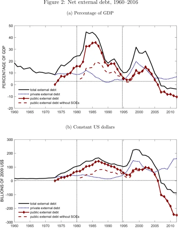
When relating the episodes of macroeconomic instability to the government fiscal and monetary policies, we observe the following: (1) both stabilization plans, PAEG in 1964 and the Real Plan in 1994, included measures to improve fiscal balances and were followed by increased access to debt financing; (2) the government policy to increase public investment in the wake of the first oil shock in 1973 explains the rapid increase in external debt that preceded the external debt crisis of 1983 seen in figure 2; and (3) the high-inflation periods (pre-1994) were characterized by the combination of fiscal deficits, passive monetary policy, and constraints on debt financing, while the transition to the low-inflation period (1995–2016) was associated with improvements in government fiscal balances, higher de facto independence of the monetary authority (as of this writing, Brazil still lacks a formally independent central bank), as well as much greater access to debt financing.
In comparison to other Latin American countries, the following two characteristics make the Brazilian experience rather unique: (1) a long period of high inflation, with annual inflation rates above 100 percent between 1980 and 1994; and (2) modest levels
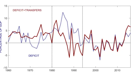
1AppendixCdiscusses the data and methodology. Our definition of “deficit” is the primary deficit
plus real interest payments on debt discounting for real GDP growth (see chapter 2), and throughout the chapter, we use the General Price Index from Getulio Vargas Foundation, IGP-DI, as our benchmark.
of deficits for very high underlying inflation rates. We discuss two features that may explain these unique characteristics of the Brazilian hyperinflation. The first is a poor institutional framework in which other public entities besides the monetary authority had indirect control over money issuance. We discuss that framework in section4.1. The second is the combination of a high degree of indexation in the economy to past inflation with a passive monetary policy.3 Together, these features created what was called at the
time inflation inertia, which could explain why the Brazilian hyperinflation was a much more protracted process than elsewhere and gave many the illusion that it could be cured without major improvements in the fiscal stance. We discuss that factor in section 4.2.
This chapter is organized as follows: in section 2, we present a summary of the government budget constraint, and in section 3, we provide a historical description of each of the subperiods 1960–1980, 1981–1994, and 1995–2016. In section4we discuss the evolution of the institutional framework involving both fiscal and monetary authorities and the genesis of inflation inertia, and in section 5, we present our final remarks and conclusion.
2
The government budget constraint
We are interested in analyzing the evolution of the government budget constraint for Brazil in 1960–2016. We attempt to match the variation in stocks (debt figures) with flows (fiscal deficits), duly accounting for valuation effects.4 Table 1presents a summary of the
results. In order to finance interest payments and primary deficits, the government can either issue domestic and external debt or issue money and receive seigniorage revenues. Transfers account for the residual.5
We divide the 1960–1980 subperiod into three parts: 1960–1964, 1965–1972, and 1973– 1980. In 1960–1964, markets for government debt securities were still underdeveloped, and the government faced restrictions on both domestic and external debt financing. Interest payments were low but primary deficits were on the rise, and had to be financed with seigniorage revenues. In 1964–1967, the stabilization plan PAEG implemented both fiscal and financial reforms, which reduced primary deficits and allowed the government to issue domestic debt securities. Those reforms account for the increase in domestic debt financing and the reduction in seigniorage revenues that we observe in the 1965– 1972 period. In 1973–1980, on the other hand, we observe a rise in both debt financing in external markets and seigniorage revenues, which were associated with higher interest
3Most prices, wages, taxes, and the exchange rate were indexed to past inflation. 4Mainly the effect of devaluations on foreign-currency-denominated or indexed debt.
5The sums of primary deficits and transfers is close to the measure of the primary deficit reported by
the Central Bank of Brazil starting in 1985, which is based on the public-sector borrowing requirements and is usually referred to as the primary deficitbelow the line. See appendixC.
payments on external debt and a significant rise in transfers, the residual.6 Fortunately,
in this case, we can explain what most of these transfers are. In the wake of the first oil crisis of 1973, the government implemented policies that aimed at boosting investment through external borrowing, and that was done mainly through state-owned enterprises (SOEs). The debt series that was used to compute the government budget constraint includes SOEs, but the primary deficit series does not. The increase in investment by SOEs, documented in table 2, accounts for a large fraction of the increase in transfers.7 Therefore, we argue that deficits at the time are better represented by adding the transfers to the reported primary deficits, which is reported in row 9 of table 1, labeled “primary deficits + transfers.”8
In 1981–1994, debt financing in external markets decreased sharply, and interest pay-ments on external debt increased as a reflection of the debt crisis that followed the increase in international interest rates. In that period, seigniorage revenues were used to finance the payments of both principal and interest of the external debt as well as the primary deficits.
The 1995–2002 period followed the agreement on the external debt renegotiations and the end of the hyperinflation in 1994. It showed a significant reduction in seigniorage revenues and a large improvement in primary and fiscal balances. Interest payments on external debt decreased, whereas interest payments on domestic debt increased. The 2003–2011 period continued to show primary and fiscal surpluses and low seigniorage revenues, and the external debt was replaced by domestic debt. As we will discuss, the pattern that we observe in 1994–2011 reflects changes in both monetary and fiscal policy institutions, with higher de facto independence of the central bank and greater control over the government budget. However, in the most recent period, 2012–2016, we observe a deterioration in fiscal balances that have been financed by a rapid increase in domestic debt.
In the sections that follow, we provide a detailed historical background that describes the fiscal and monetary policies adopted in the 1960–2016 period and that account for the evolution of the government budget constraint.
6Interest payments might be negative because we are discounting for growth rates in real GDP and
for the monetary correction of the debt.
7According to Werneck (1991), the average capital expenditures of SOEs for the 1973–1980 period
made up 7.4 percent of GDP, so our figures might be underestimating their importance. Nevertheless, both sources of data indicate a rapid increase in investments by SOEs in that period.
8By doing so, we approximate what the Central Bank of Brazil has done in its fiscal statistics starting
3
Historical description
3.1
1960–1980: fast growth with macroeconomic instability
Brazil went through important transformations during the first subperiod of our anal-ysis. It moved from being a rural society, in which 55 percent of the population lived in rural areas, to an urban society, with 68 percent of the population living in cities. Its production structure shifted toward the manufacturing sector, which increased its frac-tion of GDP from 32 to 41 percent, while the agricultural sector saw its fracfrac-tion of GDP reduced from 18 to 10 percent.9 It was a period of fast economic growth, with real GDP per capita increasing 4.6 percent per year on average (figure1a). However, it was also a period of macroeconomic instability, with a deep recession in the early 1960s, increasing external indebtedness following the first oil crisis in 1973, and nominal instability. In-flation rates rose in the beginning and reached levels around 100 percent in 1964, when the stabilization plan PAEG was implemented after a military coup.10 Inflation rates fell
significantly but started to accelerate again around the first oil crisis in 1973, returning to three-digit levels in 1980.11
To understand the fiscal and monetary policy institutions that were in place during these years, one should note that it was a period of heated debate regarding the role of the state in promoting economic development, during which the government undertook major national development plans, such as the Targets Plan in 1956–1961, the National Development Plan I in 1972–1974, and the National Development Plan II in 1975–1979. That process also led to a surge in the number of public banks, with nine out of twenty-three states creating their own banks between 1960 and 1964 to finance their fiscal deficits, and to the creation of some of the largest Brazilian SOEs, such as Eletrobras in 1962 and Telebras in 1972.12 As we discuss below, they would all play an important role in explaining the dynamics of the government budget constraint.
3.1.1 1960–1964
Before 1964, the government Treasury had direct control over money issuance through the Bank of Brazil (BB), which was both the bank of the government and a commercial bank.13 The main monetary policy instruments in use were the control over the monetary
base, subsidized credit to the industrial and agricultural sectors, and interventions in the foreign exchange market. Some of those interventions aimed to protect the local industry
9Data from the Brazilian Institute of Geography and Statistics (IBGE). 10The military dictatorship would last until 1985.
11For thorough analyses of that period, we refer to Orenstein and Sochaczewski (2014), Mesquita
(2014), Lago (2014), and Carneiro (2014).
12The other well-known Brazilian SOEs, Companhia Sider´urgica Nacional (CSN), Companhia Vale do
Rio Doce, and Petrobras, had been created in 1941, 1942, and 1953, respectively.
by imposing restrictions on the imports of products that were also produced locally, that is, they were used to implement import-substitution policies.14 There was no centralized
market in which one could trade government debt securities in Brazil. Debt contracts were very heterogeneous and faced legal limits on the nominal interest rates that could be charged (12 percent per year).15 With rising inflation and primary deficits, that led to
a decrease in the stock of domestic debt before 1964 (figure 3), and seigniorage revenues became the main source of funds for the government to cover its fiscal deficits, as table
1 shows. Access to external debt was restricted in that period. Brazil had a balance of payments crisis in 1952 and faced balance of payments problems again in the late 1950s.16 On the fiscal side, Brazil already had a diverse set of tax instruments, such as income, import, and consumption taxes, amounting to around 17 percent of GDP (figure 4). Taxes on production were cumulative instead of value-added; that is, revenues and not the value-added were taxed. There were no fiscal rules such as limits on fiscal deficits, and the government could adopt expansionary policies without explicitly indicating how to finance them.
During 1956–1961, President Juscelino Kubitschek launched the first major national development plan, the Targets Plan, which had ambitious goals to create the necessary infrastructure to facilitate the industrialization process in Brazil. The transportation and energy sectors were the main targets, and the country exhibited a rapid expansion of its highway and electric energy systems. That plan also became famous for the creation of the new capital city, Brasilia. Besides relying on government funds, that plan also relied on large foreign direct investment, especially in the automotive industry. During its implementation, Brazil experienced high growth rates in real GDP per capita but entered a recession in the following years, 1962 and 1963, accompanied by rising fiscal deficits and inflation. That crisis was followed by a military coup in 1964 and by the implementation of an economic stabilization program in 1964–1967, PAEG, which aimed to stop the inflationary process and resume growth through fiscal and financial reforms. PAEG was launched in November 1964. At that time, there was a clear relationship between inflation and the expansion of the monetary base (figure5a), and the government understood that it should find alternative ways to finance its expenditures and investment projects other than through seigniorage revenues. The government tackled that problem on two fronts: a fiscal reform to decrease government deficits and a financial reform to create other financing options. On the fiscal side, the government increased its tax rev-enues to around 23 percent of GDP (figure 4) and managed to reduce its fiscal deficits, as documented in table1, subperiod 1965–1972. That was achieved through the creation of new taxes, increases in existing tax rates, and modernization of the tax system with
14That was done through both quantity (restricted access to foreign currency) and price restrictions. 15See Silva (2009) and Pedras (2009) for the history of Brazilian government debt.
16Brazil started negotiations with the International Monetary Fund (IMF) in the late 1950s, but the
the introduction of a value-added tax. On the financial side, the main changes were the introduction of monetary correction (indexation) to circumvent the legal limits on nom-inal interest rates, the creation of the Central Bank of Brazil (CBB), and the adoption of a banking system with a clear-cut separation between commercial banks and non-bank institutions. These changes would have important implications for the inflationary process.
Regarding the Central Bank of Brazil, it is important to mention that upon its cre-ation, the government established an account between the central bank and the Bank of Brazil, Conta de Movimento, that ended up providing the Bank of Brazil with the power to issue money. The Bank of Brazil could withdraw funds from that account whenever prompted to further extend financing to sectors or firms targeted by economic policy, and the central bank would automatically provide those funds through an expansion of the monetary base.17 In addition, the government created the National Monetary
Coun-cil, which would rule over the central bank. Both of these changes served to impose constraints on the control of the monetary base expansion by the monetary authority, as section 4 explains in detail. With respect to the monetary correction, the existence of indexed public debt held by private savers on a voluntary basis was critical for the development of financial markets in Brazil in the following years.
3.1.2 1965–1972
Figure6illustrates how successful PAEG was in controlling the inflation process. After 1964, primary deficits decreased, and the government was able to reduce its seigniorage revenues, which explains the reduction in inflation and money growth rates that fol-lowed. The reforms also led to an increase in debt financing. The 1968–1973 period became known as the years ofeconomic miracle in Brazil, with annual GDP growth rates in excess of 10 percent. That led to the optimistic view that the Brazilian state had created a wholesome mechanism to capture private savings and channel them toward public investment. The idea that public and private investment were complementary led many to argue that, by borrowing to pay for large public projects, the government could spur private investment. During those years, the government implemented the National Development Plan I (1972–1974), focused on improving the country’s infras-tructure. It included large projects such as the Itaipu Dam, Trans-Amazonian Highway, and Rio-Niter´oi Bridge. The country also experienced higher investment by SOEs and an increasing supply of credit by public banks, such as the Bank of Brazil and the National Bank for Economic Development (BNDE).18
17We added the variations inConta de Movimento to the original primary deficit series to account for
the transfers between the Central Bank of Brazil and the Bank of Brazil. See appendixC.
18BNDE was established in 1952, and it was renamed the National Bank for Economic and Social
3.1.3 1973–1980
When the first oil crisis in 1973 presented challenges to the feasibility of the high-growth path, the Brazilian government kept its long-run strategy in the President General Ernesto Geisel years (1974–1979) to grow its way out of the first oil crisis, even if it had to rely on further increasing public indebtedness by borrowing from abroad. That explains the rapid increase in external debt in figure 2 and also accounts for the rise in external debt financing in the 1973–1980 period shown in table 1. One of its main goals was to reduce the country’s dependence on oil imports through higher investment in domestic oil production and the exploration of other sources of energy such as ethanol and nuclear power. As part of this strategy, the government launched the National Development Plan II during 1975–1979, which focused on the manufacturing, energy, transportation, and communication sectors (table 2). It had the SOEs as its main implementation vehicle, and that accounts for their increasing investment and debt accumulation.
The external debt series does not allow us to distinguish SOEs from the rest of the public sector before 1981, but in that year, the external debt of SOEs represented 72 percent of the total, which indicates that they accounted for a large fraction of the increase in public external debt after 1973 (figures 2 and 7a). The same holds for the domestic debt, although in that case the concentration of SOEs was less pronounced. They accounted for 35 percent of the total domestic debt in 1981, while 25 percent was from states and municipalities, and 40 percent was from the federal government (figure
7b). These figures also show how the deficits at the subnational level accounted for a large fraction of the increase in public domestic debt.
The change in economic policy that took place after the first oil crisis is clearly illustrated in figure 6. After 1973, Brazil was back to a scenario of rising deficits, rising seigniorage revenues, and rising inflation and money growth rates. That period was also characterized by the poor management of the government budget, so it is important to take into account the off-budget transactions when analyzing the dynamics of the government budget constraint. As an example, at that time the government operated at least three budgets: one that was discussed in Congress and presented in the official statistics, the monetary budget that was controlled by the National Monetary Council (see section 4), and the budget of the SOEs.
The main off-budget transactions we identified were the transfers from the central bank to the Bank of Brazil and the operations of SOEs. The transfers between the central bank and the Bank of Brazil are approximated by variations in the Conta de Movimento, the dashed red line in figure 8 referred to as “variation in the balance of BB accounts.”19 The figure shows the rise in those transfers in the 1973–1980 subperiod,
which reflects the rise in subsidies and subsidized credit provided by public banks to state
and local authorities and to the private sector. The deficits of SOEs are partially captured by the transfers in the government budget constraint, since their debt is included in the external debt series since 1973 and in the domestic debt series since 1981 (see appendix
C).20 Figure9 compares the fiscal deficit series with and without transfers, and it shows
that transfers increased significantly during that period.
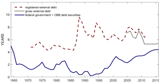
The strategy to sustain growth through external borrowing was successful in the first few years, as the accumulation of public debt was compatible with the maintenance of economic growth at high rates. Continuity of this process, however, relied on other factors: on the growth of private wealth, on the wealth holders’ confidence in the capability of the public sector to service its debt, and on the use that was ultimately being made of the savings captured by the government. In the second half of the decade, GDP growth declined sharply, inflation doubled, and controlling the growth of public-sector financial needs became increasingly difficult. In the 1973–1980 subperiod, the average maturity of the federal government debt securities reached its peak in 1975 (figure 10), but the share of nonindexed bonds kept growing (figure11) until the end of the decade, as interest rates began to rise in 1976 following the abandonment of the interest rate ceilings, which had prevailed until September 1976.
The first year of President General Jo˜ao Figueiredo’s term, 1979, started with a reduction in the real value of public bond debt due to two effects. The first was the decline in real interest rates due to the decline in nominal interest rates promoted by Planning Minister Antˆonio Delfim Netto in an attempt to stimulate economic activity, which reduced the attractiveness of the debt.21 The second effect was the increase in
exchange rate uncertainty related to the second oil crisis. Figure 12 shows how interest rates were kept consistently below inflation rates between 1979 and 1981. Both factors led to a decrease in the stock of public domestic debt (figure3) and an increase in the fraction of government debt securities that are indexed to inflation (figure 11). The policies implemented by Delfim Netto, mainly low nominal interest rates and the corresponding increase in the growth rate of the monetary base, had the effect of significantly increasing inflation, from around 50 percent in 1979 to over 100 percent in 1980.
3.2
1981–1994: no growth with high macroeconomic instability
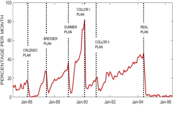
If the previous subperiod was characterized by the number of national development plans that were implemented, the subperiod 1981–1994 is famous for its number of stabi-lization plans, some of which are indicated in figure13, and by severe balance of payments
20The government did not have control over the budget of its SOEs. Given the deterioration of their
accounts and trying to control that process, the government created the Secretary of Coordination and Governance of State-Owned Enterprises (SEST) in 1979.
21Delfim Netto replaced Mario Henrique Simonsen in August 1979 as the de facto manager of the
problems.22 In this section, we discuss Brazil’s balance of payments crisis and provide a
description of its stabilization plans during the 1980s and early 1990s, focusing on their main points and reasons for their failures, and trying to find out the most important differences between them and the ultimately successful plan, the Real Plan.
Even though inflation was increasing to rates above 100 percent per year, in the first half of the 1980s, the greater concern was to reduce external imbalances rather than reduce inflation. In 1981 and 1982, the main objective of Brazil’s macroeconomic policy was to reduce the need for foreign capital. Figure14 shows the current account balance, trade balance, and net interest income. We can observe the increasing cost of interest payments on external debt and the trade balance reversal (from deficit to surplus) in those years. There was a large devaluation of the real exchange rate (figure 15), and real GDP per capita contracted sharply.23 In 1982, Brazil entered a sequence of episodes
in which it accumulated arrears on interest payments of its external debt, illustrated in figure 16, that would end only in 1994.24 These facts account for the drop in external
debt financing and the rise in interest payments on external debt reported in table 1, subperiod 1981–1994. During that period, we also observed the nationalization of the external debt. Foreign debtors would pay the Central Bank of Brazil in domestic currency, and the central bank would retain those funds in the name of the creditors. Any gains or losses resulting from the debt negotiations regarding write-offs and so on would be captured by the central bank. In addition, new foreign debt would be deposited at the central bank, which would then lend those funds to local debtors in local currency. As a result, a large fraction of the external debt became concentrated in the central bank’s balance sheet up to 1994, as figure17 illustrates.
While the government’s attention was focused on the balance of payments crisis, inflation kept increasing. It was only in 1986 that the sequence of stabilization plans began. But before moving to the discussion about each stabilization plan in detail, it is important to put into perspective what was considered to be the cause of high inflation at that time. The first plans were based on the idea that inflation inertia due to the highly indexed economy was the essence of the inflationary process, and breaking that inertia should be the main focus of the stabilization plan. These plans had a neutral shock of freezing prices as one of their main characteristics. However, the staggering of wages and other prices under very high inflation was an extra obstacle to that strategy. At the moment that a price freeze to stop inflation was introduced, agents with similar average real wages would have different real wages depending on when the last adjustment was set. Since inflation was supposed to decrease substantially after the plan, the differences in real
22For thorough analyses of that period, we refer to Carneiro and Modiano (2014), Modiano (2014),
and Abreu and Werneck (2014).
23Under our convention for the real exchange rate, a real depreciation happens when the real exchange
rate increases.
wages at the moment of the plan would prompt losers to claim rights to be compensated, while the winners would not complain. If the losers were compensated, that would reignite the inflation spiral. To avoid that problem, a conversion table was always mandated at the beginning of each plan, aiming at keeping, in the new low inflationary environment, the same average real wage that had prevailed under the previous high inflationary period.25
An alternative and more standard orthodox theory considers the persistent and large fiscal deficits as the main cause of the inflationary process, since the government had to increase the growth rate of the monetary base to raise seigniorage revenues to finance those deficits. We discuss both theories in section 4. As we will see, from the first to the last plan, there was less emphasis on the heterodox part of the plan, which comprised price freezes, and more emphasis on the orthodox part. Fiscal and monetary policies became a major component of the latter plans while maintaining a device to synchronize the adjustment of nominal variables to avoid threatening the new low inflation level.
Cruzado Plan: In February 1986, the government implemented the Cruzado Plan. As what became standard in most Brazilian stabilization plans, the first rule was to change the currency, in that case from cruzeiro to cruzado, which meant cutting three zeros. Prices were frozen, and any indexation clauses for periods shorter than one year were forbidden.26 Wages were converted into cruzados based on the average purchasing power of the last six months but could be readjusted every time inflation hit 20 percent or during the annual readjustment cycle. Moreover, unemployment benefits were introduced, and the minimum wage was raised by 8 percent in real terms. The exchange rate regime also changed, with the domestic currency now pegged to the US dollar. Fiscal and monetary policies were put under the discretion of the policymakers, but there was an important change: the end of the Conta de Movimento between the central bank and the Bank of Brazil. In practice, however, that only took place after 1988 because another account between the central bank and Bank of Brazil, Conta de Suprimentos Especiais, replaced Conta de Movimento until its extinction in 1988 (see section 4). Another important measure was the creation of the National Treasury Secretariat, which would take control over both the administration of the domestic public debt and the government budget.27
At first, the Cruzado Plan was very successful in reducing inflation. The average
25The change of currency allowed for reductions of those wages that had recently been adjusted, in
order to keep the same average real wage. Without the change of currency, the reduction in nominal wages would not be possible, since nominal wage reductions are not allowed by Brazilian law.
26For fixed rate contracts, a schedule for interest rate conversion was set. It was assumed that all
nominal interest rates were based on the inflation expectation of 0.45 percent a day (210 percent a year), which had been the average daily inflation in 1985–1986. The real rate, then, was the (new) nominal rate in the new currency (cruzado), since the new expected inflation (at least for the government) was zero. For the variable interest rate contracts, which prescribed a nominal rate equal to the sum of the monetary correction and variable (real) interest rates, the new nominal rates in cruzados were set to be the ones above the monetary correction before the plan.
27Before that, the Central Bank of Brazil managed both the domestic and external public debt, which
monthly inflation from March to July of 1986 was 0.9 percent (11 percent per year). Moreover, the claim to freeze prices had a civic impact since the population was encour-aged to “audit” prices; but that led to overheating. Sales increased 23 percent in the first six months of 1986 compared to the first six months of 1985, and real wages increased 14 percent from March to September of 1986 (figure 18). One story that is consistent with such evidence is that even though prices were not allowed to change, equilibrium prices were increasing, which produced overheating since posted prices were too low. Therefore, production increased to meet the higher demand in the beginning, but then production decreased and stores started to run out of stock. Meanwhile, the Central Bank of Brazil tried to keep interest rates low to induce low expectations. One huge imbalance was the inconsistency of the plan for inflation and the monetary base: the monetary base was increasing much faster than inflation itself.
In July 1986, the government implemented a timid fiscal package, Cruzadinho, focus-ing on increasfocus-ing government revenues. But in reality,Cruzadinhohad the opposite result of what policymakers expected. Expecting prices to be allowed to change again, demand increased and the overheating problem became even more dramatic. Inflation remained low, but it was not truly representative because products were scarce. Because of the high demand, imports kept increasing while exports declined (figure 19), thereby exac-erbating the trade deficit. A rumor of a large devaluation in the near future reinforced that pattern. This expectation lead to a postponement of exports and an acceleration of imports, which increased the problems with the balance of payments.28 Facing all these
challenges, in November 1986, the government opted for a fiscal plan, Cruzado II, trying to increase revenues through the readjustment of some public prices and some indirect taxes, which led to a high inflationary shock. Once again, the environment was one of high inflation (17 percent per month in January 1987). Meanwhile, the external crisis was just getting worse. In February 1987, the government suspended interest payments on external debt for an indeterminate amount of time (figure 16). The idea was to stop the losses of international reserves and to start a new phase of the renegotiation of the debt with the support of the population.
Bresser Plan: In July 1987, the government implemented the Bresser Plan, named after Finance Minister Luiz Carlos Bresser-Pereira. It was presented as a hybrid plan, with fiscal and monetary policies as well as aspects to deal with inflation inertia. As in the Cruzado Plan, prices were frozen. As usual, the moment in which the price freeze took place was important because the relative prices would remain stuck and possibly off-equilibrium. Trying to get a better result than the Cruzado Plan in this aspect, after the price freeze there was an increase in the prices of public services and some
28The government kept the mini-devaluations based on an indicator of the exchange rate–wage
(crawling-peg) ratio. However, this same indicator was suggesting that the exchange rate was appreci-ated.
administered prices to correct for misalignments in relative prices. The extinction of the automatic trigger in wage resetting if inflation surpassed a 20 percent threshold was also perceived as another improvement. But the economic team created another kind of wage indexation, the URP (Price Reference Unit), in which in each quarter the government would specify the readjustment for the next three months based on the average inflation of the period. This would keep a monthly readjustment, but a gap would remain between the readjustment and current inflation. In contrast to the Cruzado Plan, monetary and fiscal policies were active. Real interest rates remained positive in the short term. In the fiscal policy arena, the government aimed to reduce the operational deficit from the expected 6.7 to 3.5 percent of GDP.29 The plan did not address (or seek to deal with) the consequences of the previous default with creditors. Another interesting aspect of this plan is that it did not target zero inflation, but was meant to be just a deflationary shock.
Bresser-Pereira’s main purpose was to introduce a fiscal reform to reduce inflation. However, the reform was not successful. In 1987, the deficit was much higher than promised. Unlike the Cruzado Plan, which had popular support, the Bresser Plan was not popular, and in February 1988, some liberalization of prices took place, reducing the effectiveness of the price freeze. A third problem of the plan was that it led to a fall in gross fixed capital formation.
After Minister Bresser-Pereira left, Ma´ılson da N´obrega, the second in command, took his position. In January 1988, the government adopted an economic policy referred to as theFeij˜ao-com-Arroz policy, which can be translated to English as the “Black-Beans-and-Rice” policy.30 Instead of freezing prices, its target was merely to keep inflation at
15 percent per month. The deficit was expected to reach 7 to 8 percent of GDP in 1988, and there was a temporary freeze of public-sector wages to reduce it.
At first, this policy succeeded in avoiding an inflationary explosion, and the fiscal stance improved. The default on external debt was suspended, and the government started negotiations with external creditors. However, inflation started rising again, and the target of 15 percent per month was not achieved in the second quarter of 1988.
In October 1988, a new constitution was enacted. The new constitution increased fiscal expenditures, reduced the flexibility of expenditure switching between fiscal ac-counts, and substantially increased labor costs. It did so by increasing expenditures and increasing the transfers from the central government to states without transferring the corresponding responsibilities, which induced an increase in the deficit of the central
gov-29At the time, the government used the public-sector borrowing requirement as a measure of the
nominal deficit. However, nominal deficits were very high because of the monetary correction of the value of the debt. In order to overcome that, the operational deficit was adopted as the main deficit measure, which included only the nominal value of real interest payments. See appendixC.
30The policy name reflects the meaning of black beans and rice in Brazilian culture. It is the dish that
Brazilians eat every day. It is considered to be neither very interesting nor complicated, but it does the job of providing a healthy meal.
ernment. To put this into perspective, 92 percent of the revenues were earmarked; that is, revenues from different sources were dedicated to specific programs or purposes (or both), reducing the flexibility of fiscal policies. In addition, the new constitution reduced the standard weekly working time from forty-eight to forty-four hours and increased the cost of overtime.
Summer Plan: The government implemented the Summer Plan in January 1989. Again, it was a hybrid plan, but the debate on the need for changes in fiscal and monetary policies was increasing. Like the previous plans, it included a component of price freezing as well as the adoption of a nominal anchor. In this case, a fixed exchange rate (1 cruzado novo = 1,000 cruzados = US$1) was implemented for an indefinite time. Moreover, an attempt was made to end inflation indexation. On the fiscal and monetary side, the plan was to adopt a tight monetary policy and to fight inflation by controlling the public deficit. It intended to control expenditures and increase revenues through the privatization of publicly owned assets and a reduction in the wage bill of the public sector.
Overall, the plan seemed to incorporate everything that was missing in the previous plans. Although it kept a heterodox flavor, it was mostly an orthodox plan aiming to reduce subsidies, close public firms, and fire public employees, with a deindexation plan that was sort of a small default. However, the government did not have the political power to carry it through. Without Congress, privatizations and other unpopular measures, such as the closing of public firms, were canceled. In the end, the reforms were not implemented. Moreover, the tight monetary policy put interest rates at high levels and increased the fiscal deficit of the government. With low credibility and a reform that did not go through, inflation accelerated, and the Summer Plan also failed.
The 1980s ended with inflation rates of about 70 percent a month and with almost 100 percent of the federal bond debt being rolled over in the form of zero-duration bonds.31
This state of affairs reflected not only the extremely high uncertainty regarding inflation and interest rates but also the fear of an explicit default of the public debt by the incoming administration, headed by President Fernando Collor de Mello. At the time, the credit risk of the public securities was clouded with widespread suspicion, which was indeed validated by the new administration’s actions. Collor de Mello was elected president of Brazil after twenty-nine years of either indirect or undemocratic elections. The very day he took office, he launched the first Collor Plan.
Collor Plan I: In March 1990, the government launched the Collor Plan I. Prices and wages were frozen. The plan recognized that a reduction in deficits was necessary to end the hyperinflation, and it implemented both temporary and permanent fiscal policies. Among the temporary measures were the establishment of a tax on financial
in-31Zero-duration bonds are bonds that pay ex post the accrual of daily overnight interest rates.
There-fore, the price of these bonds is insensitive to interest rate changes. It was a way to separate interest rate risk from maturity risk, thereby somewhat lengthening the very short-term public debt.
termediation and the suspension of tax incentives. But the permanent policies were more important. An effort was made to reduce fiscal evasion (one of the president’s trade-marks during the presidential campaign) and increase taxes. Other major components included privatizations and an administrative reform. However, that plan became famous for its (controversial) monetary policy. In an attempt to reduce the money supply, the government confiscated deposits in both transaction and savings accounts for a period of eighteen months.32 Those resources amounted to 80 percent of bank deposits and financial investments, which would be held at the Central Bank of Brazil and invested in federal government bonds. These resources were remunerated while they were kept at the central bank, but their rates of return were decided by the government itself and therefore were subject to partial defaults.
Following the plan’s implementation, monetary aggregates fell sharply, especially the higher ones (figure20), and real GDP per capita contracted by 5.7 percent in 1990. This reduction in liquidity, however, was not sufficient to control inflation. Regarding the fiscal reform, the threatening behavior of the government toward the public-sector employees made the reform very unpopular. The plan encountered a lot of resistance, and in the end, it could not deliver on what it had promised. While some privatizations succeeded, most of its reforms were short-lived.
Collor Plan II: In January 1991, the same government implemented the Collor Plan II. Just like the previous one, it planned to reduce government expenditures by firing civil servants and closing public services. It also proposed the privatization of state-owned enterprises. As usual, the plan included some price freezes. Wages were converted by a twelve-month average, a new tablita was adopted based on the assumption that inflation would fall to zero, and the plan put an end to indexation.33 Not entirely related to the
fight against inflation, this plan had a motif that Brazil had to improve the quality of its products. In the words of the president, Brazil was producing horse-drawn coaches instead of cars. To achieve that goal, the government opened the Brazilian economy to foreign competition and privatized state-owned firms.
Following the plan’s implementation, the country experienced a recession. But it re-covered afterward, and this recovery is usually attributed to enhanced competition in the economy. Inflation ended up rising again, but this plan did make two important perma-nent changes. First, it opened up the Brazilian economy and expanded trade, reversing the previous trend (figure19). Second, it increased productivity. In the beginning of 1992, when expectations of accelerated inflation did not materialize, the effects of the recovery in investors’ confidence started to show up in public debt markets. Those expectations had been based on the combination of price liberalization, corrections of public tariffs,
32The government confiscated the amounts exceeding $50,000 cruzados novos. The resources actually
became available before the eighteen-month period, as figure20shows.
and the devaluation that followed the floating of the exchange rate in October 1991, in face of the strong monetization of the hijacked assets during Collor Plan I.34 The return
of investors’ confidence is also confirmed by the recovery of foreign exchange reserves after 1992.
Following the high political turbulence that characterized the months preceding the impeachment of President Collor de Mello (October 2, 1992), the beginning of Itamar Franco’s presidency was marked by high uncertainty concerning economic policy. Propos-als of another moratorium, and even repudiation of the public debt, were constantly in the press. It was only after the president nominated Fernando Henrique Cardoso, his fourth minister of finance in less than six months, that the recovered confidence materialized in higher external reserves.
Real Plan: In February 1994, the government launched its last stabilization plan, the Real Plan, which would finally put an end to the hyperinflation. The plan that conquered Brazilian inflation did not have the blessing of the IMF, an always troubled relationship in the previous decades. The plan’s concepts were different from the previous ones: it aimed to reduce deficits, modernize firms, and reduce the distortions that arose from previous price freezes. An important difference from previous plans is that it was planned in advance, with several measures being taken before its official announcement. Its first stage started in June 1993, when the government launched the Programa de A¸c˜ao Imediata (Program for Immediate Action), designed to focus on fiscal imbalances that would arise when the seigniorage revenues fell.35 It included an increase in existing
tax rates, such as income tax, the creation of new taxes, such as the tax on financial intermediation, and the renegotiation of subnational government debt in an attempt to control the deficits of subnational governments.36 Another fiscal adjustment came in the
beginning of 1994, with theFundo Social de Emergˆencia (Emergency Social Fund), a way to suspend part of the earmarked revenues of states and municipalities, providing more flexibility in the government budget. On the monetary side, a clearly stated intention to limit issuances of the new currency led to the adoption of a high interest rate policy and high reserve requirement ratios (100 percent reserve requirements on new deposits after July 1, 1994). In addition, the plan included changes in the institutional framework in which the central bank operated, such as the transfer of management of the external debt to the National Treasury Secretariat and the reduction of the size and duties of the National Monetary Council. Section 4 discusses those changes in more detail. On
34The recovery of the stock of public debt in the portfolio of the private sector was a clear demonstration
that asset holders were willing to return to business as usual in spite of the disruptions of repeated interventions that had been made in the rules of indexation and the liquidity of public securities during the previous twelve years. One should bear in mind that the majority of economic analysts at the time were forecasting that the government would never again be able to place new debt.
35The program was announced in June 1993, but many of the reforms were implemented later in that
year or even in 1994.
top of all these measures, the government also reached an agreement on its external debt renegotiations under the Brady Plan, and in March 1994 its defaulted debt was securitized and the country regained access to international capital markets.37
The Real Plan did not involve price freezes itself, but it was able to solve the problems of staggered wages and prices. Actually, this was considered the most controversial aspect of the plan but ended up being very successful. The creation of a new unit of account, the URV—Unidade Real de Valor (Unit of Real Value)—aimed at establishing a parallel unit of value to the cruzeiro real, the inflated currency. The idea was to make the unit temporary. Prices were quoted in both URVs and cruzeiros reais, but payments had to be made exclusively in cruzeiros reais. The URV worked like a shadow currency that had its parity to cruzeiro real constantly adjusted, since it was one-to-one with the dollar. Therefore, a conversion rate of the URV/cruzeiro novo (the old currency) was set every day, and many conversions were left to free negotiation between economic agents, with the government having more interference in oligopolized prices. That would allow agents to observe the low inflation of the parallel currency, therefore breaking the expectations of high inflation once the currency was changed. The URV was created in February 1994 when the Real Plan was officially launched, and in May 1994 the government announced that the real would become the new currency in July 1994. The government kept its plan, and the URV was extinguished on July 1, 1994, when it was converted to the new currency, the real, with the parity being 1 dollar = 1 real = 1 URV = 2,750 cruzeiros reais, and the adoption of a crawling-peg regime followed.
After the currency conversion was implemented, inflation rates fell significantly, and the hyperinflation period in Brazil came to an end. Figure21illustrates how the increas-ing primary surplus since 1993 allowed the government to reduce its seigniorage revenues after the Real Plan was implemented. The drop in seigniorage revenues was associated with a reduction in both inflation and money growth rates. In table3we use the monthly data to compute the government budget constraint around the time the Real Plan was implemented. Note that while the primary surplus increased in May/93–May/94, the government was able to accumulate foreign reserves by 6.3 percent of GDP (which ex-plains the negative 6.3 percent of GDP relative to net external debt in table 3). Then, between May/93–May/94 and May/94–May/95, seigniorage revenues fell from an average of 2.7 percent to only 0.7 percent of GDP, and that was possible because of the increase in primary surplus, from 2.8 to 4.0 percent of GDP, as a result of the fiscal measures described above. However, in May/95–May/96, after inflation was under control and seigniorage revenues fell, the government showed a deterioration in its primary balance that would be reversed in the subsequent years. That fiscal deterioration was financed through domestic debt issuance, which shows that the credibility of the reforms played an important role, as it allowed the government to keep seigniorage revenues at low levels.
In addition, the increase in real money balances following the Real Plan also contributed to increasing the financing options of the government (figure 22). Lastly, Brazil started to accumulate external debt again after 1994, but that was done by the private sector (or by public entities that were not included in the fiscal and debt statistics), which borrowed from abroad and, concurrently, financed the government. That accounts for the current account deficits after 1994 (figure 14), explained by lower trade balances as a result of increasing imports (figure 19).
Here, it is important to mention that the analysis above used the official primary deficits plus transfers as the benchmark measure of government primary deficits. We did so because there are large discrepancies in fiscal statistics around the time the Real Plan was implemented.38 If instead we considered only the primary deficits from government
accounts, without thetransfers, we would observe a transition from large primary deficits to large primary surplus upon the implementation of the Real Plan, without the subse-quent deterioration in primary balances mentioned above. We discuss that in appendix
C. We were not able to explain the differences between both series. We chose theprimary deficits plus transfers as our benchmark measure because it is closer to the primary deficit series reported by the Central Bank of Brazil, and it has been the preferred measure by economists that analyzed the fiscal policy in Brazil at that time (e.g., Giambiagi and Alem 2011 and Portugal 2017).
Under our benchmark measure of primary deficits, the fiscal deterioration from May/94– May/95 to May/95–May/96 is usually explained by the increase in wages that resulted from wage negotiations in 1994, and by the Bacha effect, which worked as the reverse of the Olivera-Tanzi effect.39 The reason is that fiscal revenues in Brazil were very well
in-dexed to inflation, but fiscal expenditures were not.40 So the executive branch could, and
indeed did so, cut the real value of expenditures just by disbursing the originally planned nominal amounts with some delay, as higher inflation rates would rapidly erode the real value of those expenditures. Of course, this had the collateral effect of creating large problems, since public hospitals would run out of money at the end of the year, several bridges or roads would stay unfinished for many years, and so on. Guardia (1992) studied the budget for 1990 and 1991 in detail and reported significant differences between total expenditures in the (federal) budget and the actual expenditures. In 1990 and 1991, total expenditures hovered around 63 and 60 percent of the voted expenditures, respectively. Therefore, after inflation was under control, the government had to deal with the large discrepancies between nominal expenditures and revenues in the budget, which could
38One advantage is that it allows us to make the analysis using monthly data because the official fiscal
statistics covering the national public sector are reported at an annual frequency.
39See Bacha (2003) and Tanzi (1977).
40A daily index, the UFIR (Fiscal Reference Unit), was computed based on inflation. Taxes would be
denominated in this indexed unit of account and then translated to the nominal hyperinflated currency on the very day that taxes were paid to the banking system.
explain the temporary deterioration in fiscal balances in the subsequent years.
The success of the Real Plan in conquering the hyperinflation is indisputable, but many discussions have taken place regarding which were the most important points in accounting for it. As is evident, many important changes were taking place around the implementation of the Real Plan, so it is hard to answer that question. One important condition was the availability of foreign financing, as foreign capital inflows resumed after the government reached an agreement with its foreign creditors under the Brady Plan.41 That was the end of a long process of foreign debt rescheduling. Another important factor was the fiscal reform that increased primary surpluses (figure 21). That reform also included other important fiscal measures that, most likely, did not have an immediate impact on government fiscal statistics. Among those measures was the imposition of fiscal constraints on subnational governments, seen as an important achievement of the Real Plan. The deficits of the subnational governments became a big issue in the 1980s and 1990s, and many attempts were made, often including bailouts, to solve that issue. In 1989, for example, a debt renegotiation with the state governments took place, and only two years before the government had renegotiated the debt of ten state banks. The state banks, in particular, were constantly used to finance subnational government deficits. Many of them actually operated with negative reserves, which ultimately pressured the central bank to expand the monetary base (see section4.1). In 1993, the reforms enabled the federal government to use the fiscal revenues of subnational governments as debt guarantees and also forbid the state banks from making new loans to their respective state governments. That was the beginning of a sequence of reforms that would culminate in the implementation of the Fiscal Responsibility Law in 2000. Finally, the tightness of monetary policy was an important characteristic of the Real Plan, and it still characterizes monetary policy to this day.
3.3
1995–2016: moderate growth with higher stability
The last subperiod of our analysis represents the period of lowest inflation in Brazilian history. Inflation rates averaged only 8 percent per year, accompanied by the adoption of active fiscal and monetary policy rules. Economic growth resumed, but at moderate rates. Real GDP per capita grew 1.2 percent per year on average. We also observed the process of fiscal consolidation, with primary surpluses in 1995–2002 and 2003–2011 averaging 2.3 and 2.8 percent of GDP, respectively (row 9, table 1). Despite all those advancements, the country experienced a big shift in its economic policy at the onset of the international financial crisis in 2008–2009, which eventually culminated in a rapid
41The capital inflows were a main factor in the expansion of the interest-bearing public debt, as the
Central Bank of Brazil conducted massive sterilized purchases of foreign exchange. In 1993, so much capital was flowing into Brazil that the government implemented controls on capital inflows (Carvalho and Garcia 2008).
deterioration of its fiscal balances and a deep recession in recent years. These events have raised concerns about the capability of the government to maintain a low-inflation regime in the future.42
3.3.1 1995–2002
The years following the implementation of the Real Plan represented a consolidation of the reforms that had begun in the previous subperiod. The government kept the pri-vatization process and promoted both fiscal and banking reforms. Part of these reforms were possible only because of the success of the Real Plan in conquering the hyperinfla-tion, which gave the government the political support to push its agenda of reforms. The value the public bestowed on the new low-inflation scenario became clear in the follow-ing presidential elections. Fernando Henrique Cardoso, the finance minister durfollow-ing the elaboration of the Real Plan, was elected president of Brazil in the first round, not only in the presidential elections of 1994 but again in the 1998 elections.43
The low-inflation regime, however, also brought some challenges. For example, a banking crisis followed the Real Plan, during which some private and state-owned banks failed. One of the reasons for the failure was that the fall in inflation led to a fall in seigniorage-like revenues (the float) that were partially captured by these banks. Here is an example of how this mechanism works. The Central Bank of Brazil increases the monetary base by $1,000 reais by depositing that amount in the account that holds the bank reserves. Assuming that the banks have no incentives to hold any voluntary reserves, the banking system lends the $1,000 reais to the public. The public borrows that amount, and after spending it, the $1,000 reais return to the banks as deposits. Assuming that the reserve requirement ratio is, for example, 10 percent, the banks keep $100 reais as reserves and now have $900 reais left to lend to the public again. Then the public borrows that amount, and after spending it, the $900 reais return to the banking system as deposits again. The banking system holds $90 reais as reserves and lends the rest. That process continues indefinitely, and the increase in the amount of deposits converges to $10,000 reais (= $1,000 + (1−10%)×$1,000 + (1−10%)2 ×$1,000 + . . .), which represents ten times (the inverse of the reserve requirement ratio) the initial increase in the monetary base. The ratio of deposits to bank reserves in Brazil is illustrated in figure 23. Finally, given that banks charge interest when lending money to the public, and that deposits are usually not remunerated, that process represents an increase in the revenues of the banking system. So, overall, in order for inflation to fall, the Central Bank of Brazil must
42For thorough analyses of that period, we refer to Werneck (2014a,b).
43According to the constitution of 1988, the president is elected by a majority voting in a two-round
system. If a presidential candidate receives more than 50 percent of the valid votes in the first round, that is, after the exclusion of blank and null votes, then the candidate is elected president without a second round. So far, no other presidential candidate besides Fernando Henrique Cardoso has been elected in the first round after the constitution of 1988 was enacted. Voting is mandatory in Brazil.
make fewer such increases to the monetary base and thus must collect fewer revenues, as we have just described. That decrease in revenues hurt the balance sheets of banks and, all else equal, contributed to the banking crisis.
Besides the banking crisis, the government also faced turbulence in international cap-ital markets. The first one was the 1997 Asian financial crisis, which was immediately followed by the 1998 Russian financial crisis. After the latter, there was a speculative attack on the real, and the Central Bank of Brazil experienced a fast deterioration of its international reserves (figure 24). The IMF stepped in, but the situation was such that the central bank could no longer hold the crawling-peg regime, and in January 1999, a floating exchange rate regime was adopted. This change also culminated in the replacement of the governor of the central bank, but not of the finance minister.44
In March 1999, following the adoption of the floating exchange rate regime, Brazil adopted an inflation-targeting regime, an arrangement that holds to this day. Concur-rently, the government started to announce fiscal policy targets and took important mea-sures to improve the conduction of its fiscal policy. One important step in that process was the Fiscal Responsibility Law, enacted in 2000, which imposed rigid fiscal constraints on both federal and subnational governments. Those measures led to fiscal surpluses, as illustrated in figure 9.
However, the government faced another deterioration in the external scenario in 2001, with the recession in the United States and the fall of the Argentine peso. To make matters worse, the country also experienced a major energy crisis. It resulted from the poor management of its infrastructure, and the government ended up imposing mandatory rationing of electricity. The government lost its popularity, and during the presidential campaigns of the 2002 elections, the stability of Brazil’s macroeconomic policy was put to the test. The polls indicated that Luiz In´acio Lula da Silva, “Lula,” would be the new president, and that led to an episode of current account reversal (figure 14), with a large devaluation of the real exchange rate (figure 15) and a sharp increase in the interest rates of government debt securities, in both the domestic and external debt markets. The reason behind this new episode is that the leading candidate had advocated for a debt renegotiation of both domestic and external debt in the past, indicating the possibility of an outright default. Under the adverse scenario, the IMF stepped in again, its last intervention in Brazil. Lula ended up announcing that he would keep the main macroeconomic policies that the previous government had implemented. Once elected, he kept his promise, and the financial markets returned to normality.
3.3.2 2003–2011
The years following the election of President Lula were characterized by a favorable external scenario, with a worldwide boom in commodity prices. In particular, the period between 2004 and 2008 had the best economic outcomes of the 1960–2016 period. It was characterized by fiscal surpluses, high growth rates of real GDP per capita, current account surpluses, an expansion of international trade, a reduction of the public exter-nal debt and the accumulation of internatioexter-nal reserves, and the consolidation of the inflation-targeting regime that had been adopted in 1999. In addition, the government implemented large conditional cash transfer programs, such as the social welfare program Bolsa Fam´ılia, which led to big improvements in income inequality in the fight against poverty.
Nevertheless, following Lula’s reelection in 2006, the government shifted its macroe-conomic policy toward a larger intervention of the state in the economy, which would eventually lead to a deterioration in fiscal balances. In 2007, for example, the govern-ment launched the Growth Acceleration Program (PAC), a major infrastructure program consisting of investment projects and policies that aimed at boosting economic growth. Through BNDES, Brazil’s development bank, the government began to invest heavily in large national companies in an attempt to increase its competitiveness in the global market. And through the now state-controlled mixed-capital oil company Petrobras, the government promoted large investments in the exploration of oil in the pre-salt layer, which had recently been discovered. As expected, some of these policies represented the expansion of fiscal deficits, but since neither BNDES nor Petrobras was included in the public-sector fiscal statistics in that time, they did not show up in the official statistics. In fact, in those years the government started to implement budget maneuvers to artificially inflate its primary surplus to meet the fiscal policy targets, which makes the assessment of the actual fiscal deficit figures even harder for that period. That effort became popularly known as contabilidade criativa (creative accounting).
With the global financial crisis in 2008–2009, the government started to push those policies even further, seeking to implement a countercyclical policy that would prevent the country from going through a major recession. Initially, the policy seemed to be very successful, as real GDP per capita grew 6.2 percent in 2010. However, it did not last for long.
3.3.3 2012–2016
In 2012, the economy was already showing signs of exhaustion, with annual growth rates of real GDP per capita decelerating to only 1 percent. The drop in commodity prices made the situation even worse. The fiscal deterioration accelerated, and the use of contabilidade criativa to hide deficit figures became even more pronounced. The
govern-ment was now also intervening in SOEs in an attempt to manage inflation through the control of administered prices; that is, the government maintained low prices for goods and services (e.g., fuel and electricity) that were sold by SOEs, even though the other prices in the economy were increasing. The main reason for this intervention is that the government did not want to bear the political burden of reporting higher inflation rates, since it was the government itself that pressured the central bank to reduce nominal interest rates in the first place.
Further, the government also used its public banks (as well as private banks) to hide its deficits. Here is one way that it did so. The government instructed the public banks to pay social security pensions to the public, but then the government never reimbursed the public banks for the full value of those payments. Hence, the public banks registered losses that should have been counted as deficits of the government.
Brazil was now back to a scenario in which the government used public banks and SOEs to hide its deficits while economic growth kept decreasing. These fiscal maneuvers became popularly known as pedaladas fiscais and eventually led to the impeachment of former president Dilma Rousseff in 2015, who had replaced Lula in 2010 and was reelected in 2014.
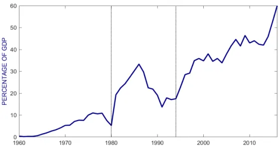
In 2015 and 2016, real GDP per capita decreased by 4.6 and 2.7 percent, respectively, and fiscal deficits reached levels of around 7 percent of GDP in 2016. The fiscal situation proved to be worse than previously expected. The previous government avoided tackling the reforms that would lead to a fiscal consolidation, such as the reforms to the pension system, and, at the time of this writing, the outstanding question is whether the next president can resolve the current precarious fiscal situation. As figure 3 shows, public domestic debt is now at record levels, and previous fiscal adjustments were implemented through higher public expenditures and even higher public revenues. But the tax burden in Brazil is already very high, imposing an extra constraint on the capability of the government to raise more revenues.
With this history in mind, we now turn to discussing why inflation rates were so persistently high before the implementation of the Real Plan.
4
Weak institutions, deficits, and inflation inertia
4.1
Weak institutions that provided indirect access to the
print-ing press
One of the most striking features of Brazilian monetary and fiscal history is its long period of high inflation pre-1994. Figure 5shows that inflation rates were closely related to the growth rates of the monetary base and to seigniorage revenues. We argue that the high degree of passiveness in monetary policy due to a weak institutional arrangement,