Audio classification using attention-augmented convolutional neural network

Northumbria Research Link

Citation: Wu, Yu, Mao, Hua and Yi, Zhang (2018) Audio classification using attention-augmented

convolutional neural network. Knowledge-Based Systems, 161. pp. 90-100. ISSN 0950-7051

Published by: Elsevier

URL: http://dx.doi.org/10.1016/j.knosys.2018.07.033 <http://dx.doi.org/10.1016/j.knosys.2018.07.033>

This version was downloaded from Northumbria Research Link: http://nrl.northumbria.ac.uk/39658/

Northumbria University has developed Northumbria Research Link (NRL) to enable users to access

the University’s research output. Copyright © and moral rights for items on NRL are retained by the

individual author(s) and/or other copyright owners. Single copies of full items can be reproduced,

displayed or performed, and given to third parties in any format or medium for personal research or

study, educational, or not-for-profit purposes without prior permission or charge, provided the authors,

title and full bibliographic details are given, as well as a hyperlink and/or URL to the original metadata

page. The content must not be changed in any way. Full items must not be sold commercially in any

format or medium without formal permission of the copyright holder. The full policy is available online:

http://nrl.northumbria.ac.uk/pol

i cies.html

This document may differ from the final, published version of the research and has been made

available online in accordance with publisher policies. To read and/or cite from the published version

of the research, please visit the publisher’s website (a subscription may be required.)

Audio classi

fi

cation using attention-augmented convolutional neural

network

Yu Wu, Hua Mao

⁎

, Zhang Yi

Machine Intelligence Lab, College of Computer Science, Sichuan University, Chengdu 610065, China

A R T I C L E I N F O

Keywords: Audio classification Spectrograms

Convolutional neural networks Attention mechanism

A B S T R A C T

Audio classification, as a set of important and challenging tasks, groups speech signals according to speakers’

identities, accents, and emotional states. Due to the high dimensionality of the audio data, task-specific hand-crafted features extraction is always required and regarded cumbersome for various audio classification tasks. More importantly, the inherent relationship among features has not been fully exploited. In this paper, the original speech signal isfirst represented as spectrogram and later be split along the frequency domain to form frequency-distributed spectrogram. This paper proposes a task-independent model, called FreqCNN, to auto-maticly extract distinctive features from each frequency band by using convolutional kernels. Further more, an attention mechanism is introduced to systematically enhance the features from certain frequency bands. The proposed FreqCNN is evaluated on three publicly available speech databases thorough three independent classification tasks. The obtained results demonstrate superior performance over the state-of-the-art.

1. Introduction

Audio classification technologies distinguish audio data by the dif-ferences of emotion, accents, speakers’identities, and other factors. Effective audio classification tasks can also contribute to the perfor-mance of other tasks, e.g., speech-to-speech translation and automatic speech recognition. For instance, Akagi et al. [1]translated spoken utterances from one language into another by taking into account emotional states in sounds, which enables their model to deal with non-linguistic information and makes a translation system practical. Hansen and Liu[2]improved the generalization and robustness of their speech recognition system by also detecting accent-related variation in speech signals. Intuitively, by considering the variety of dialects, accents, and emotions in speech signals, better performance could be expected in human-machine speech communication tasks.

Because of the high dimensionality of the original audio data, most audio classification are based on the extracted low-dimensional fea-tures. Spectrograms are considered to capture comparatively complete energy, frequency, and time information from the original audio signal

[3]. However, spectrograms are still considered high-dimensional for traditional classifiers such as support vector machines. To further re-duce the dimensions of the input space, the feature extraction of mel-frequency cepstral coefficients (MFCCs) and the linear prediction cep-strum coefficient (LPCC) are widely used in many studies[4,5]. These

features are hand-engineered because the corresponding parameters need to be predefined based on expert knowledge. Moreover, these predefined feature sets are designed for specific tasks and often fail to generalize to other ones[6,7]. These difficulties in audio classification

research motivate us to find a general solution for automatically learning different features from high-dimensional spectrograms for the corresponding tasks.

Recently, deep neural networks (DNNs) have proved to have an excellent ability to automatically learn salient feature representations from high-dimensional input data[8], as a result of their outstanding performance in many areas[9,10]. The deep architecture in DNNs is a set of non-linear activation functions that enables the network to ef-fectively model complex nonlinear mappings from input to output[11]. Convolutional neural networks (CNNs), which are a type of DNNs, have been popular in pattern recognition[12,13]. A CNN consists of inter-leaved convolutional layers and pooling layers. The former layers uti-lize locally connectedfilters to share weights across the input, which enables translation invariance of the input, and the latter layers are designed to reduce the dimensionality of the data [11]. These con-volutionalfilters also have interpretable time and frequency meanings for audio spectrograms and are able to learn time-frequency feature representations from two dimensions.

Usually, a whole spectrogram is used as the input of a CNN to obtain the global feature representation. To learn more salient features, the

⁎_{Corresponding author.}

E-mail address:[email protected](H. Mao).

spectrogram is split into small frames along the time axis, which is called a time-distributed spectrogram[14,15]. Using these small time-distributed segments of the spectrogram as the input into the CNN, different local features at different time steps are learned. However, spectrograms also represent the distribution of energy along the change of frequency. In many approaches [16,17], frequency-domain only features (e.g., MFCCs) also obtain good results in audio classification tasks, which have proved the importance of frequencies information. Beside, several works have researched the effectiveness of sub-band spectral feature[18–20], which enhanced the representation of speech signals and obtained better robustness in many tasks, such as automatic speech recognition (ASR).

Methods based on the time-distributed spectrogram[14,15]focus on the information of the time domain, while this paper investigates how does the changes in certain frequency bands contribute to thefinal performance of different audio classification. Small segments split along frequencies are called the frequency-distributed spectrogram, and they represent the energy distribution in different frequency intervals. In this way, various features in different frequency intervals can be learned effectively. In some works[21,22], improved DNNs were used in speech related tasks and obtained great performance. Compared with fully-connected DNNs, CNNs have fewer parameters with high non-linearity, which are suitable for smaller dataset. In our work, wefinally apply CNN as the main architecture. Both global features extracted from the whole spectrogram and local features extracted from frequency-dis-tributed sub-spectrograms are learned using different convolutional kernels.

In order to better interpret the features and their relationship from various frequency bands, we further propose attention-augmented convolutional neural networks. The idea of attention comes from the human visual system[23], which prefers to focus on the most relevant piece of data rather than using all available information. In DNNs, ra-ther than concatenate all low-level features into a global representation, the attention mechanism enables salient features to automatically re-ceive more focus as needed [24]. This is especially necessary when there are a lot of features in a DNN. Combing attention with DNNs has been proven to be effective in manyfields, especially computer vision and natural language processing (NLP)[25,26]. In our work, we de-monstrate the efficiency of attention-augmented CNNs in multiple audio classification tasks with state-of-the-art performance.

In this paper, based on frequency-distributed spectrogram, a model called FreqCNN that combines deep CNNs with an attention mechanism is proposed for different audio classification tasks. The proposed FreqCNN is a general model, which automatically learns the relevant feature representation according to auditory categories. The basic idea of FreqCNN is to learn different feature representations from the fre-quency-distributed segments and a whole spectrogram simultaneously and further integrate different features using the attention mechanism. The rest of the paper is organized as follows.Section 2discusses some related work in the audio classificationfield.Section 3presents the preliminaries of spectrograms, original CNNs and the attention mechanism. The details of the proposed FreqCNN are described in

Section 4. InSection 5, a thorough empirical evaluation of FreqCNN is conducted. The conclusion is drawn inSection 6.

2. Related works

Most audio classification studies focus on a specific task in order to achieve good results. For instance, Poria et al.[6]designed two broad kinds of feature sets, short- and long-time based features, to capture the representation of emotions in audio. In[16], they used MFCCs with a support vector machine to improve the performance on two public databases for audio event classification. Mencattini et al.[27]applied 12 different groups of features to learn emotion-relevant information with prominent results. Recently, increasingly more research has ap-plied DNNs to audio classification tasks. In[4], DNNs combined with

transformed MFCCs were used for speaker age classification, which improved the overall recognition accuracy. In speaker recognition, i-vector is a good technique to represent the characteristic of a speaker. Ghahabi and Hernando[28]proposed to combine Deep Belief Networks (DBNs) with i-vector in a speaker verification task, which achieved relative improvements of the recognition performance. In[29], DNN-based gaussian probabilistic linear discriminant analysis system also achieves much improvements in EER values than traditional gaussian methods.

Moreover, several studies using CNNs with spectrograms for audio classification have been conducted recently. In [30], they applied principal component analysis (PCA) whitening to spectrograms to ob-tain the lower-dimensional representation and achieved better perfor-mance by combining with DNNs than traditional well-designed feature sets, i.e., MFCCs, LPCC, and pitch. In contrast to methods using single-input (whole) spectrograms, some studies proposed time-distributed spectrogram combined with CNNs [14,15]. In every time step, one small segment of the whole spectrogram is input to the CNN. Their model can learn the feature representation of audio in a time sequence, demonstrating that distributed spectrograms with CNNs outperforms the whole single-input model.

All these techniques above are restricted to a single audio classifi -cation task, and few studies have focused on a uniform framework to deal with different audio classification problems. Lee et al.[31]applied convolutional deep belief networks (CDBN) to classify audio data. The experiments showed that the feature representation learned by this model can achieve high performance on multiple audio recognition tasks. In[32], they employed DNNs to extract the cepstral features of audio, which outperformed competing methods in two audio classifi -cation tasks. Scardapane et al.[33]provided multiple functional link expansions on three audio classification problems, achieving the best accuracy in two out of three tasks.

3. Preliminaries

In this section, the conversion of audio into spectrograms and CNNs with attention are presented.

3.1. Spectrograms

Spectrograms are a visual representation of audio that resemble natural images. However, there are some noticeable differences be-tween spectrograms and natural images. Natural images can be scaled, rotated, and distorted without losing the underlying image structure, but each pixel in a spectrogram has specific meanings. The spectrogram is depicted as a“fixed”structure that displays the change of frequency along the vertical axis and time along the horizontal axis[3]. It is calculated using the short-time Fourier transform (STFT) on windowed audio frames. In this section, we briefly introduce the conversion of audio into spectrograms. Further details can be found in[3].

The spectrogram of audio is generally organized as a two-dimen-sional matrix as follow:

= ⎡ ⎣ ⎢ ⎢ ⎢ … ⋮ ⋱ ⋮ … ⎤ ⎦ ⎥ ⎥ ⎥ − − S s s s s , M N NM 01 0 (1 1) ( 1) ₍₁₎

whereSdenotes the raw spectrogram.Mdenotes that the original audio signal is segmented into M window frames, and the length of each windowed audio frame isN.

Each spectrogram frame is computed as the estimate of the short-term frequency content for the windowed audio. Let the original audio is denoted as a set of windowed frames (x1_,x2_{, ... ,x}M_{). Each}

∑

= = … = … = − Xkm x e , k 0, 1, , -1, andN m 1, 2, ,M, n N nm i πkn N 0 2 / (2) where xm _{denotes the audio segment at the window with index m.}

Further,

= +

skm (Re X{ km})2 (Im X{ km}) ,2 (3)

whereRe{ · } denotes the real part ofXkmandIm{ · } is the imaginary

part. After all spectrogram frames have been computed, they are con-catenated together to construct spectrogramS.

The visualization of three different emotional states of audio in the form of spectrograms are shown inFig. 1. There is a large difference

among three images in the distribution of energy as frequencies in-crease in the vertical direction. They also indicate the ability to dis-tinguish one audio from another using the energy distribution over the frequencies of the spectrogram.

3.2. Convolutional neural networks (CNNs)

CNNs have been broadly applied in pattern recognition using many typical architectures such as VGG nets[12]or ResNet[13]. In a typical CNN architecture, there are three important parts: convolutional layers, pooling layers, and fully-connected layers.

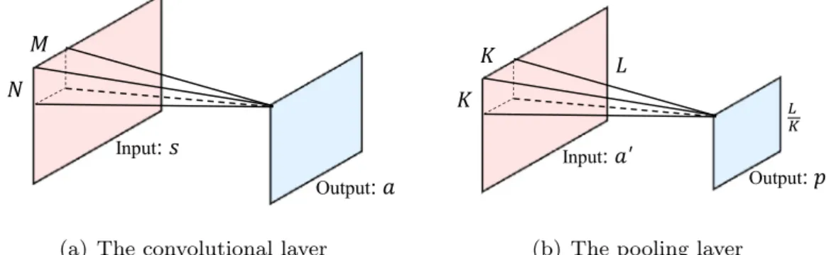
A convolutional layer consists of a set of kernels (also called as fil-ters), each of which has a receptive field. Because of the local con-nectivity and shared filters, convolutional layers can deal with two-dimensional data with translation invariance [11]. For input s, the convolution operation is described by the following equation:

∑ ∑

= ⎛ ⎝ ⎜ + ⎞ ⎠ ⎟ = − = − + + aij f w ·s b , m M n N mn i m j n 0 1 0 1 ( )( ) (4) whereadenotes the feature representation (output after convolution).

w is the weight values of the convolutional kernel, andbis the bias offset. Further,M andN denote the width and height of the kernel, respectively. (i, j) and (m, n) represents the position indices. Functionf

( · ) is the activation function.Fig. 2(a) shows the convolution operation inEq. (4).

The pooling layer is generally applied after several convolutional layers. It provides a form of nonlinear down-sampling of the input and aims to reduce the number of parameters in the network. The output of the pooling can be computed as follows:

= ′

p σ a( ), (5)

wherepanda′denote the output and the input for the pooling layer, respectively. Functionσ( · ) denotes the down-sampling operation over the receptive filed, i.e., maximum or average function. As shown in

Fig. 2(b), the size of inputa′isL×L, and the size of outputpisL × , K

L K

when a receptivefiled of sizek×kis used to reduce it to a single value

via functionσ( · ).

After convolutional and pooling operations, the multiple feature maps are aggregated and used as the input to the fully-connected layer. The formulation at fully-connected layerlis as follows:

= − +

al f w a( l l 1 bl), ₍₆₎

whereldenotes the index of thel-th fully-connected layer and_al−1_and alare the input and the output of layerlrespectively.

3.3. Attention in CNNs

Attention is widely studied in neuroscience and is gaining popu-larity in DNNs, especially for CNNs and recurrent neural networks (RNNs). CNNs usually uniformly fuse all feature maps into a global representation forfinal recognition, while RNNs also usually uniformly fuse the output of the last hidden layer at all time steps. The attention mechanism allows semantically representing relationship among ob-tained features. Specifically, using an attention is a useful way to get robust performance when there are many features in a network. By using an attention mechanism, different weights are assigned to all features (local parts) that comprise the global representation. If the weight of a certain local part is higher, it means this part is more im-portant.

There are mainly two types of methods introducing the attention mechanism into CNNs: spatial-based [25] and feature-based [26]

methods. The difference between the two methods is how to divide the global feature representation into several local parts. For instance, as-sume that the shape of each feature map is (N×N) and there areK

features maps comprising the global representation, as shown inFig. 3. In a spatial-based method, the model learns to assign different weights for each vector, which is composed of a pixel at the same location over all feature maps, as shown inFig. 3(a), and the length of the vector isK. InFig. 3(b), the feature-based approach assigns different weights for

different feature maps. In our model, both attention methods are used for the accent recognition task inSection 5. The experiment shows both attention methods can improve performance.

4. Proposed FreqCNN model

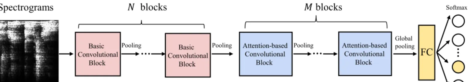
Based on frequency-distributed spectrogram, the proposed FreqCNN model combines CNNs with attention mechanism for feature learning. The overall architecture of the FreqCNN model is illustrated inFig. 4. Spectrograms are extracted from audio signals as the input for the subsequent CNN blocks. There are two types of convolutional blocks: basic convolutional blocks and attention-based convolutional blocks. These two types differ in whether there is an attention mechanism in the convolutional block. After several convolutional blocks, the output is connected to the fully connected layers. Finally, a fully connected layer with a softmax classifier outputs thefinal result.

Fig. 1.Examples of spectrograms for speech with different emotions: angry, sad and happy. Frequencies are shown increasing vertically and the horizontal axis represents time.

In the following text, we present details, accompany with examples, of basic convolutional blocks and attention-based convolutional blocks in the FreqCNN model.

4.1. Basic convolutional blocks

A spectrograms can be split into different frames within the time domain[14,15]and is called time-distributed spectrogram, as shown in

Fig. 5(a). Each split part includes the whole frequency domain at a certain time interval. In our work, the spectrogram is split into small segments along the frequency axis, as illustrated inFig. 5(b). Our idea is to pay attention to the energy distribution in different frequency in-tervals over the entire time window. At the same time, the whole spectrogram is also feed into the model to generate a global feature representation.

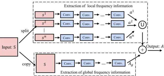
Fig. 6gives a general module of the basic convolutional block. In particular, for each basic block, we perform three steps:first, to obtain the frequency-distributed input, we split the whole frequency-time domain into several local regions along the frequency axis; second, we use multiple convolutional layers to learn different features. Based on the local information input, the model learns the local feature re-presentation as well as the whole frequency-time input; last, we com-bine the local and global feature representation to form the output of the block.

LetSdenote the input of the convolutional block. We split the input

S inton local parts (along the vertical axis) and the frequency-dis-tributed input set is denoted as {(s1,s2_{, ... ,s}n_{),S}, wheres}n_{is the data at}

thenth local frequency interval. Convolutions are performed separately on the set of frequency-distributed parts and the whole input. The ex-tracted features from different input can be described as follows: ⎧ ⎨ ⎩ = + ≤ ≤ = + a f w s b k n A g w S b ( ) (1 ) ( ) , k k k k g ₍₇₎

wherewk_{denotes the weight for thekth local frequency informations}k

andbk_{is the bias parameter. In addition,wdenotes the weight for the}

whole spectrogram S and bis the bias. Functions f( · ) and g( · ) are

activation functions in learning the local and global features, respec-tively. Note that we only giveEq. (7)to represent the operation of one convolutional layer for simplicity.

After concatenating all local features, we combine them with the global feature representation using element-wise addition as follows:

= + …

A Ag [ ;a a1 2; ;an], (8)

whereAdenotes thefinal output of the basic convolutional block.

Fig. 7(a) gives an example of the basic convolutional block. The input is split into two local frequency parts, so the frequency-dis-tributed input set is denoted as {(s1_,s2_{),S}. Global dataSis followed by}

two convolutional layers and the output of the convolution isAg.

Out-puts for frequency-distributed set s1 and s2 after one convolutional layer, i.e.,a1_anda2_{, are concatenated together. Finally, global feature}

Agplus the concatenation of local featuresa1,a2are used to compute

thefinal outputA.

4.2. Attention-based convolutional blocks

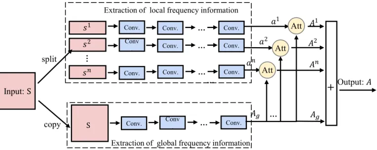
In a basic convolutional block, we simply add the global feature and the concatenation of all local features. In the attention-based convolu-tional block, utilizing CNNs with an attention mechanism, the model learns to reorganize the global feature representation.Fig. 8illustrates the structure in the attention-based convolutional block, where the attention method is used to guide the model to focus on more re-presentative parts. Using different local features, the model reorganizes them to form a new global feature representation. By aggregating all attention-based global features and the original global representation, we obtain thefinal output of the attention-based convolutional block. Attention methods are generally feature-based or spatial-based. As shown inFig. 3, a global feature representationAgmay be composed of

a set of local parts{ ,p₁ …,p_m}, wherem denotes the number of local parts. For different attention methods, the definition of the local parts differs.

Given frequency-distributed input {(s1_,s2_{, ... ,s}n_{),S}, there are a set}

of local features (a1,a2, ... ,an) and global featureAg. By taking certain

Input

:

Output

:

(a) The convolutional layer

Input

:

Output

:

(b) The pooling layer

Fig. 2.Convolution and pooling operations in a typical CNN architecture.

the number of feature maps:

…

(a) Spatial-based method

the shape of feature maps:

…

(b) Feature-based method

Fig. 3.Two kinds of attention methods for CNNs. Each feature map is organized as a rectangle in thisfigure.

local feature ak_{(1≤k≤n) into consideration, the attention method}

assigns weighth_i( )k to different local partspi(0≤i≤m), to obtain a

new global representationAk. As shown inEq. (9), the weighthi( )k for

local partpiis computed by two fully-connected layers:

= + + = …

hik g W f W p a( ( [ ;i k] b) b), i 1, ,m,

( )

2 1 1 2 (9)

wheref( · ) andg( · ) are activation functions. MatricesW1,W2are the

weight of thefirst and second layer, respectively, andb1andb2denote

the bias parameters of different layers. The weighted global feature representation can then be computed as follows:

= ⋯

Ak [p hk;p hk; ;p h ], m mk

1 1( ) 2 2( ) ( ) (10)

whereAkdenotes the attention-based global feature, which is based on corresponding local featureak_.

Finally, we combine all attention-based global features and the original global representation without attention. The output of atten-tion-based convolutional block is computed as follows:

∑

= + = A A A . k n k g 1 (11)

wherendenotes the number of parts in the frequency-distributed set.

Fig. 7(b) presents an example of attention-based convolutional block. The input is also split into two local parts. The global feature is

Agand local representation area1anda2. Further more, we applya1to

attention global feature Agand obtainA1, similarly available for A2.

Finally, addingAg, A1andA2are calculated as the output of

attention-based block.

5. Experiments

The proposed model is a general model for audio classification tasks, thus, we evaluated the FreqCNN model on three audio classifi -cation tasks: (a) accent classifi-cation; (b) speaker identifi-cation; and (c) speech emotion recognition.

For accent classification, the performance of FreqCNN was com-pared with the performance of the state-of-the-art method[2]and ex-isting CNN models, i.e., VGG[12]and ResNet[13]. We further explored the performance of the model using a different number of frequency-distributed set and two attention methods. In the speaker identification task, we compared our model with the traditional method (i.e., MFCCs)

[17]and typical CNN models. We also tested the FreqCNN model under different activation functions. In the speech emotion recognition ex-periment, we compared the performance of the proposed model with other related works[5,6,34,35]and presented a confusion matrix of the final recognition.

For all experiments, the extraction algorithm of the spectrograms was implemented using MIRtoolbox.1The sampling rate of all records was set to 16 kHz and the size of spectrograms in each experiment was different because of different database scales. The implementation of the FreqCNN is based on the MxNet framework.2We used stochastic gradient descent (SGD) with mini-batches. The learning rate started from 0.01, with a weight decay of1.0e − 8and a momentum of 0.9. All models were trained from scratch on Nvidia Tesla K40 GPUs.

Spectrograms

…

blocks

blocks

Pooling Pooling Global pooling

FC

Basic Convolutional Block Attention-based Convolutional Block Softmax

…

Basic Convolutional Block Attention-based Convolutional Block

…

Pooling

Fig. 4.The Architecture of the proposed FreqCNN model.

Fig. 5.Visual presentation of spectrograms. Two forms of spectrograms are illustrated: the time-distributed spectrogram and frequency-distributed spectrogram.

1_{http://www.mathworks.com/matlabcentral/fileexchange/}

24583mirtoolbox/.

2_{http://mxnet.io/MxNet is a scientific computing framework supporting}

5.1. Accent classification

Accent classification recognizes the difference in accents in one language or dialect. In this experiment, we examine the performance of the FreqCNN model on the UT-Podcast corpus[2].

Database and setting. The UT-Podcast corpus was designed to assist English accent research. It includes English accents from Australia (AU), the United States (US), and the United Kingdom (UK). InTable 1, we give the distribution of audio samples for each accent label. There are 1101 samples for training and 661 samples for testing. We randomly over-sampled some audio for training because of the class imbalance problem. The number of samples used for the experiment is given in

Table 1, denoted as Total2. In this experiment, spectrograms were

extracted with a size of 256 × 256 and the batch size was 48.

The best parameters of FreqCNN are listed inTable 2. There arefive convolutional blocks, including three basic blocks (BC) and two at-tention-based blocks (AC). Each input of the block is divided into two local parts. There are two convolutional layers for global features ex-traction and one layer for local features. All 3 × 3, 5 × 5, and 7 × 7 convolutions have corresponding zero-padding to retain the size of the receptive field after convolution. We adopted batch normalization layers right before each activation and convolutional layer.

Results and discussion. Hansen and Liu[2]achieved the state-of-art UAR of 74.5% on the UT-Podcast corpus using i-Vector. However, the FreqCNN model exhibits superior performance, achieving a UAR of up to 79.32%. The evaluation of recall score and unweighed average recall (UAR) are illustrated inTable 3. Moreover, several popular DNN architectures were tested in this experiment. We selected some typical CNN architectures with their default hyper-parameters, i.e., AlexNet

Output:

Conv.

split

copy

…

Conv.

Conv.

Conv.

+

Input:

Extraction of global frequency information

Conv.

…

Conv.

Conv.

…

Conv.

Conv.

…

Conv.

Conv.

…

Conv.

Extraction of local frequency information

Fig. 6.General module of a basic convolutional block. In this block,“∪”indicates concatenation and“+”indicates element-wise addition.

local:

global:

Conv.

Conv.

Conv.

Conv.

Addition

Input:

local:

Output:

Concatenate

(a) Basic convolutional block

local:

global:

Conv.

Conv.

Conv.

Conv.

Addition

Input:

Attention

Attention

local:

Output:

(b) Attention-based block

[36], VGG-11[12]and ResNet-18[13]. AlexNet is a typical CNN with five convolutional layers and two fully-connected layers. VGG and ResNet have deeper architecture with more convolutional layers. Because of the small dataset, we further designed two small DNN models: a three-layer FNN and afive-layer CNN. As shown inTable 3, FreqCNN achieves the best performance among these models, followed by i-vector method and AlexNet model. Especially, small DNNs (AlexNet and 5-layer CNN) can achieve better results than lager models (VGG-11 and ResNet-18). AlexNet is much better than other methods in the recognition of UK, which is just lower than our proposed method. 5-layer CNN is much better than other methods in the recognition of US, which is just lower than i-vector method. Compared with these methods, our model achieves the best performance in two out of three categories (AU and UK) and its average score is the best. These results demonstrate that the combination of global and local features and the use of attention with CNNs indeed improve the recognition performance.

Furthermore, we evaluated the performance of the model using different numbers of frequency-distributed segments (0, 2, 4, 8) under two kinds of form: local frequency only and the combination of global

Output:

Conv.

split

copy

…

Conv

.

Conv.

Conv.

Input:

Extraction of global frequency information

Conv

.

…

Conv.

Conv.

…

Conv.

Conv.

…

Conv.

Conv.

…

Conv.

Extraction of local frequency information

Att

Att

…

…

Att

+

Fig. 8.The structure of the attention-based convolutional block.

Table 1

The number of training and testing records per accent.

#Samples Accent Total

AU US UK UK2 Original Over-sampled

Training 449 406 246 492 1101 1347

Testing 332 240 89 89 661 661

Table 2

Best parameters of the FreqCNN model in accent classification on the UT-Podcast.

Name Local convolution Global convolution Pooling

Basic block 1 64, 5 × 5/1, sigmoid 64, 5 × 5/1, tanh

Conv. and pool 64, 7 × 7/1 max, 2 × 2/2

Basic block 2 64, 5 × 5/1, sigmoid 64, 5 × 5/1, tanh

Conv and pool 96, 7 × 7/1 max, 2 × 2/2

Basic block 3 96, 5 × 5/1, sigmoid 96, 5 × 5/1, tanh

Conv. and pool 128, 7 × 7/1 max, 2 × 2/2, dropout 0.2

Attention-based block 4 128, 5 × 5/1, sigmoid 128, 3 × 3/1, tanh

fc: 512, tanh; 256, tanh; 1, sigmoid

Conv. and pool 256, 5 × 5/1 max, 2 × 2/2, dropout 0.2

Attention-based block 5 256, 3 × 3/1, sigmoid 256, 3 × 3/1, tanh

fc: 256, tanh; 1, sigmoid

Conv. and pool 256, 512, 5 × 5/2, tanh avg (global), dropout 0.5

fc 512, relu, dropout 0.5

Softmax 3-way softmax

Table 3

Recall and UAR (%) of different models on the UT-Podcast.

Recall Methods

i-Vector FreqCNN FNN CNN AlexNet VGG-11 ResNet-18 AU 78.00 88.55 70.78 64.76 58.43 55.72 69.28 UK 61.80 71.91 50.56 41.57 64.04 48.31 38.20 US 83.80 77.50 62.92 82.08 74.17 59.17 77.50 UAR 74.50 79.32 61.42 62.81 64.90 54.40 61.66

Table 4

Comparison of local frequency segments and global-local frequency with dif-ferent numbers of local partial frequency.“0”partial frequency segment means there is only global spectrogram used.

Evaluation Number of partial frequency

0 2 4 8

Local frequency only UAR − 70.53 75.86 70.27

ACC − 76.85 79.27 73.22

Global and local frequency UAR 72.45 75.41 77.68 76.38

and local frequency. Experimental results are listed inTable 4. Com-pared with only local frequency method or only global information method, the combination of global and local frequency indeed improves the recognition performance. The experimental results show that the best accuracy is up to 80.18%, using the global frequency and 4 partial frequency information together. With global frequency only method, the model can obtain accuracy of 74.89% and recall rate of 72.45%. With local frequency-distributed segments only method, the model can get better accuracy of 79.27% when the number of local parts is 4. As the number of local frequency segments continues to increase, the number of parameters in the model also increases. The performance does not improve.

We also compared the performance of time-distributed form and frequency-distributed form of spectrograms, under different attention-based blocks and attention techniques. There are all two local parts in frequencies or time in each experiment. The results are illustrated in

Table 5. These experiments demonstrate that attention technique in-deed improves the recognition performance in accuracy and UAR,

compared with no attention in the model, for both splitting spectro-grams in frequencies or time. Moreover, the overall recognition for frequency-distributed spectrograms is higher than time-distributed spectrograms. In the frequency-distributed form, feature-based atten-tion gives us the best result in the last two convoluatten-tional blocks, achieving an accuracy of 82.30%, and spatial-based attention achieves better performance when it is only used in the last convolutional block. In the time-distributed form, spatial-based attention improves accuracy a lot but UAR slightly. Feature-based attention obtains the best result in the last convolutional block, achieving the UAR of 75.88%.

5.2. Speaker identification

Speaker identification determines who is the speaking person. A well-trained text-independent identification model can recognize a speaker from any text, even without training. In this experiment, we tested the FreqCNN model of a text-independent task on the CHAINS corpus[17].

Database and setting. The CHAINS speech corpus is designed to characterize different speakers. The corpus contains 36 speakers, and each speaker provides speech of all text in six different speaking styles, such as solo, synchronous, and retelling. In this experiment, only solo reading was used. A code is provided for six independent text paragraphs: { (01), (02), (03), (04), 01f f f f s −s09, 10s −s33}. For brevity,s01−s09is calleds(01) ands10−s33is calleds(02). For a text-independent speaker identification task, four out of six paragraphs were used for training and the two remaining ones were used for testing. Finally, we adopted three-fold cross-validation for the average accuracy. Details for the training and testing sets are listed inTable 6. Spectrograms were extracted as a size of 224 × 224 and the number of batch sizes was 128.

The best parameters of the FreqCNN model for this task are given in

Table 7. Similarly, there were two convolutional layers for global fea-ture extraction and one layer for local feafea-tures. We also adopted batch normalization layers right before the convolutional layers and zero-padding in the convolution.

Results and discussion. The results of the FreqCNN model, i-vector and typical CNN models with three-fold cross-validation are given in

Table 8. Compared with the traditional method [17] using MFCCs with vector quantization and gaussian mixture model, which obtains an accuracy of 91.00%, our model improves accuracy around +7% and obtains a UAR of 98.05% on average. We also tested i-vector and Table 5

Comparison of two ways of attention methods in CNNs and different numbers of attention-based blocks.“1 A”means that only the last convolutional block uses attention and“2 AC”means that the last two convolutional blocks use atten-tion.“All BC”indicates that there is no attention in the FreqCNN model.

Attention Feature-based methods

Spatial-based methods

ACC UAR ACC UAR

Frequency- distributed All BC ACC: 76.10 UAR: 75.41

1 AC 78.37 75.77 77.91 76.33

2 AC 82.30 79.32 74.28 74.74

3 AC 76.55 73.67 77.46 72.59

Time-distributed All BC ACC: 74.43 UAR: 73.27

1 AC 74.74 75.88 77.46 73.88

2 AC 73.37 74.46 77.31 74.08

3 AC 70.65 66.40 75.34 73.81

Table 6

Details of three-fold data set of the CHAINS corpus.

No. Training #Samples Validation #Samples

#1 f(03), f(04), s(01), s(02) 2484 f(01), f(02) 1530 #2 f(01), f(02), s(01), s(02) 2718 f(03), f(04) 1296 #3 f(01), f(02), f(03), f(04) 2826 s(01), s(02) 1188

Table 7

Best parameters of the FreqCNN model in speaker identification on the CHAINS.

Name Local convolution Global convolution Pooling

Basic block 1 32, 5 × 5/1, sigmoid 32, 5 × 5/1, sigmoid

Conv. and pool 32, 7 × 7/1 max, 2 × 2/2

Basic block 2 32, 5 × 5/1, sigmoid 32, 5 × 5/1, sigmoid

Conv and pool 32, 7 × 7/1 max, 2 × 2/2

Basic block 3 64, 5 × 5/1, sigmoid 64, 5 × 5/1, sigmoid

Conv. and pool 64, 7 × 7/1 max, 2 × 2/2, dropout 0.2

Attention-based block 4 96, 5 × 5/1, sigmoid 96, 3 × 3/1, sigmoid

fc: 256, tanh; 128, tanh; 1, sigmoid

Conv. and pool 256, 5 × 5/1 max, 2 × 2/2, dropout 0.2

Attention-based block 5 128, 3 × 3/1, sigmoid 128, 3 × 3/1, sigmoid fc: 128, tanh; 1, sigmoid

Conv. and pool 256, 5 × 5/2, tanh avg (global), dropout 0.5

fc 128, relu, dropout 0.5

several CNN models with their default hyper-parameters on the CHAINS. The evaluation of Equal Error Rate (EER) and threshold in i-vector method is given by Kaldi speaker recognition system.3_{EER is} calculated using the method proposed in the paper [37], which is different from Error Rate (ERR). The experimental results show that our proposed model obtained the highest accuracy and UAR among all methods. On the whole, i-vector, VGG-11 and ResNet-18 achieve better result than other CNN models (ResNet-34 and ResNet-50). I-vector and VGG-11 have better recognition performance in the data set #3. More importantly, the performance of the FreqCNN model is vastly better than other methods in all three-fold experiments.

InTable 9, we also compared FreqCNN models using different ac-tivation functions in the convolutional layers. The lowest accuracy is 90.76% when the activation functions of convolutional layers in global and local feature learning are relu and tanh, respectively. The combi-nation of sigmoid and tanh always yield good performance. From these results, it can be concluded the FreqCNN model can get the best result when the activation function of convolutional layers in both local and global feature extraction is a sigmoid function.

5.3. Speech emotion recognition

The aim of speech emotion recognition is to distinguish emotional states from speech signals such as anger, happiness, and sadness. A speaker-independent task means that speakers in the training set are mismatched with those in the testing set. In this experiment, a speaker-independent task was conducted on the eNTERFACE speech corpus[6].

Database and setting. The eNTERFACE database is an audio-visual English emotional corpus that includes 42 speakers. Only speech signals extracted from the video are used in this experiment. Each speaker has 30 records for six types of emotions, namelyhappiness, anger, disgust, fear, sadness, and surprise. The distribution of data samples for each emotion label in the dataset is balanced. In this experiment, we used ten-fold cross-validation methods; i.e., we leave four orfive speaker records for testing in turns. Spectrograms were extracted as a size of 224 × 224 in this experiment and the batch size was set to 48.

The best parameters of the FreqCNN model for speech emotion re-cognition task are given inTable 10. Similarly, there are three con-volutional blocks and two attention-based concon-volutional blocks. In each Table 8

ACC and UAR (%) of the proposed model and typical DNNs on the CHAINS. I-Vector* denotes the metrics of (1−EER) and threshold in the bracket.

Methods data set #1 data set #2 data set #3 Average

ACC UAR ACC UAR ACC UAR ACC UAR

FreqCNN 99.08 99.08 99.85 99.86 95.20 95.21 98.04 98.05 VGG-11 70.52 70.52 78.16 77.85 76.94 76.95 75.21 75.11 ResNet-18 86.47 86.35 89.58 89.49 49.07 49.11 75.04 74.99 ResNet-34 71.96 72.04 77.55 77.25 48.65 48.70 66.05 66.00 ResNet-50 73.14 73.00 76.77 76.29 50.93 50.96 66.95 66.75 i-Vector* 72.93 (−2.46241) 83.17 (−3.04434) 58.43 (30.2318) Table 9

ACC and UAR (%) of different activation functions.g( · ) denotes the activation of convolutional layers for the global feature learning andf( · ) denotes the activation in the local domains.

Activation function data set #1 data set #2 data set #3 Average

g( · ) f( · ) ACC UAR ACC UAR ACC UAR ACC UAR

Sigmoid sigmoid 99.08 99.08 99.85 99.86 95.20 95.21 98.04 98.05 Sigmoid tanh 98.17 98.21 99.61 99.65 93.94 93.94 97.24 97.27 Tanh sigmoid 98.43 98.44 99.15 99.17 95.45 95.47 97.68 97.69 Tanh tanh 99.02 99.09 99.31 99.34 93.52 93.53 97.28 97.32 Tanh relu 99.35 99.42 99.23 99.28 90.74 90.79 96.44 96.50 Relu tanh 95.88 95.99 99.54 99.52 76.85 76.92 90.76 90.81 Relu relu 96.08 96.17 98.69 98.68 85.94 86.01 93.57 93.62 Table 10

Best parameters of the FreqCNN model in speech emotion recognition on the eNTERFACE.

Name Local convolution Global convolution Pooling

Basic block 1 64, 5 × 5/1, sigmoid 64, 5 × 5/1, tanh

Conv. and pool 96, 7 × 7/1 max, 2 × 2/2

Basic block 2 96, 5 × 5/1, sigmoid 96, 5 × 5/1, tanh

Conv and pool 128, 7 × 7/1 max, 2 × 2/2

Basic block 3 128, 5 × 5/1, sigmoid 128, 5 × 5/1, tanh

Conv. and pool 128, 7 × 7/1 max, 2 × 2/2, dropout 0.2

Attention-based block 4 256, 5 × 5/1, sigmoid 256, 3 × 3/1, tanh

fc: 256, tanh; 128, tanh; 1, sigmoid

Conv. and pool 256, 5 × 5/1 max, 2 × 2/2, dropout 0.2

Attention-based block 5 256, 5 × 5/1, sigmoid 256, 3 × 3/1, tanh

fc: 256, tanh; 1, sigmoid

Conv. and pool 512, 512, 5 × 5/2, tanh avg (global), dropout 0.5

fc 512, relu, dropout 0.5

Softmax 6-way softmax

block, there are two convolutional layers for global feature extraction and one layer for local features. We also adoptedsigmoidandtanh ac-tivation functions.

Results and discussion. The accuracy of our model and other prominent methods are listed in Table 11. Compared with previous approaches

[5,6,34,35], our proposed model obtains more robust performance and achieves an accuracy 83.62%. To consider the characteristics of spectrograms, we replaced the simple DNNs by a deep convolutional model with an attention mechanism. The latest method[35]also obtain good results using three-dimensional CNNs (3D-CNNs) and deep belief networks. Though other studies used well-designed feature sets or models, to the best of our knowledge, we manage to outperform the state-of-the-art accuracy in the speaker-independent case.

Further,Table 12shows the confusion matrix of the best results in the speaker independent task. The highest accuracy is obtained for surprise (88.57%), followed by angry (85.71%). The lowest accuracy yielded for sadness (78.57%). Disgust also has a low accuracy (79.52%). This may be because the recognition of less active and unpleasant emotions is more difficult. The average recognition rate over all emo-tions is 83.65%.

5.4. Discussion

Experiments have shown that for different audio classification tasks, the FreqCNN model brought in different performance improving than traditional methods or DNNs. For different tasks, the architecture of the FreqCNN model is instantiated, by making some changes in the number of convolutional blocks,filters, activation functions, attention and etc. It can be concluded the proposed model has the generalization over different audio classification tasks with prominent performance. 6. Conclusions

This paper proposed a generic framework for different audio clas-sification tasks. Based on the characteristics of spectrograms, the FreqCNN model uses a novel frequency-distributed form of spectro-grams and combines them with CNNs and attention. These convolu-tional blocks consider both local frequency areas and the global fre-quency-time domain to enable them to learn more distinctive audio-related features. Furthermore, we applied the principle of attention to assist the learning of the frequency-distributed feature set, which

improves recognition performance. In the experiment, we used the FreqCNN model to perform multiple audio classification tasks. To the best of our knowledge, we outperform the state-of-art results on these speech databases.

Acknowledgment

This work was supported by the National Science Foundation of China (Grant No. 61432012, 61502322) and Sichuan Science and Technology Program (Grant No. 2018JY0018, 2017JY0258).

References

[1] M. Akagi, X. Han, R. Elbarougy, Y. Hamada, Toward affective speech-to-speech translation: Strategy for emotional speech recognition and synthesis in multiple languages, Proceedings of the Signal and Information Processing Association Summit and Conference, (2015), pp. 1–10.

[2] J.H.L. Hansen, G. Liu, Unsupervised accent classification for deep data fusion of accent and language information, Speech Commun. 78 (2016) 19–33.

[3] L. He, M. Lech, N.C. Maddage, N.B. Allen, Time-frequency feature extraction from spectrograms and wavelet packets with application to automatic stress and emotion classification in speech, Proceedings of the International Conference on Information, Communications and Signal Processing, (2009), pp. 1–5. [4] Z. Qawaqneh, A.A. Mallouh, B.D. Barkana, Deep neural network framework and

transformed MFCCs for Speaker’s age and gender classification, Knowl. Based Syst. 115 (C) (2017) 5–14.

[5] C.S. Ooi, S.K. Phooi, L.-M. Ang, L.W. Chew, A new approach of audio emotion recognition, Expert Syst. Appl. 41 (13) (2014) 5858–5869.

[6] S. Poria, E. Cambria, A. Hussain, G.-B. Huang, Towards an intelligent framework for multimodal affective data analysis, Neural Netw. 63 (2015) 104–116.

[7] T.F. Li, S.-C. Chang, Speech recognition of mandarin syllables using both linear predict coding cepstra and mel frequency cepstra, Proceedings of the Conference on Computational Linguistics and Speech Processing, (2007), pp. 379–390. [8] Z. Yi, Foundations of implementing the competitive layer model by Lotka-volterra

recurrent neural networks, IEEE Trans. Neural Netw. 21 (3) (2010) 494. [9] F. Li, L. Tran, K.-H. Thung, S. Ji, D. Shen, J. Li, A robust deep model for improved

classification of AD/MCI patients, IEEE J. Biomed. Health Inf. 19 (5) (2015) 1610–1616.

[10] Y. Zhu, S. Lucey, Convolutional sparse coding for trajectory reconstruction, IEEE Trans. Pattern Anal. Mach. Intell. 37 (3) (2015) 529.

[11] Y. LeCun, Y. Bengio, G. Hinton, Deep learning, Nature 521 (7553) (2015) 436–444. [12] K. Simonyan, A. Zisserman, Very deep convolutional networks for large-scale image

recognition, Comput. Sci. (2014).

[13] K. He, X. Zhang, S. Ren, J. Sun, Deep residual learning for image recognition, Proceedings of the IEEE Conference on Computer Vision and Pattern Recognition, (2016), pp. 770–778.

[14] M. Espi, M. Fujimoto, K. Kinoshita, T. Nakatani, Exploiting spectro-temporal lo-cality in deep learning based acoustic event detection, Eurasip. J. Audio Speech Music Process. 2015 (1) (2015).

[15] W. Lim, D. Jang, T. Lee, Speech emotion recognition using convolutional and re-current neural networks, Proceedings of the Signal and Information Processing Association Summit and Conference, (2016), pp. 1–4.

[16] Y. Leng, C. Sun, X. Xu, Q. Yuan, S. Xing, H. Wan, J. Wang, D. Li, Employing un-labeled data to improve the classification performance of SVM, and its application in audio event classification, Knowl. Based Syst. 98 (C) (2016) 117–129. [17] N.M. AboElenein, K.M. Amin, M. Ibrahim, M.M. Hadhoud, Improved

text-in-dependent speaker identification system for real time applications, Proceedings of the Fourth International Japan-Egypt Conference on Electronics, Communications and Computers, (2016), pp. 58–62.

[18] H. Bourlard, S. Dupont, A new ASR approach based on independent processing and recombination of partial frequency bands, Proceedings of the International Conference on Spoken Language Processing, (1996).

[19] H. Bourlard, S. Dupont, Subband-based speech recognition, Proceedings of the IEEE International Conference on Acoustics, Speech and Signal Processing, (1997), pp. 1251–1254.

[20] X.U. Jing-Bo, Y.U. Hong-Tao, C.S. Ran, Speech enhancement using sub-band spec-tral analysis, J. Appl. Sci. 24 (3) (2006) 232–235.

[21] J. Du, Y. Xu, Hierarchical deep neural network for multivariate regression, Pattern Recognit. 63 (2017) 149–157.

[22] J. Du, Irrelevant variability normalization via hierarchical deep neural networks for online handwritten chinese character recognition, Proceedings of the International Conference on Frontiers in Handwriting Recognition, (2014), pp. 303–308. [23] R.A. Rensink, The dynamic representation of scenes, Vis. cogn. 7 (1–3) (2000)

17–42.

[24] K. Xu, J. Ba, R. Kiros, K. Cho, A. Courville, R. Salakhudinov, R. Zemel, Y. Bengio, Show, attend and tell: neural image caption generation with visual attention, Proceedings of the International Conference on Machine Learning, (2015), pp. 2048–2057.

[25] V. Mnih, N. Heess, A. Graves, et al., Recurrent models of visual attention, Proceedings of the Advances in Neural Information Processing Systems, (2014), pp. 2204–2212.

[26] M.F. Stollenga, J. Masci, F. Gomez, J. Schmidhuber, Deep networks with internal Table 12

Confusion matrix of the best result of the FreqCNN model on the eNTERFACE.

Actual Classification Predicted Classification

Angry Disgust Sadness Surprise Fear Happiness

Angry 180 8 3 12 5 2 Disgust 8 167 5 13 10 7 Sadness 6 4 165 14 15 6 Surprise 3 2 3 186 6 10 Fear 4 5 6 12 178 5 Happiness 2 5 4 11 10 178 Table 11

Results of the FreqCNN model and other state-of-the-art proposals in the audio modality on the eNTERFACE.

Input Methods ACC (%)

MFCC, BDPCA, LDA features[5] RBF 75.89

Spectrograms[34] DNNs 60.53

Long, short time-based features[6] SVM 78.57

Mel-spectrograms[35] 3D-CNN, DBN 78.08

selective attention through feedback connections, Proceedings of the Advances in Neural Information Processing Systems, (2014), pp. 3545–3553.

[27] A. Mencattini, E. Martinelli, G. Costantini, M. Todisco, B. Basile, M. Bozzali, C.D. Natale, Speech emotion recognition using amplitude modulation parameters and a combined feature selection procedure, Knowl. Based Syst. 63 (C) (2014) 68–81.

[28] O. Ghahabi, J. Hernando, Deep belief networks for i-vector based speaker re-cognition, Proceedings of the IEEE International Conference on Acoustics, Speech and Signal Processing, (2014), pp. 1700–1704.

[29] A. Kanagasundaram, R. Vogt, D. Dean, S. Sridharan, M. Mason, I-vector based speaker recognition on short utterances, Proceedings of the INTERSPEECH, (2011). [30] W.Q. Zheng, J.S. Yu, Y.X. Zou, An experimental study of speech emotion recogni-tion based on deep convolurecogni-tional neural networks, Proceedings of the Internarecogni-tional Conference on Affective Computing and Intelligent Interaction, (2015), pp. 827–831.

[31] H. Lee, P. Pham, Y. Largman, A.Y. Ng, Unsupervised feature learning for audio classification using convolutional deep belief networks, Proceedings of the Advances in Neural Information Processing Systems, (2009), pp. 1096–1104.

[32] Z. Fu, G. Lu, K.M. Ting, D. Zhang, Optimizing cepstral features for audio classifi -cation. Proceedings of the International Joint Conference on Artificial Intelligence, (2013), pp. 1330–1336.

[33] S. Scardapane, D. Comminiello, M. Scarpiniti, R. Parisi, A. Uncini, Benchmarking functional link expansions for audio classification tasks, Proceedings of the Advances in Neural Networks, (2016), pp. 133–141.

[34] H.M. Fayek, M. Lech, L. Cavedon, Towards real-time speech emotion recognition using deep neural networks, Proceedings of the International Conference on Signal Processing and Communication Systems, (2015), pp. 1–5.

[35] S. Zhang, S. Zhang, T. Huang, W. Gao, Q. Tian, Learning affective features with a hybrid deep model for audio-visual emotion recognition, IEEE Trans. Circuits Syst. Video Technol. PP (99) (2017).

[36] A. Krizhevsky, I. Sutskever, G.E. Hinton, Imagenet classification with deep con-volutional neural networks, Proceedings of the International Conference on Neural Information Processing Systems, (2012), pp. 1097–1105.

[37] D.A. Reynolds, R.C. Rose, Robust text-independent speaker identification using gaussian mixture speaker models, IEEE Trans. Speech Audio Process. 3 (1) (1995) 72–83.