Toward Waste-Free Cloud Computing

Toward Waste-Free Cloud Computing

Tung Nguyen and Weisong Shi

Department of Computer Science

Wayne State University

{

nttung,weisong

}

@wayne.edu

Abstract

Many previous efforts focus on improving the utlization of data centers. We argue that even highly utilized sys-tems can still waste the resource because of failures and maintenance. Therefore, in this position paper, we call on a new direction of research on waste-free computing. We start with a workable definition of efficiency, then in-troduce a new efficiency metric calledusage efficiency, show how to compute it and propose some possible ap-proaches to improve this type of efficiency. We also cal-culate the metric through the simulation on real failure traces and diverse workflow applications. While the ef-ficiency computed from the traditional method is 100%, it is less than 44% with our new metric which suggests that the current metrics are inadequate to capture the ef-ficiency of a system.

1

Introduction

We have witnessed the fast growing of large-scale data centers because of the promise of cloud computing, run-ning either publicly or privately. In this position paper, we argue that computing resources in those facilities are not being used efficiently. They are eitherunder-utilized

ordoing meaningless work. Next we will use four

exam-ples to support this argument.

Observation 1: Schroeder and Gibson [22] envision that, by 2013, the utilization of a top500 computer (top500.org) may drop to 0% based on their assumption about the growth in number of cores per socket and the checkpoint overhead. This is because the only job that a future system would be busy with is checkpointing due to the fact that the number of failures in future computers would increase proportionally to the number of cores.

Observation 2: In a typical industrial data center, the average utilization is only 20 to 30 percent [4, 6] (due to the QoS guarantee for example). However, such low utilized or idle servers still draw 60% of the peak

power [4, 14, 11]. The average CPU utilization of 5000 Google servers in 6 months is in the 10-50% range which is in the most energy inefficient region [3].

Observation 3: In systems that offer infrastructure as a service (IaaS), the virtualization may lead to low utiliza-tion too. Basically, virtualizautiliza-tion techniques allow us to “cut” a physical machine into isolated virtual machines. The inefficiency comes not only from the overhead of the splitting process itself but also from the mismatching between virtual and real resources especially in heteroge-neous systems. For example, an old machine with only 1.5GHz processor can only offer one EC2-like standard instance(1-1.2GHz) and the rest is wasted.

Observation 4: Together with the rapid penetration of multicore architectures, the utilization of these cores be-comes a big issue. It’s quite common to see that one core is very busy while the other ones are pretty idle. For ex-ample, when executing the serial part of a program, only one core is needed and others are idle [12]. Furthermore, the issues of maintaining consistency, synchronization, communication, scheduling between many cores might introduce considerable overhead too.

Based on these observations, we categorize the wasted resources into two types:wasted under-utilized resource

and wasted utilized resource. The first type, wasted

under-utilized resource, is the difference between the

available (physical) resources and the consumed re-sources. It is caused by the low utilization as in the “Ob-servations 2, 3 and 4”. It is used to answer the question:

how many percentages of the available resources are

uti-lized? The second type,wasted utilized resource, is the

difference between the consumed resources and the

use-ful resources(spent on users’ jobs). It is often caused by

the administrative or maintenance tasks as in the “Obser-vation 1 and 4”. It is used to answer the question:Among utilized resources, how many percentages are spent on doing useful work?

In addition, the need for resources such as energy is

is approaching. Most data, applications and computa-tion are moving into Cloud. This trend will obviously increase the need of more powerful data centers which are energy hungry. Silicon Valley Leadership Group has also forecasted this increasing trend in the data center en-ergy use based on the Environmental Protection Agency (EPA) reported earlier in 2007 [2, 10].

As a result, using resourceefficientlyorminimizing the

wasteis becoming a very important issue. Minimizing

the wasted under-utilized resources, i.e. maximizing the utilization of resources, has been a hot topic in both aca-demic and industrials, such as data center designs and cloud vendors, in order to improve their sustainability. In this paper, we argue that improving the resource uti-lization is useful, however, is not enough. We also need to reduce the resource wasted for other purposes such as failures and maintenance (wasted utilized resources). For example, if during its execution, one critical task fails re-sulting the start-over of the whole job, the resources have been used before the failure are wasted. We envision that those types of resource waste, which are the root of the lower efficiency of computing, should be eliminated sig-nificantly. Therefore we introducewaste-free comput-ingwhich considers the efficiency from different angles.

2

Efficiency Computation

Essentially, efficiency is a multi-objective problem. Un-like the traditional systems dealing with single-objective optimization problems such as minimizing the execu-tion time, minimizing power consumpexecu-tion or maximiz-ing throughput, etc, efficient systems try to “do more with less”. It is obvious that there is a trade-off between objectives. The trade-off between benefits and cost is en-capsulated in one metric called efficiency. In this section, we will go over some widely used formulas to calculate the efficiency before deriving our own formula.

Generally, efficiency is defined as follows

Ef f iciency= Return

Cost (1)

TheReturncan be profit, the number of work done, im-provement of performance (execution time), throughput, bandwidth, availability, queries per second etc. TheCost is what we spend to obtain theReturnsuch as money, energy consumption, CPU time, storage space, etc.

Depending on specific Return and Cost, there are different types of efficiency. Let’s consider some exam-ples:

Example 1: in term of CPU time, the CPU efficiency is defined as the CPU time spent on doing useful work, di-vided by the total CPU time. Assume T is the processing time for each process before context switch could occur

and S is the overhead for each content switch. For round robin scheduling with quantum Q seconds:

CPU Efficiency= T T+S ifQ > T = T T+S×T Q ifS < Q < T (2)

Example 2: in term of energy, there are many levels of efficiency ranging from chip to data center. At proces-sor level, CPU efficiency is defined as the performance (MIPS) per joule or watt [20]. At storage level, stor-age efficiency is define as number of queries per second (QPS) per joule or watt [23].

At datacenter level, recent work [8, 9] has defined two widely used metrics (Power Usage Effectiveness (PUE) and Data Center Infrastructure Efficiency(DCiE)) to measure the data center infrastructure efficiency and compare the energy efficiency between data centers.

P U E= Total Facility Power

IT Equipment Power (3)

DCiE= IT Equipment Power

Total Facility Power ×100% (4) Arguing that PUE and DCiE “do not allow for mon-itoring the effective use of the power supplied – just the differences between power supplied and power con-sumed,” Gartner [7, 18] proposed a new metric called Power to Performance Effectiveness (PPE).

P P E = Useful Work

Total Facility Power (5)

Moreover, there is work that considers the combina-tion of efficiency at different levels. For example, in [3], Barroso and H¨olzle factorized the Green Grid’s Datacen-ter Performance Efficiency (DCPE) into 3 components to capture different types of energy efficiency such as facil-ity, server energy conversion, and electronic components (from large scale to small scale). They defined energy efficiency metric as (detail computation can be found in [9, 3, 8])

Energy Efficiency= Computation

Total Energy (6) = ₁ P U E × ₁ SP U E × _Computation

Total Energy to Electronic Comp.

The inefficiency is caused by the waste. Where does waste come from? In the first example, the waste is in CPU time. It comes from the context switch time and the scheduling algorithm. In the second example, the

waste is in energy. It comes from unsuitable, inefficient design, architecture, cooling, power conversion and dis-pensation, etc.

Apart from the previous types of efficiency, we intro-duce another type of efficiency calledusage efficiency. With this type, failure is the cause of inefficiency and re-source waste. For example, if users submit a job to the system, and it is assigned to unreliable nodes. If some of the nodes fail while executing their job (which is very likely with unreliable nodes), all resources consumed or cost spent on execution before failure are useless. This not only reduces the performance (increase the total exe-cution time) but also increases the total cost. Even worse, this can also affect the schedule of other jobs. Therefore, we introduce a new efficiency metric as the following.

Usage efficiency= Required Resource

Actual Resource Used (7) The objective is to minimize the number of job re-execution or, more precisely, reduce the probability to execute the job again.

3

Usage Efficiency Computation

In this section, we are going to compute the proposed usage efficiency. First we need to identify clearly what areRequired ResourceandActual Resource Used.

In our case, theRequired Resource is the total execution time of a job without failure and theActual Resource Usedis the actual execution time. The ex-ecution time is considered as a resource. The more time the job is executed, the more resource it consumes. In the perfect system, i.e. there is no failure, this type of efficiency has value of 1. The general equation (7) is rewritten as

Usage Efficiency= Total exec time w/o failure

Real total exec time (8) In the problem, ajobis composed ofk tasks. A job is executed onNprocessing instances (PI) which are either virtual or physical machines.

LetPi,(i = 1, N)be the probability that theithPI fails during the job execution time.

Each task has execution timetj(j= 1, k)

For simplicity, we assume thatN > k and each PI executes one thread. Therefore, if the PI fails, so does the task running on it. Also, we assume that the failure is of the type fail stop only.

For a job, if one task of a job fails, do we need to re-execute the whole job from the beginning, part of the job or just that task only? Can we reuse the results of the successful, completed tasks? This essentially depends on the dependencies among tasks. With the extremely

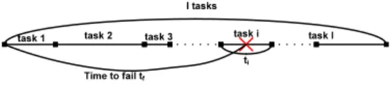
l tasks

t_i Time to fail t_f

task 1 task 2 task 3 task i task l

Figure 1: The real execution time of a job.

scale map-reduce like jobs, if one task fails, the system only needs to re-execute it. Unfortunately, not all appli-cations fall into such type. Many of them follow work-flow model and there are tasks that are correlated. In such model, we may need to replicate the execution of a task to mask the failure or store the intermediate data to avoid re-execution of the job from the beginning.

Assuming that we know the “critical execution path” of the job which the tasks on it decide the total execution time of the job (Figure 1). If any of them is delayed, so does the job. We consider two cases if any of such tasks fail: (1) the execution starts over from the beginning; (2) the execution just restarts the failing tasks. We don’t con-sider replicated execution here. Letlbe the length of the path(1 ≤l ≤ k). It’s also the number of tasks on that path.

3.1

Macro-rescheduling:

Re-execute the

whole job

The probability that all l critical nodes/tasks don’t fail during their execution isΠl

i=1(1−Pi).

Let Y be a random variable denotes the number of times that the job is re-executed. Iftask j is re-executed

on the same node after failure, and thefailure

probabil-ityPi of theithPI doesn’t changeamong executions,

Y follows Geometric distribution, and therefore has the expectation as the following.

E[Y] = 1 Πl

i=1(1−Pi)

Without failure, the total execution time of the job is the sum of all tasks on the critical path which isT = Σl

i=1ti.

With failure, in this case, the job is start-over from the beginning as shown in Figure 1. The probability that at least one critical task fails equals to the probability that the job is re-executed

P_{at least 1 fail}=P_re-executed= 1−Πl_i=1(1−Pi) It is noteworthy that although the time to fail is uni-formly distributed withintj for individual critical task j, it is different across tasks.

⇒the expected time to fail for each execution before the first success of the job is

Pl j=1tj

Let T be the real execution time of the job, andtfnbe the time to fail at thenthexecution of the job.

T =P_{at least 1 fail}× Y X n=1 tfn+ Πli=1(1−Pi)× l X j=1 tj

⇒the expected execution time of the job is

E[T] =P_{at least 1 fail}× E[Y]× Pl j=1tj 2 ! +Πl_i=1(1−Pi)× l X j=1 tj

3.2

Micro-rescheduling:

Re-execute the

failing tasks

In this case, the real execution time of the job is simply the sum of that of its individual tasks on the critical path. LetXibe a random variable denotes the number of times that taskithis re-executed.

T = l X i,j=1 Tij = l X i,j=1 pi× Xi X n=1 tfn+ (1−pi)×tj ! and we have E[T] = l X i,j=1 pi× E[Xi]× tj 2 + (1−pi)×tj

The usage efficiency for both rescheduling schemes is

Usage Efficiency=

l

X

j=1

tj/E[T]

For each job,tjare fixed, butpivary among machines, and their values even change over the time. Thesepican be obtained by failure prediction algorithms like [21, 16]. It is noteworthy that we made two very strong assump-tions about the re-execution mechanism and the failure probability. In reality, when a task fails, the scheduler can assign another PI, which has a different failure prob-ability, to take care of it. Also, even the failure probabil-ity of the same PI may change over the time. Relaxing these assumptions certainly complicates the above com-putation.

4

Usage Efficiency with Real Traces

After showing the computation of the usage efficiency in theory, in this section, we will use the real failure traces and varied workflows to derive the usage effi-ciency through simulation.

The failure in the simulation includes 10 two-month traces extracted from the real failure trace in [1]. It’s done by randomly selecting 32 nodes in the Cluster 2 and randomly choosing two-month periods between calendar year 2001 and 2002.

We simulated the execution of 50 different ran-dom weight, communication, height, width DAGs or workflows (extracted from [13]) on 32 process-ing instances under 4 configurations: No Failure,

Recover1 without lost, Recover1 lost and

RecoverAll. In theNo Failure, we didn’t apply failure traces.Recover1andRecoverAllare equiv-alent to the micro- and macro-rescheduling, respectively. After finishing its assigned task, while waiting for the new task from the scheduler, a node may fail. In this situation, the “lost” means that all data generated by the node is lost, and that finished task needs to be resched-uled. The “without lost” means all generated data has been saved to a reliable server, and there’s no need to reschedule the task once it’s done.

80000 100000 120000 140000 E x e c u t io n t ime

No Failure Recover1_without_lost Recover1_lost RecoverAll

0 20000 40000 60000 1 3 5 7 911 13 15 17 19 21 23 25 27 29 31 33 35 37 39 41 43 45 47 49 E x e c u t io n t ime Workflows

Figure 2: The performance of 50 workflows on 32 nodes.

Figure 2 shows the execution time of each work-flow under 4 configurations. We only use the aver-age of 10 failure traces in the figure for clarity. It’s easy to see that the macro-rescheduling and the “lost” configurations take more time to run than the micro-rescheduling and the “without lost” configurations. The differences between Recover1 without lost and ‘No Failureare negligible.

From these results, by averaging all 50 workflows we derived that the usage efficiency of this system is 44% and 23% for the micro and macro-rescheduling, respec-tively. Actually, in this computation, we consider the execution time of the “No Failure” configuration as the ”Required Resource”. This value is different if it is com-puted barely from the graph of the workflow because the value from the graph doesn’t account for the scheduler. In other words, it doesn’t account for the resources that consumed by the nodes while waiting for the scheduler. Therefore, our computation isn’t affected by the

sched-uler.

If we consider that the idle time spending on waiting for tasks from the scheduler is also useful (which is true in the Cloud since we have to pay for it even if we don’t use it), the efficiency of the system is 100% even with failures since a node is always either busy executing a task or waiting for a task. However, with our computa-tion it’s less than 44%.

5

Improving Usage Efficiency in Hostile

Environments

Failure is an important reason of inefficiency. System signers often apply fault-tolerant techniques in their de-sign process such as checkpointing and temporal or spa-tial redundancy. However, such techniques are often the root of resource waste. Depending on the model of reac-tion to failures, there are different approaches to improve the efficiency.

With spatial redundancy approach, it wastes the re-sources in executing replicas. Hence the problem of this approach is to identify suitable number of replicas for each task [5] and their execution locations.

With temporal redundancy approach, the execution is restarted from the beginning in case of failure (macro-rescheduling). One way to improve usage efficiency is to minimize the actual execution time of the job or re-duce the number of its re-execution. This can be done by choosing appropriate nodes to assign tasks [24, 17].

With checkpointing approach, the execution is restarted from the checkpoint in case of failure. It poten-tially creates wasted utilized resources as in the “Obser-vation 1”. To address this, one can compress checkpoints or employ process pairs as suggested in [22] orleverage

the non-volatile memorysuch as phase change memory

(PCM) to avoid the checkpointing overhead.

References

[1] Los alamos national laboratory. operational data to sup-port and enable computer science research.

[2] Data center energy forecast, 7 2008.

[3] L. A. Barroso and U. H¨olzle.The Datacenter as a Com-puter: An Introduction to the Design of Warehouse-Scale Machines, volume Lecture #6.

[4] L. A. Barroso and U. H¨olzle. The case for energy-proportional computing.Computer, 40(12):33–37, 2007. [5] R. Bhagwan, K. Tati, Y.-C. Cheng, S. Savage, and G. M. Voelker. Total recall: System support for automated availability management. InProc. of NSDI’04, pages 25– 25, Berkeley, CA, USA, 2004. USENIX Association. [6] P. Bohrer, E. N. Elnozahy, T. Keller, M. Kistler, C.

Le-furgy, C. McDowell, and R. Rajamony. The case for power management in web servers. pages 261–289, 2002.

[7] D. Cappuccio. Data center efficiency beyond pue and dcie.

[8] J. P. CHRISTIAN BELADY, ANDY RAWSON and T. CADER. Green grid data center power efficiency met-rics: Pue and dcie. www.thegreengrid.org, 2008. [9] J. C. M. M. P. L. Dan Azevedo, Jon Haas. How to

mea-sure and report pue and dcie. www.thegreengrid.org, 2008.

[10] EPA. Epa report to congress on server and data center energy efficiency. Technical report, U.S. Environmental Protection Agency, 2007.

[11] X. Fan, W.-D. Weber, and L. A. Barroso. Power provi-sioning for a warehouse-sized computer. InISCA ’07: Proceedings of the 34th annual international symposium on Computer architecture, pages 13–23, New York, NY, USA, 2007. ACM.

[12] M. Hill. Amdahl’s law in the multicore era, Jan 2010. [13] U. H

”onig and W. Schiffmann. A comprehensive test bench for the evaluation of scheduling heuristics. InProc. of the 16th International Conference on Parallel and Dis-tributed Computing and Systems (PDCS04), Cambridge, USA, 2004.

[14] C. Lefurgy, X. Wang, and M. Ware. Server-level power control. In Autonomic Computing, 2007. ICAC ’07. Fourth International Conference on, pages 4–4, June 2007.

[15] X. Li, Z. Li, P. Zhou, Y. Zhou, S. V. Adve, and S. Ku-mar. Performance-directed energy management for stor-age systems.IEEE Micro, 24(6):38–49, 2004.

[16] Y. Li and Z. Lan. Exploit failure prediction for adaptive fault-tolerance in cluster computing. Cluster Computing and the Grid, IEEE International Symposium on, 0:531– 538, 2006.

[17] Z. Liang and W. Shi. A reputation-driven scheduler for autonomic and sustainable resource sharing in grid computing.J. Parallel Distrib. Comput., 70(2):111–125, 2010.

[18] R. Paquet. Technology trends you cant afford to ignore. Gartner Webinar, December 2009.

[19] S. Park, W. Jiang, Y. Zhou, and S. Adve. Managing energy-performance tradeoffs for multithreaded applica-tions on multiprocessor architectures.SIGMETRICS Per-form. Eval. Rev., 35(1):169–180, 2007.

[20] S. Rivoire, M. A. Shah, P. Ranganathan, C. Kozyrakis, and J. Meza. Models and metrics to enable energy-efficiency optimizations.Computer, 40:39–48, 2007. [21] F. Salfner, M. Schieschke, and M. Malek. Predicting

fail-ures of computer systems: a case study for a telecom-munication system. InParallel and Distributed Process-ing Symposium, 2006. IPDPS 2006. 20th International, pages 8 pp.–, April 2006.

[22] B. Schroeder and G. Gibson. Understanding failures in petascale computers. 78:012022, 2007.

[23] V. Vasudevan, J. Franklin, D. Andersen, A. Phanishayee, L. Tan, M. Kaminsky, and I. Moraru. FAWNdamen-tally power-efficient clusters. InProc. HotOS XII, Monte Verita, Switzerland, May 2009.

[24] C. Yu, Zhifeng Wang and W. Shi. Flaw: Failure-aware workflow scheduling in high performance computing en-vironments. Technical report mist-tr-2007-010, Waye State University, Nov 2007.