arXiv:1206.2557v4 [math.ST] 21 May 2014
Detecting changes in cross-sectional dependence in
multivariate time series
Axel B¨
ucher
Institut f¨ur Angewandte Mathematik Universit¨at Heidelberg
Im Neuenheimer Feld 294, 69120 Heidelberg, Germany [email protected]
Ivan Kojadinovic, Tom Rohmer
Laboratoire de math´ematiques et applications, UMR CNRS 5142 Universit´e de Pau et des Pays de l’Adour
B.P. 1155, 64013 Pau Cedex, France
{ivan.kojadinovic,tom.rohmer}@univ-pau.fr
Johan Segers
Institut de statistique, biostatistique et sciences actuarielles Universit´e catholique de Louvain
Voie du Roman Pays 20, B-1348 Louvain-la-Neuve, Belgium [email protected]
May 22, 2014
Abstract
Classical and more recent tests for detecting distributional changes in multi-variate time series often lack power against alternatives that involve changes in the cross-sectional dependence structure. To be able to detect such changes better, a test is introduced based on a recently studied variant of the sequential empirical copula process. In contrast to earlier attempts, ranks are computed with respect to relevant subsamples, with beneficial consequences for the sensitivity of the test. For the computation of p-values we propose a multiplier resampling scheme that takes the serial dependence into account. The large-sample theory for the test statistic and the resampling scheme is developed. The finite-sample performance of the pro-cedure is assessed by Monte Carlo simulations. Two case studies involving time series of financial returns are presented as well.
1
Introduction
Given a sequence X1, . . . ,Xnofd-dimensional observations, change-point detection aims
at testing
H0 : ∃F such that X1, . . . ,Xn have c.d.f. F (1.1)
against alternatives involving the nonconstancy of the c.d.f. UnderH0and the assumption
that X1, . . . ,Xn have continuous marginal c.d.f.s F1, . . . , Fd, we have from the work of
Sklar (1959) that the common multivariate c.d.f. F can be written in a unique way as
F(x) =C{F1(x1), . . . , Fd(xd)}, x∈Rd,
where the function C : [0,1]d → [0,1] is a copula and can be regarded as capturing the
dependence between the components of X1, . . . ,Xn. It follows that H0 can be rewritten
as H0,m∩H0,c, where
H0,m: ∃F1, . . . , Fd such that X1, . . . ,Xn have marginal c.d.f.s F1, . . . , Fd, (1.2)
H0,c : ∃C such thatX1, . . . ,Xn have copula C. (1.3)
Classical nonparametric tests for H0 are based on sequential empirical processes; see
e.g. Bai (1994), Cs¨org˝o and Horv´ath (1997, Section 2.6) and Inoue (2001). For mod-erate sample sizes, however, such tests appear to have little power against alternative hypotheses that leave the margins unchanged but that involve a change in the copula, i.e., when H0,m∩(¬H0,c) holds. Empirical evidence of the latter fact can be found in
Holmes et al. (2013, Section 4). For that reason, nonparametric tests for change-point detection particularly sensitive to changes in the dependence structure are of practical interest.
Several tests designed to capture changes in cross-sectional dependence structure were proposed in the literature. Tests based on Kendall’s tau were investigated by Gombay and Horv´ath (1999) (see also Gombay and Horv´ath, 2002), Quessy et al. (2013) and Dehling et al. (2013). Although these have good power when the copula changes in such a way that Kendall’s tau changes as well, they are obviously useless when the copula changes but Kendall’s tau does not change or only very little. Tests based on functionals of sequential empirical copula processes were considered in R´emillard (2010), B¨ucher and Ruppert (2013), van Kampen and Wied (2013) and Wied et al. (2013). How-ever, the power of such tests is often disappointing; see Section 5 for some numerical evidence.
It is our aim to construct a new test forH0 that is more powerful than its predecessors
against alternatives that involve a change in the copula. The test is based on sequential empirical copula processes as well, but the crucial difference lies in the computation of the ranks. Whereas in R´emillard (2010) and subsequent papers, ranks are always computed with respect to the full sample, we propose to compute the ranks with respect to the relevant subsamples; see Section 2 for details. The intuition is that in this way, the copulas of those subsamples are estimated more accurately, so that differences between copulas of disjoint subsamples are detected more quickly. The phenomenon is akin to the one observed in Genest and Segers (2010) that the empirical copula, which is based on
pseudo-observations, is often a better estimator of a copula than the empirical distribution function based on observations from the copula itself. For another illustration in the context of tail dependence functions, see B¨ucher (2013a).
The paper is organized as follows. The test statistic is presented in Section 2, and its asymptotic distribution under the null hypothesis is found in Section 3. Next, Section 4 contains a detailed description of the multiplier resampling scheme and its asymptotic validity under the null hypothesis. The results of a large-scale Monte Carlo simulation study are reported in Section 5, and two brief case studies are given in Section 6. Sec-tion 7 concludes. Proofs and details regarding the simulaSec-tion study are deferred to the Appendices.
In the rest of the paper, the arrow ‘ ’ denotes weak convergence in the sense of Definition 1.3.3 in van der Vaart and Wellner (2000). Given a set T, let ℓ∞(T) denote
the space of all bounded real-valued functions on T equipped with the uniform metric.
2
Test statistic
We now describe our test statistic and highlight the difference with the one in R´emillard (2010) and B¨ucher and Ruppert (2013). LetX1, . . . ,Xnbe random vectors. For integers
1≤k≤l ≤n, let Ck:l be the empirical copula of the sample Xk, . . . ,Xl. Specifically, Ck:l(u) = 1 l−k+ 1 l X i=k 1( ˆUk:l i ≤u), (2.1) for u∈[0,1]d, where ˆ Uk:l i = 1 l−k+ 1(R k:l i1, . . . , Rkid:l), i∈ {k, . . . , l}, (2.2) with Rk:l ij = Pl
t=k1(Xtj ≤Xij) the (maximal) rank of Xij among Xkj, . . . , Xlj. (Because
of serial dependence, there can be ties, even if the marginal distribution is continu-ous; think for instance of a moving maximum process.) An important point is that the ranks are computed within the subsample Xk, . . . ,Xl and not within the whole sample X1, . . . ,Xn. As we continue, we adopt the convention that Ck:l = 0 ifk > l.
Write ∆ ={(s, t)∈[0,1]2 :s ≤t}. Let λn(s, t) = (⌊nt⌋ − ⌊ns⌋)/n for (s, t)∈∆. Our
test statistic is based on the difference process, Dn, defined by
Dn(s,u) =√n λn(0, s)λn(s,1){C1:⌊ns⌋(u)−C⌊ns⌋+1:n(u)} (2.3)
for (s,u) ∈ [0,1]d+1. For every s ∈ [0,1], it gives a weighted difference between the
empirical copulas atu of the first ⌊ns⌋ and the lastn− ⌊ns⌋points of the sample. Large
absolute differences point in the direction of a change in the copula. To aggregate over u, we consider the Cram´er–von Mises statistic
Sn,k =
Z
[0,1]d{
The test statistic for detecting changes in cross-sectional dependence is then Sn = max 1≤k≤n−1Sn,k = sups∈[0,1] Z [0,1]d{ Dn(s,u)}2dC1:n(u). (2.4)
Other aggregating functions can be thought of too, leading for instance to Kolmogorov– Smirnov and Kuiper statistics. In numerical experiments, the resulting tests were found to be less powerful than the one based on the Cram´er–von Mises statistic and hence are not considered further in this paper.
The null hypothesis of a constant distribution is rejected when Sn is large. The p-values are determined by the null distribution ofSn, whose large-sample limit is derived in Section 3. To estimate the p-values from the data, a multiplier bootstrap method is proposed in Section 4.
Finally, if H0 is rejected, there could be one or several abrupt or smooth changes
in the joint distribution. Moreover, the change(s) could concern one or more marginal distributions, the copula, or both. In the case where there is just a single (abrupt) change-point k∗ ∈ {1, . . . , n−1}, one can for instance estimate it by
kn⋆ = arg max
1≤k≤n−1
Sn,k. (2.5)
We do not pursue the issue of single or multiple change-point estimation nor the diagnosis of the nature of the change-point.
Our test statistic Sn differs from the one considered in R´emillard (2010, Section 5.2) and B¨ucher and Ruppert (2013, Section 3.2) in the way the copulas of the subsamples
Xk, . . . ,Xl are estimated. Rather than the empirical copula Ck:l, these authors propose
to use Ck:l,n(u) = 1 l−k+ 1 l X i=k 1( ˆU1:n i ≤u), u ∈[0,1]d, (2.6)
with the convention that Ck:l,n = 0 if k > l. In comparison with Ck:l in (2.1), the ranks
for the subsampleXk, . . . ,Xl are computed relative to the complete sampleX1, . . . ,Xn.
The estimators Ck:l,n yield the difference process
DR
n(s,u) = √
n λn(0, s)λn(s,1){C1:⌊ns⌋,n(u)−C⌊ns⌋+1:n,n(u)} (2.7)
for (s,u) ∈ [0,1]d+1. The process DR
n is to be compared with the process Dn in (2.3).
The difference lies in the use of Ck:l,n rather than Ck:l. From the process DRn, one obtains
the test statistic
SnR= sup s∈[0,1] Z [0,1]d DR n(s,u) 2 dC1:n(u), (2.8)
which is the analogue ofSn in (2.4).
In the Monte Carlo simulation experiments (Section 5), we will see that Sn is usually more powerful than SR
n for detecting changes in the cross-sectional copula. Intuitively,
the reason is that the empirical copula Ck:l in (2.1) is often a better copula estimator
is also equal to the empirical copula of ˆU1:n
k , . . . ,Uˆl1:n, of which Ck:l,n is the empirical
distribution function.
In Genest and Segers (2010), situations are identified where the empirical copula of an independent random sample drawn from a given bivariate copula has a lower asymptotic variance than the empirical distribution function of that sample. Of course, the situation here is different from the one in the cited paper: multivariate rather than bivariate, serial dependence rather than independence. But still, we suspect the same mechanisms to be active.
3
Large-sample distribution
The asymptotic distribution underH0 of our test statistic Sn in (2.4) can be obtained by
writing it as a functional of the two-sided sequential empirical copula process studied in B¨ucher and Kojadinovic (2013). Let X1,X2, . . . be a strictly stationary d-variate time
series with stationary c.d.f.F having continuous marginsF1, . . . , Fdand copulaC. Recall
Ck:l in (2.1) and ˆUik:l in (2.2). The two-sided sequential empirical copula process, Cn, is
defined by Cn(s, t,u) = √n λn(s, t){C⌊ns⌋+1:⌊nt⌋(u)−C(u)} (3.1) = √1 n ⌊nt⌋ X i=⌊ns⌋+1 n 1( ˆU⌊ns⌋+1:⌊nt⌋ i ≤u)−C(u) o , (3.2)
for (s, t,u) ∈ ∆×[0,1]d. The link of Cn to our test statistic Sn in (2.4) is that, under
H0, the difference processDn in (2.3) can be written as
Dn(s,u) =λn(s,1)Cn(0, s,u)−λn(0, s)Cn(s,1,u), (3.3)
for (s,u)∈[0,1]d+1.
Before focusing on the weak limit of the process Dn under H0, let us briefly recall
the notion ofstrongly mixing sequence. For a sequence of d-dimensional random vectors (Yi)i∈Z, the σ-field generated by (Yi)a≤i≤b,a, b∈Z∪ {−∞,+∞}, is denoted byFb
a. The
strong mixing coefficients corresponding to the sequence (Yi)i∈Z are defined by αr = sup p∈Z sup A∈F−∞p ,B∈F +∞ p+r |P(A∩B)−P(A)P(B)|
for positive integer r. The sequence (Yi)i∈Z is said to be strongly mixing if αr → 0 as r→ ∞.
The weak limit of the two-sided empirical copula process Cn defined in (3.2) under
strong mixing was established in B¨ucher and Kojadinovic (2013) under the following two conditions:
Condition 3.1. With probability one, there are no ties in each of the d component series X1j, X2j, . . ., where j ∈ {1, . . . , d}.
Condition 3.2. For any j ∈ {1, . . . , d}, the partial derivatives Cj˙ =∂C/∂uj exist and are continuous on Vj ={u∈[0,1]d:uj ∈(0,1)}.
Condition 3.1 was considered in B¨ucher and Kojadinovic (2013) as continuity of the marginal distributions isnot sufficient to guarantee the absence of ties when the observa-tions are serially dependent (see e.g. B¨ucher and Segers, 2013, Example 4.2). One of the contributions of this work is to show that it actually can be dispensed with. Condition 3.2 was proposed in Segers (2012) and is nonrestrictive in the sense that it is necessary for the candidate weak limit of Cn to exist pointwise and have continuous trajectories.
As we continue, for any j ∈ {1, . . . , d}, we define ˙Cj to be zero on the set {u ∈
[0,1]d : uj ∈ {0,1}} (see also Segers, 2012; B¨ucher and Volgushev, 2013). Also, for any j ∈ {1, . . . , d} and any u∈[0,1]d, u(j) is the vector of [0,1]d defined byu(j)
i =uj if i=j
and 1 otherwise.
The weak convergence of the process Cn defined in (3.2) actually follows from that of
the process Bn(s, t,u) = √1 n ⌊nt⌋ X i=⌊ns⌋+1 {1(Ui ≤u)−C(u)}, (s, t,u)∈∆×[0,1]d, (3.4)
where U1, . . . ,Un is the unobservable sample obtained from X1, . . . ,Xn by the
proba-bility integral transforms Uij = Fj(Xij), i ∈ {1, . . . , n}, j ∈ {1, . . . , d}, and with the convention that Bn(s, t,·) = 0 if ⌊nt⌋ − ⌊ns⌋= 0.
IfU1, . . . ,Unis drawn from a strictly stationary sequence (Ui)i∈Zwhose strong mixing
coefficients satisfy αr =O(r−a) with a >1, we have from B¨ucher (2013b) that B
n(0,·,·)
converges weakly inℓ∞([0,1]d+1) to a tight centered Gaussian processZC with covariance
function
cov{ZC(s,u),ZC(t,v)}= min(s, t)X k∈Z
cov{1(U0 ≤u),1(Uk≤v)}.
The latter is actually a consequence of Lemma 2 in B¨ucher (2013b) stating thatBn(0,·,·)
is asymptotically uniformly equicontinuous in probability, which in turn implies thatZC
has continuous trajectories with probability one. As a consequence of the continuous mapping theorem, Bn BC in ℓ∞(∆×[0,1]d), where
BC(s, t,u) = ZC(t,u)−ZC(s,u), (s, t,u)∈∆×[0,1]d. (3.5)
The following result is a consequence of Theorem 3.4 of B¨ucher and Kojadinovic (2013) and the arguments used in the proof of Lemma A.2 of B¨ucher and Segers (2013). Its proof is given in Appendix A.
Proposition 3.3. Let X1, . . . ,Xn be drawn from a strictly stationary sequence (Xi)i∈Z with continuous margins and whose strong mixing coefficients satisfyαr =O(r−a), a >1. Then, provided Condition 3.2 holds,
sup (s,t,u)∈∆×[0,1]d Cn(s, t,u)−C˜n(s, t,u) P →0, (3.6)
where ˜ Cn(s, t,u) =Bn(s, t,u)− d X j=1 ˙ Cj(u)Bn(s, t,u(j)). (3.7)
Consequently, Cn CC in ℓ∞(∆×[0,1]d), where, for (s, t,u)∈∆×[0,1]d,
CC(s, t,u) =BC(s, t,u)− d X j=1 ˙ Cj(u)BC(s, t,u(j)). (3.8)
In view of (3.3), the weak limit of Dn under H0 is a mere corollary of Proposition 3.3
and the continuous mapping theorem.
Corollary 3.4. Under the conditions of Proposition 3.3, Dn DC in ℓ∞([0,1]d+1),
where, for any (s,u)∈[0,1]d+1,
DC(s,u) = CC(0, s,u)−sCC(0,1,u), (3.9) with CC defined in (3.8). As a consequence,
Sn S = sup
s∈[0,1]
Z
[0,1]d{
DC(s,u)}2dC(u). (3.10)
The covariance function of DC can be expressed in terms of the one ofCC by
cov{DC(s,u),DC(t,v)}={min(s, t)−st} cov{CC(0,1,u),CC(0,1,v)}.
4
Resampling
In order to compute p-values forSn based on (3.10), we propose to use resampling meth-ods. Tracing back the definition of SnviaDn toCn in (3.1) and using the approximation
via ˜Cn in (3.7), we find that it suffices to construct a resampling scheme for Bn defined
in (3.4) and to estimate the first-order partial derivatives, ˙Cj, ofC.
4.1
Multiplier sequences
In the case of i.i.d. observations, Scaillet (2005) proposed to use amultiplier approach in the spirit of van der Vaart and Wellner (2000, Chapter 2.9) to resample Bn. When the
first-order partial derivatives ofCare estimated by finite-differencing as in R´emillard and Scaillet (2009), the resulting resampling scheme for Cn is frequently referred to as a multiplier
bootstrap. In a nonsequential setting based on independent observations, B¨ucher and Dette (2010) compared the finite-sample behavior of the various resampling techniques proposed in the literature and concluded that the multiplier bootstrap of R´emillard and Scaillet (2009) has, overall, the best finite-sample properties. This technique was revisited the-oretically by Segers (2012) who showed its asymptotic validity under Condition 3.2. A sequential generalization of the latter result will be stated later in this section. In the case of independent observations, the multiplier bootstrap is based on i.i.d. multiplier sequences. We say that a sequence of random variables (ξi,n)i∈Z is an i.i.d. multiplier
(M0) (ξi,n)i∈Zis i.i.d., independent ofX1, . . . ,Xn, with distribution not changing withn, having mean 0, variance 1, and being such that R∞
0 {P(|ξ0,n|> x)}
1/2dx <∞.
Starting from the seminal work of B¨uhlmann (1993, Section 3.3), B¨ucher and Ruppert (2013) and B¨ucher and Kojadinovic (2013) have studied adependent multiplier bootstrap for Cn which extends the multiplier bootstrap of R´emillard and Scaillet (2009) to the
sequential and strongly mixing setting. The key idea in B¨uhlmann (1993) is to replace i.i.d. multipliers by suitably serially dependent multipliers that will capture the serial dependence in the data. In the rest of the paper, we say that a sequence of random variables (ξi,n)i∈Z is a dependent multiplier sequence if:
(M1) The sequence (ξi,n)i∈Z is strictly stationary with E(ξ0,n) = 0, E(ξ02,n) = 1 and supn≥1E(|ξ0,n|ν) < ∞ for all ν ≥ 1, and is independent of the available sample X1, . . . ,Xn.
(M2) There exists a sequence ℓn → ∞ of strictly positive constants such thatℓn=o(n) and the sequence (ξi,n)i∈Z is ℓn-dependent, i.e., ξi,n is independent of ξi+h,n for all h > ℓn and i∈N.
(M3) There exists a function ϕ : R → [0,1], symmetric around 0, continuous at 0,
satisfying ϕ(0) = 1 andϕ(x) = 0 for all|x|>1 such that E(ξ0,nξh,n) =ϕ(h/ℓn) for
all h∈Z.
Ways to generate dependent multiplier sequences are mentioned in Section 5 and Appendix C.
4.2
Computing p-values via resampling
Let M be a large integer and let (ξi,n(1))i∈Z, . . . ,(ξi,n(M))i∈Z be M independent copies of the same multiplier sequence. We will define two multiplier resampling schemes for the process Bn in (3.4). These will lead to two resampling schemes for the test statistic Sn
in (2.4), on the basis of which approximate p-values can be computed.
Recall that Ck:l in (2.1) is the empirical copula ofXk, . . . ,Xl, which is the empirical
distribution of the vectors of rescaled ranks ˆUk:l
i in (2.2). For any m ∈ {1, . . . , M} and
(s, t,u)∈∆×[0,1]d, let ˆ B(m) n (s, t,u) = 1 √ n ⌊nt⌋ X i=⌊ns⌋+1 ξi,n(m){1( ˆU1:n i ≤u)−C1:n(u)}, (4.1) and ˇ B(m) n (s, t,u) = 1 √ n ⌊nt⌋ X i=⌊ns⌋+1 ξi,n(m){1( ˆU⌊ns⌋+1:⌊nt⌋ i ≤u)−C⌊ns⌋+1:⌊nt⌋(u)} = √1 n ⌊nt⌋ X i=⌊ns⌋+1 (ξ(i,nm)−ξ¯⌊(nsm)⌋+1:⌊nt⌋)1( ˆU⌊ns⌋+1:⌊nt⌋ i ≤u), (4.2)
where ¯ξk(m:l) is the arithmetic mean of ξi,n(m) for i ∈ {k, . . . , l}. By convention, the sums are zero if ⌊ns⌋ = ⌊nt⌋. Note that the ranks are computed relative to the complete sampleX1, . . . ,Xn for ˆB(nm)(s, t,·), whereas they are computed relative to the subsample
X⌊ns⌋+1, . . . ,X⌊nt⌋ for ˇB(nm)(s, t,·).
In order to get to resampling versions of ˜Cn in (3.7), we need estimators of the
first-order partial derivatives of C. A simple estimator based on Xk, . . . ,Xl consists of finite
differencing at a bandwidth of h ≡ h(k, l) = min{(l−k+ 1)−1/2,1/2}. Varying slightly
upon the definition in R´emillard and Scaillet (2009) and following Kojadinovic et al. (2011a, Section 3), we put
˙
Cj,k:l(u) =
Ck:l(u+hej)−Ck:l(u−hej)
min(uj+h,1)−max(uj −h,0)
foru ∈[0,1]d, whereej is thejth canonical unit vector inRd. Note that ifh≤uj ≤1−h,
the denominator is just 2h. The more general form of the denominator corrects for boundary effects (uj close to 0 or 1). Proceeding for instance as in Kojadinovic et al. (2011a, proof of Proposition 2), we find that the previous estimator is uniformly bounded. The resampling versions ˆB(nm) and ˇB(nm) of Bn then lead to the following resampling
versions for ˜Cn: for (s, t,u)∈∆×[0,1]d,
ˆ C(m) n (s, t,u) = ˆB(nm)(s, t,u)− d X j=1 ˙ Cj,1:n(u) ˆBn(m)(s, t,u(j)), ˇ C(m) n (s, t,u) = ˇB(nm)(s, t,u)− d X j=1 ˙ Cj,⌊ns⌋+1:⌊nt⌋(u) ˇBn(m)(s, t,u(j)). (4.3)
Recall that λn(s, t) = (⌊nt⌋ − ⌊ns⌋)/n. The difference process Dn is to be resampled by
one of the following two methods: ˆ D(m) n (s,u) = λn(s,1) ˆC(nm)(0, s,u)−λn(0, s) ˆC(nm)(s,1,u) = ˆC(m) n (0, s,u)−λn(0, s) ˆC(nm)(0,1,u), ˇ D(m) n (s,u) = λn(s,1) ˇC(nm)(0, s,u)−λn(0, s) ˇCn(m)(s,1,u).
For resampling the test statistic, one has the choice between ˆ Sn(m) = sup s∈[0,1] Z [0,1]d{ ˆ D(m) n (s,u)}2dC1:n(u), (4.4) ˇ Sn(m) = sup s∈[0,1] Z [0,1]d{ ˇ D(m) n (s,u)}2dC1:n(u). (4.5)
Finally, approximate p-values of the observed test statisticSncan be computed via either
1 M M X m=1 1Sˆn(m) ≥Sn or 1 M M X m=1 1 Sˇn(m)≥Sn . (4.6)
The null hypothesis is rejected if the estimated p-value is smaller than the desired signif-icance level.
By comparison, note that for the test statistic SR
n in (2.8) based on the process DRn
in (2.7), an approximate p-value can be computed using the multiplier processes
DR,(m)
n (s,u) = ˆB(nm)(0, s,u)−λn(0, s) ˆB(nm)(0,1,u), (4.7)
where ˆB(nm)is defined in (4.1); see also R´emillard (2010, Section 5.2) and B¨ucher and Ruppert
(2013, Section 3.2).
4.3
Asymptotic validity of the resampling scheme
We establish the asymptotic validity of the multiplier resampling schemes described above under the null hypothesis. First, we need to impose conditions on the data generating process X1, . . . ,Xn and the multiplier sequences (ξ(m)
i,n )i∈Z for m∈ {1, . . . , M}. Condition 4.1. One of the following two conditions holds:
(i) The random vectors X1, . . . ,Xn are i.i.d. and (ξ(1)
i,n)i∈Z, . . . ,(ξi,n(M))i∈Z are
indepen-dent copies of a multiplier sequence satisfying (M0).
(ii) The random vectors X1, . . . ,Xn are drawn from a strictly stationary sequence
(Xi)i∈Z whose strong mixing coefficients satisfyαr =O(r−a)for somea >3+3d/2,
and (ξ(1)i,n)i∈Z, . . . ,(ξi,n(M))i∈Z are independent copies of a dependent multiplier
se-quence satisfying (M1)–(M3) with ℓn =O(n1/2−γ) for some 0< γ <1/2.
In both cases, the stationary distribution of Xi has continuous margins and a copula C satisfying Condition 3.2.
If the random vectors X1, . . . ,Xn are i.i.d., they can also be considered to be drawn
from a strongly mixing, strictly stationary sequence. Hence, for the multiplier sequences (ξ(i,nm))i∈Z, one could either assume (M0) or (M1)–(M3): both should work. However, as
discussed in B¨ucher and Kojadinovic (2013, Section 2), the use of dependent multipliers in the case of independent observations is likely to result in an efficiency loss. This is illustrated in the Monte Carlo simulations reported in B¨ucher and Ruppert (2013, Section 3) and carried out for the test based on the statistic SR
n defined in (2.8) which
is resampled using multiplier processes asymptotically equivalent to those given in (4.7): the use of dependent multipliers in the case of serially independent data usually results in a loss of power and in a slightly more conservative test. Thus, in finite samples, if there is no evidence against serial independence, it appears more sensible to work under (M0). We can now state the asymptotic distributions of the multiplier resampling schemes under the null hypothesis of a constant distribution. We provide two propositions, one for the resampling scheme based on ˆB(nm) in (4.1) and another one for the scheme based
Proposition 4.2. If Condition 4.1 holds, then Cn,Cˆ(1) n , . . . ,Cˆ(nM) CC,C(1) C , . . . ,C (M) C
in {ℓ∞(∆×[0,1]d)}M+1, where CC is defined in (3.8), andC(1)
C , . . . ,C
(M)
C are independent copies of CC. As a consequence, also
Dn,Dˆ(1) n , . . . ,Dˆ(nM) DC,D(1) C , . . . ,D (M) C , in {ℓ∞([0,1](d+1))}M+1, where D C is defined in (3.9) and D(1)C , . . . ,D (M) C are independent copies of DC. Finally, Sn,Sˆn(1), . . . ,Sˆn(M) S, S(1), . . . , S(M)
where S is defined in (3.10) and S(1), . . . , S(M) are independent copies of S.
Under Condition 4.1(i), the above result can be easily proved by starting from Theo-rem 1 of Holmes et al. (2013) and adapting the arguments used in Segers (2012, proof of
Proposition 3.2). Under Conditions 4.1(ii) and 3.1, the result was obtained in B¨ucher and Kojadinovic (2013, Proposition 4.2). The additional arguments allowing to avoid Condition 3.1 will
be given in the proof of the next result.
Proposition 4.3. If Condition 4.1 holds, then the conclusions of Proposition 4.2 also hold with Cˆ(nm) replaced by Cˇn(m), Dˆ(nm) replaced by Dˇ(nm), and Sˆn(m) replaced by Sˇn(m).
The proof of Proposition 4.3 is somewhat involved and is given in detail in Appendix B.
Combining the last claims of Propositions 4.2 and 4.3 with Proposition F.1 in B¨ucher and Kojadinovic (2013), we obtain that a test based on Sn whose p-value is computed using one of the
two approaches in (4.6) will hold its level asymptotically asn → ∞followed byM → ∞.
5
Simulation study
Large-scale Monte Carlo experiments were carried out in order to study the finite-sample performance of the derived tests for detecting changes in cross-sectional dependence. The main questions addressed by the study are the following:
(i) How well do the tests hold their size under the null hypothesis H0 in (1.1) of no
change?
(ii) What is the power of the tests against the alternativeH1,c of a single change in
cross-sectional dependence at constant margins? Specifically, the alternative hypothesis is H1,c∩H0,m with H0,m in (1.2) and H1,c defined by
H1,c :∃distinct C1 and C2, and k⋆ ∈ {1, . . . , n−1} such that
(iii) What happens if the change in distribution is only due to a change in the margins, the copula remaining constant? Specifically, the alternative hypothesis isH1,m∩H0,c
with H0,c given in (1.3) andH1,m defined by
H1,m:∃ distinct F1,1, F1,2 as well as F2, . . . , Fd and k1⋆ ∈ {1, . . . , n−1}
such that X1, . . . ,Xk⋆
1 have marginal c.d.f.s F1,1, F2, . . . , Fd
and Xk⋆
1+1, . . . ,Xn have marginal c.d.f.sF1,2, F2, . . . , Fd. (5.2)
In addition to the three questions above, many others can be formulated, involving other alternative hypotheses for instance. The problem is complex and there are countless ways of combining factors in the experimental design. In our study, the settings were chosen to represent a wide and hopefully representative variety of situations, in function of the three questions above. The main factors of our experiments are summarized below:
• Test statistics:
– Our statistic Sn in (2.4) with p-values computed via resampling using ˆSn(m)
or ˇSn(m) in (4.4) and (4.5), respectively. As we continue, we shall simply talk
about the test based on ˆSn or ˇSn, respectively, to distinguish between these
two situations. – The statistic SR
n in (2.8) of B¨ucher and Ruppert (2013), with p-values
com-puted according to the resampling method for DR
n in (4.7). • Sample size: n ∈ {50,100,200}.
• Number of samples per setting: 1 000.
• Cross-sectional dimension: d∈ {2,3}.
• Significance level: α= 5%.
• Serial dependence: The data were generated either as being serially independent or via two time-series models, an autoregressive process and a multivariate version of the exponential autoregressive model considered in Auestad and Tjøstheim (1990) and Paparoditis and Politis (2001, Section 3.3). Independent standard normals were used as multipliers for independent observations, while for the serially depen-dent datasets, the dependepen-dent multiplier sequences were generated from initial inde-pendent standard normal sequences using the “moving average approach” proposed initially in B¨uhlmann (1993) and revisited in some detail in B¨ucher and Kojadinovic (2013, Section 6.1). The value of the bandwidth parameter ℓn defined in
Condi-tion (M2) was chosen automatically using the approach described in B¨ucher and Kojadinovic (2013, Section 5). See Appendix D for details.
• Margins: in all but one setting, the margins were kept constant, i.e., H0,m in (1.2)
was assumed. In one case (see Table 5), a break as in H1,m in (5.2) was assumed,
the marginal distribution of the first component changing from the N(0,1) to the
N(µ,1) distribution.
• Copulas: Clayton, Gumbel–Hougaard, Normal, Frank, with positive or negative (in-sofar possible) association, as well as asymmetric versions obtained via Khoudraji’s device (Khoudraji, 1995; Genest et al., 1998; Liebscher, 2008).
• Alternative hypotheses involving a single change-point occurring at time k⋆ =⌊nt⌋
with t∈ {0.1,0.25,0.5,0.75}:
– H0,m∩H1,c with a change of the parameter within a copula family.
– H1,m∩H0,c, i.e., a change of one of the margins rather than of the copula.
– For the serially dependent case, a change in the copula of the innovations, leading to a gradual change of the copula of the marginal distributions of the observables.
The experiments were carried out in theRstatistical system (R Development Core Team, 2013) using thecopulapackage (Hofert et al., 2013). To allow us to reuse previously writ-ten code, the rescaled ranks in (2.2) were computed by dividing the ranks by l−k+ 2 instead of l−k+ 1. Because (4.4) only involves rescaled ranks computed from the entire sample, the test based on ˆSn can be implemented to be substantially faster than the one
based on ˇSn for larger sample sizes. The corresponding routines are available in the R
package npcp (Kojadinovic, 2014).
For the sake of brevity, only a representative subset of the results is reported here. Specifically, the following tables are provided in Appendix D:
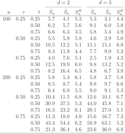
• Size of the tests under the null hypothesis H0:
– Table 1: Percentage of false rejections when data are serially independent. – Table 2: Percentage of false rejections when data are serially dependent.
• Power of the tests against specific alternatives:
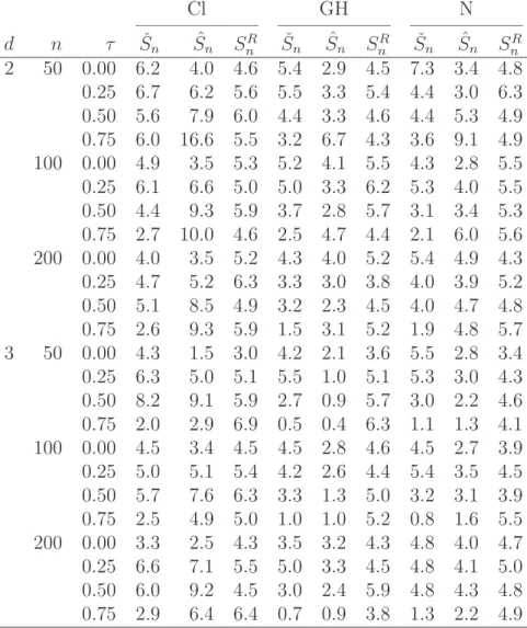
– Table 3: Power againstH0,m∩H1,c involving a change of the copula parameter
within a copula family and at serial independence.
– Table 4: Power against H0,m∩H1,c involving a change of copula family at a
constant value of Kendall’s tau and at serial independence.
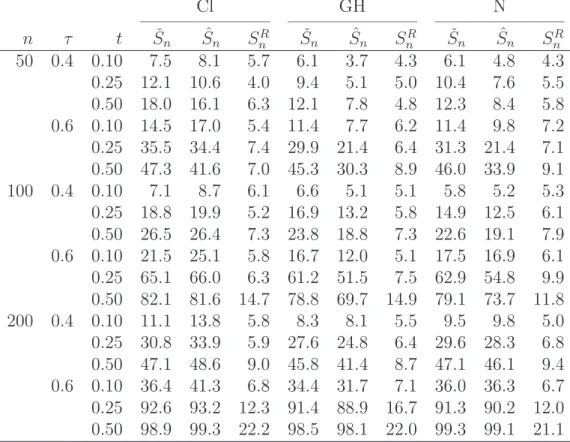
– Table 5: Power against H1,m∩H0,c involving a change in one of the margins
and at serial independence..
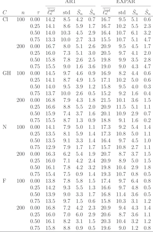
– Table 6: Power against ¬H0 when data are serially dependent and the change
occurs in the copula of the innovations.
Besides findings of a more anecdotical nature, the following conclusions may be drawn from the results:
• All tests hold their level reasonably well in the case of serial independence (Table 1), with minor fluctuations depending on sample size, test statistic, copula parameter and copula family.
• In case of serial dependence, the test based on ˆSnis too conservative for the sample sizes under consideration (Table 2). In line with this observation, the test based on
ˇ
Sn appears to be more powerful than the one based on ˆSn (Table 6).
• For alternative hypotheses involving a change in the copula, the tests based on ˆSn
and ˇSn have a higher power thanSR
n (Tables 3 and 4). When the copula changes in
such a way that Kendall’s tau remains constant, the power of SR
n is especially low.
With respect to that last setting, note that distinguishing copulas on the basis of low amounts of data is known to be difficult (Genest et al., 2009; Kojadinovic et al., 2011b). The fact that the change-point is unknown makes the problem even harder.
• For alternative hypotheses involving a change in one of the margins, it is the test statisticSR
n that is substantially more powerful thanSn(Table 5). The weak power
of Sn can be explained by the fact that it is designed for detecting changes in the copula. Another tentative reading of the results is that the test based on Sn, regarded as a procedure for testing H0,c, is relatively robust against small changes
in one margin. In contrast, the test based on SR
n behaves as an all-purpose test
for the hypothesis of a constant distribution rather than as a test for a constant copula.
6
Case studies
As an illustration, we first applied the test based on ˇSnto bivariate financial data consist-ing of daily logreturns computed from the DAX and the Standard and Poor 500 indices. Following Dehling et al. (2013, Section 7), attention was restricted to the years 2006– 2009. The corresponding closing quotes were obtained from http://quote.yahoo.com
using the get.hist.quote function of the tseries R package (Trapletti and Hornik, 2013), which resulted in n = 993 bivariate logreturns. Dependent multiplier sequences were generated as explained in Appendix C. An approximate p-value of 0.04 was obtained, providing some evidence against H0. The conclusion is in line with the results reported
in Dehling et al. (2013). Of course, as discussed earlier, it is only under the assumption thatH0,m in (1.2) holds that it would be fully justified to decide to rejectH0,c in (5.1) on
the basis of the previous approximate p-value. The value of the change- point estimator
k⋆
n in (2.5) is 529, corresponding to February 22nd, 2008.
As a second illustration, we followed again Dehling et al. (2013) and considered n = 504 bivariate logreturns computed from closing daily quotes of the Dow Jones Industrial Average and the Nasdaq Composite for the years 1987 and 1988. The former quotes, not being available on http://quote.yahoo.com anymore, were taken from the R package
QRM (Pfaff and McNeil, 2013). This two-year period is of interest because it contains October 19th, 1987, known as “black Monday” (see Dehling et al., 2013, Figure 4). An approximate p-value of 0.59 was obtained. Hence, despite the extreme events that oc-curred during the period under consideration, the test based on ˇSn detects no evidence againstH0 in the data, which is in line with the results reported in Dehling et al. (2013).
7
Conclusion
We have demonstrated that the sensitivity of rank-based tests for the null hypothesis of a constant distribution against changes in cross-sectional dependence can be improved if ranks are computed with respect to relevant subsamples. In this way, the test we propose achieves in many cases a higher power than the one proposed in B¨ucher and Ruppert (2013). The limit distribution of the test statistic under the null hypothesis is unwieldy, but approximate p-values can still be computed via a multiplier resampling scheme. To deal with potential serial dependence, we make use of dependent multiplier sequences, an idea going back to B¨uhlmann (1993) and revisited in B¨ucher and Kojadinovic (2013).
Here are some potential avenues for further research:
– Once the null hypothesis has been rejected, the nature of the nonstationary needs to be investigated further: is there a single change-point or is there more than one? Or maybe the change is gradual rather than sudden? And does the change concern the margins or the copula?
– Can one detect a change in the copula without the hypothesis that the margins are constant?
– The procedure is computationally intensive because the ranks have to be recomputed for every k ∈ {1, . . . , n−1}. Efficient algorithms for reutilizing calculations from one value ofk to the next one might speed up the computations.
Acknowledgments
The authors are grateful to Mark Holmes, Jean-Fran¸cois Quessy and Martin Ruppert for fruitful discussions, and to an anonymous referee for pointing out that Condition 3.1 might be dispensed with.
The research by A. B¨ucher has been supported in parts by the Collaborative Research Center “Statistical modeling of nonlinear dynamic processes” (SFB 823, Project A7) of the German Research Foundation (DFG), which is gratefully acknowledged.
J. Segers gratefully acknowledges funding by contract “Projet d’Actions de Recher-che Concert´ees” No. 12/17-045 of the “Communaut´e fran¸caise de Belgique” and by IAP research network Grant P7/06 of the Belgian government (Belgian Science Policy).
References
B. Auestad and D. Tjøstheim. Identification of nonlinear time series: First order charac-terization and order determination. Biometrika, 77:669–687, 1990.
J. Bai. Weak convergence of the sequential empirical processes of residuals in ARMA models. The Annals of Statistics, 22(4):2051–2061, 1994.
A. B¨ucher. A note on nonparametric estimation of bivariate tail de-pendence. Statistics and Risk Modeling, page in press, 2013a. URL
http://www.ruhr-uni-bochum.de/imperia/md/content/mathematik3/publications/taildep_buec
A. B¨ucher. A note on weak convergence of the sequential multivariate empirical process under strong mixing. Journal of Theoretical Probability, page in press, 2013b.
A. B¨ucher and H. Dette. A note on bootstrap approximations for the empirical copula process. Statistics and Probability Letters, 80(23–24):1925–1932, 2010.
A. B¨ucher and I. Kojadinovic. A dependent multiplier bootstrap for the sequential em-pirical copula process under strong mixing. arXiv:1306.3930, 2013.
A. B¨ucher and M. Ruppert. Consistent testing for a constant copula under strong mixing based on the tapered block multiplier technique. Journal of Multivariate Analysis, 116: 208–229, 2013.
A. B¨ucher and J. Segers. Extreme value copula estimation based on block maxima of a multivariate stationary time series. arXiv:1311.3060, 2013.
A. B¨ucher and S. Volgushev. Empirical and sequential empirical copula processes under serial dependence. Journal of Multivariate Analysis, 119:61–70, 2013.
P. B¨uhlmann. The blockwise bootstrap in time series and empirical processes. PhD thesis, ETH Z¨urich, 1993. Diss. ETH No. 10354.
M. Cs¨org˝o and L. Horv´ath. Limit theorems in change-point analysis. Wiley Series in Probability and Statistics. John Wiley & Sons, Chichester, UK, 1997.
H. Dehling, D. Vogel, M. Wendler, and D. Wied. An efficient and robust test for a change-point in correlation. arXiv:1203.4871, 2013.
C. Genest and J. Segers. On the covariance of the asymptotic empirical copula process.
Journal of Multivariate Analysis, 101:1837–1845, 2010.
C. Genest, K. Ghoudi, and L.-P. Rivest. Discussion of “Understanding relationships using copulas”, by E. Frees and E. Valdez. North American Actuarial Journal, 3:143–149, 1998.
C. Genest, B. R´emillard, and D. Beaudoin. Goodness-of-fit tests for copulas: A review and a power study. Insurance: Mathematics and Economics, 44:199–213, 2009.
E. Gombay and L. Horv´ath. Change-points and bootstrap. Environmetrics, 10(6), 1999. E. Gombay and L. Horv´ath. Rates of convergence for U-statistic processes and their bootstrapped versions. Journal of Statistical Planning and Inference, 102:247–272, 2002.
M. Hofert, I. Kojadinovic, M. M¨achler, and J. Yan. copula: Multivariate dependence with copulas, 2013. URL http://CRAN.R-project.org/package=copula. R package version 0.999-7.
M. Holmes, I. Kojadinovic, and J-F. Quessy. Nonparametric tests for change-point de-tection `a la Gombay and Horv´ath. Journal of Multivariate Analysis, 115:16–32, 2013. A. Inoue. Testing for distributional change in time series. Econometric Theory, 17(1):
156–187, 2001.
A. Khoudraji. Contributions `a l’´etude des copules et `a la mod´elisation des valeurs extrˆemes bivari´ees. PhD thesis, Universit´e Laval, Qu´ebec, Canada, 1995.
I. Kojadinovic. npcp: Some nonparametric tests for change-point detection in (multi-variate) observations, 2014. URL http://CRAN.R-project.org/package=npcp. R package version 0.0-1.
I. Kojadinovic, J. Segers, and J. Yan. Large-sample tests of extreme-value dependence for multivariate copulas. The Canadian Journal of Statistics, 39(4):703–720, 2011a. I. Kojadinovic, J. Yan, and M. Holmes. Fast large-sample goodness-of-fit for copulas.
Statistica Sinica, 21(2):841–871, 2011b.
E. Liebscher. Construction of asymmetric multivariate copulas. Journal of Multivariate Analysis, 99:2234–2250, 2008.
E. Paparoditis and D.N. Politis. Tapered block bootstrap. Biometrika, 88(4):1105–1119, 2001.
B. Pfaff and A. McNeil. QRM: Provides R-language Code to Examine Quantitative Risk Management Concepts, 2013. URL http://CRAN.R-project.org/package=QRM. R package version 0.4-9.
J.-F. Quessy, M. Sa¨ıd, and A.-C. Favre. Multivariate Kendall’s tau for change-point detection in copulas. The Canadian Journal of Statistics, 41:65–82, 2013.
R Development Core Team. R: A Language and Environment for Statistical Com-puting. R Foundation for Statistical Computing, Vienna, Austria, 2013. URL
http://www.R-project.org. ISBN 3-900051-07-0.
B. R´emillard. Goodness-of-fit tests for copulas of multivariate time series. Social Science Research Network, 1729982:1–32, 2010. URLhttp://ssrn.com/abstract=1729982. B. R´emillard and O. Scaillet. Testing for equality between two copulas. Journal of
Multivariate Analysis, 100(3):377–386, 2009.
J.P. Romano and M. Wolf. A more general central limit theorem form-dependent random variables with unbounded m. Statistics and Probability Letters, 47:115–124, 2000. O. Scaillet. A Kolmogorov-Smirnov type test for positive quadrant dependence.Canadian
Journal of Statistics, 33:415–427, 2005.
J. Segers. Asymptotics of empirical copula processes under nonrestrictive smoothness assumptions. Bernoulli, 18:764–782, 2012.
A. Sklar. Fonctions de r´epartition `a n dimensions et leurs marges. Publications de l’Institut de Statistique de l’Universit´e de Paris, 8:229–231, 1959.
A. Trapletti and K. Hornik. tseries: Time series analysis and computational finance, 2013. URLhttp://CRAN.R-project.org/package=tseries. R package version 0.10-32.
A.W. van der Vaart and J.A. Wellner. Weak convergence and empirical processes. Springer, New York, 2000. Second edition.
M. van Kampen and D. Wied. A nonparametric constancy test
for copulas under mixing conditions. working paper, 2013. URL
D. Wied, H. Dehling, M. van Kampen, and D. Vogel. A fluctuation test for constant Spearman’s rho with nuisance-free limit distribution. Computational Statistics and Data Analysis, page in press, 2013.
A
Proof of Proposition 3.3
Let us first introduce additional notation. For integers 1≤k ≤l≤n, let Hk:l denote the
empirical c.d.f. of the unobservable sample Uk, . . . ,Ul and let Hk:l,j, for j ∈ {1, . . . , d},
denote its margins. The empirical quantile functions are
Hk−:l,j1 (u) = inf{v ∈[0,1] :Hk:l,j(v)≥u}, u∈[0,1],
which are collected in a vector via
H−1 k:l(u) = H −1 k:l,1(u1), . . . , H −1 k:l,d(ud) , u ∈[0,1]d.
By convention, the previously defined quantities are all taken equal to zero if k > l. From the proof of Theorem 3.4 in B¨ucher and Kojadinovic (2013), we have that (3.6) holds with Cn replaced by Calt
n , where Calt n (s, t,u) = 1 √ n ⌊nt⌋ X i=⌊ns⌋+1 [1{Ui ≤H−1 ⌊ns⌋+1:⌊nt⌋(u)} −C(u)], (s, t,u)∈∆×[0,1] d.
To show (3.6), it remains therefore to prove that sup (s,t,u)∈∆×[0,1]d Caltn (s, t,u)−Cn(s, t,u) P →0. (A.1)
To do so, we adapt the arguments used in Lemma A.2 of B¨ucher and Segers (2013). Fix 1 ≤ k ≤ l ≤ n and u ∈ [0,1]d. For i ∈ {k, . . . , l}, the d components of ˆUk:l
i defined
in (2.2) can be expressed as ˆUk:l
ij =Hk:l,j(Uij), j ∈ {1, . . . , d}. Next, notice that
1 Uij ≤Hk−:l,j1 (uj) −1 Uˆijk:l ≤uj =1 Uij < Hk−:l,j1 (uj) +1 Uij =Hk−:1l,j(uj) −1 Uˆk:l ij < uj −1 Uˆk:l ij =uj =1 Uij =Hk−:l,j1 (uj) −1 Uˆijk:l =uj ,
as x < H−1(u) if and only H(x) < u for any distribution function H. Since ˆUk:l ij = Hk:l,j(Uij) =uj implies Uij =Hk−:1l,j(uj), we obtain that
0≤1
Uij ≤Hk−:l,j1 (uj) −1 Uˆijk:l ≤uj
≤1
Uij =Hk−:1l,j(uj) .
Combining the previous inequality with the decomposition 1{Ui ≤H−1 k:l(u)} −1( ˆUik:l ≤u) = d X p=1 " Y 1≤j≤p 1{Uij ≤Hk−:l,j1 (uj)} Y p<j≤d 1( ˆUijk:l≤uj) − Y 1≤j≤p−1 1{Uij ≤Hk−:1l,j(uj)} Y p−1<j≤d 1( ˆUijk:l≤uj) # ,
we obtain that 0≤1{Ui ≤H−1 k:l(u)} −1( ˆUik:l ≤u)≤ d X j=1 1 Uij =Hk−:l,j1 (uj) . (A.2)
It follows that the supremum in (A.1) is smaller than
d X j=1 sup (s,t,u)∈∆×[0,1] 1 √ n ⌊nt⌋ X i=⌊ns⌋+1 1 Uij =H⌊−ns1⌋+1:⌊nt⌋,j(u) ≤ d X j=1 sup u∈[0,1] 1 √ n n X i=1 1(Uij =u).
Using the fact that 1 Uij =u
≤1 Uij ≤u
−1 Uij ≤u−1/n
, the latter is smaller
d sup
u,v∈[0,1]d
ku−vk1≤n−1
|Bn(0,1,u)−Bn(0,1,v)|+dn−1/2,
where Bn is defined in (3.4). Using the asymptotic uniform equicontinuity in probability
ofBnestablished in Lemma 2 of B¨ucher (2013b), we finally obtain (A.1), which completes
the proof.
B
Proof of Proposition 4.3
We shall only prove the result in the case of strongly mixing observations, that is, when Condition 4.1(ii) is assumed. The proof is similar but simpler when Condition 4.1(i) is assumed instead.
It is sufficient to show the statement involving ˇC(nm). The statements for ˇD(nm) and
ˇ
Sn(m) then follow from the continuous mapping theorem.
For any m∈ {1, . . . , M} and (s, t,u)∈∆×[0,1]d, put
B(m) n (s, t,u) = 1 √ n ⌊nt⌋ X i=⌊ns⌋+1 ξi,n(m){1(Ui ≤u)−C(u)}, (B.1) C(m) n (s, t,u) = B(nm)(s, t,u)− d X j=1 ˙ Cj(u)B(m) n (s, t,u(j)).
[Recall that u(j) = (1, . . . ,1, uj,1, . . . ,1) ∈[0,1]d, with uj appearing at the j-th
coordi-nate.] From Theorem 2.1 in B¨ucher and Kojadinovic (2013), we have that
Bn,B(1) n , . . . ,B(nM) B C,B(1)C , . . . ,B(CM) in{ℓ∞(∆×[0,1]d)}M+1, where B(1) C , . . . ,B (M)
C are independent copies of BC in (3.5), and
thus, from the continuous mapping theorem and (3.6), we find that
Cn,C(1) n , . . . ,C(nM) CC,C(1) C , . . . ,C (M) C
in {ℓ∞(∆×[0,1]d)}M+1. It is therefore sufficient to show that sup (s,t,u)∈∆×[0,1]d ( ˇC(nm)−C(nm))(s, t,u) P →0 (B.2)
for every m∈ {1, . . . , M}. Below, we will show the following two assertions: first, sup (s,t,u)∈∆×[0,1]d (ˇB(nm)−B(nm))(s, t,u) P →0, (B.3)
and second, for every δ∈(0,1/2) and every ε∈(0,1), sup u∈[0,1]d δ≤uj≤1−δ sup (s,t)∈[0,1]2 t−s≥ε Cj,˙ ⌊ns⌋+1:⌊nt⌋(u)−Cj˙ (u) P →0. (B.4)
In view of the structure of ˇC(nm) in (4.3), the assertions (B.3) and (B.4) imply (B.2), as
we show next. Clearly,
( ˇC(nm)−C(nm))(s, t,u) ≤ (ˇB(nm)−B(nm))(s, t,u) + d X j=1 C˙j,⌊ns⌋+1:⌊nt⌋(u) (ˇB(nm)−Bn(m))(s, t,u(j)) + d X j=1 Cj,˙ ⌊ns⌋+1:⌊nt⌋(u)−Cj˙ (u) B(nm)(s, t,u(j)) . (B.5)
Taking suprema over (s, t,u)∈∆×[0,1]d, the first and the second term on the right-hand
side of (B.5) converge to zero in probability because of assertion (B.3) and uniform bound-edness of ˙Cj,k:l(see Kojadinovic et al., 2011a, proof of Proposition 2). The third term on
the right-hand side of (B.5) converges to zero in probability because of assertion (B.4) and the fact that (s, t,u)7→B(nm)(s, t,u(j)) vanishes as soon ass=toruj ∈ {0,1}, and is
asymptotically uniformly equicontinuous in probability as a consequence of Lemma A.3 in B¨ucher and Kojadinovic (2013).
It remains to show (B.3) and (B.4). The proof of the latter assertion is simplest and is given first.
Proof of (B.4). Observe that
C⌊ns⌋+1:⌊nt⌋(u) =C(u) +
1
√
n λn(s, t)Cn(s, t,u).
Fixδ ∈(0,1/2) andε∈(0,1). Without loss of generality, assume that n is large enough so that the bandwidth h=hn(s, t) = 1/p⌊nt⌋ − ⌊ns⌋ is less than δ whenever t−s≥ε. Then, for t−s≥ε and u∈[0,1]d with δ≤uj ≤1−δ, we have
˙ Cj,⌊ns⌋+1:⌊nt⌋(u) = 1 2h{C(u+hej)−C(u−hej)} + 1 2h√n λn(s, t){Cn(s, t,u+hej)−Cn(s, t,u−hej)}.
By the assumption of existence and continuity of ˙Cj onVj (see Condition 3.2), and since 0≤Cj˙ ≤1, it follows from the mean-value theorem that
sup u∈[0,1]d δ≤uj≤1−δ 1 2h{C(u+hej)−C(u−hej)} −Cj˙ (u) → 0, h→0.
Using (3.6) and the fact thatBnis asymptotically uniformly equicontinuous in probability,
it can be verified that Cn is asymptotically uniformly equicontinuous in probability as
well. It follows that sup u∈[0,1]d δ≤uj≤1−δ sup (s,t)∈[0,1]2 t−s≥ε Cn(s, t,u+hej)−Cn(s, t,u−hej) P →0. Finally, 1 2h√n λn(s, t) = 1 2pλn(s, t) ≤ 1 2pε−1/n.
Combine the four previous displays to arrive at the desired conclusion.
The proof of (B.3) is more complicated. Using the notation introduced in Appendix A, let us define the auto-centered version of the process B(nm) in (B.1) as
˚B(m) n (s, t,u) = 1 √ n ⌊nt⌋ X i=⌊ns⌋+1 ξi,n(m){1(Ui ≤u)−H⌊ns⌋+1:⌊nt⌋(u)} = √1 n ⌊nt⌋ X i=⌊ns⌋+1 (ξ(i,nm)−ξ¯⌊(mns)⌋+1:⌊nt⌋)1(Ui ≤u), (B.6)
with the usual convention that empty sums are zero.
Proof of (B.3). Consider the decomposition
(ˇB(nm)−B(nm))(s, t,u) ≤ Bˇ(nm)(s, t,u)−˚Bn(m)(s, t,H⌊−ns1⌋+1:⌊nt⌋(u)) + ˚B(nm)(s, t,H⌊−ns1⌋+1:⌊nt⌋(u))−B(nm)(s, t,H⌊−ns1⌋+1:⌊nt⌋(u)) + B(nm)(s, t,H⌊−ns1⌋+1:⌊nt⌋(u))−B(nm)(s, t,u) .
Write out the definitions of the processes B(nm), ˚Bn(m) and ˇB(nm) in (B.1), (B.6) and (4.2),
respectively, and take suprema over (s, t,u)∈∆×[0,1]d to obtain
sup (s,t,u)∈∆×[0,1]d (ˇB(nm)−B(nm))(s, t,u) ≤ sup (s,t,u)∈∆×[0,1]d Bˇ(nm)(s, t,u)−˚Bn(m)(s, t,H⌊−ns1⌋+1:⌊nt⌋(u)) (B.7) + sup (s,t,u)∈∆×[0,1]d 1 √n ⌊nt⌋ X i=⌊ns⌋+1 ξi,n(m) H⌊ns⌋+1:⌊nt⌋(u)−C(u) (B.8) + sup (s,t,u)∈∆×[0,1]d B(nm)(s, t,H⌊−ns1⌋+1:⌊nt⌋(u))−B(nm)(s, t,u) . (B.9)
1- The term (B.8): Let δ ∈ (0,1/2), to be specified later. We split the supremum into two parts, according to whether t−s is smaller or larger thanan =n−1/2−δ:
An,1 = sup (s,t,u)∈∆×[0,1]d t−s≤an 1 √ n ⌊nt⌋ X i=⌊ns⌋+1 ξi,n(m) H⌊ns⌋+1:⌊nt⌋(u)−C(u) , An,2 = sup (s,t,u)∈∆×[0,1]d t−s≥an 1 √ n ⌊nt⌋ X i=⌊ns⌋+1 ξi,n(m) H⌊ns⌋+1:⌊nt⌋(u)−C(u) .
We will show that both An,1 and An,2 converge to zero in probability.
(a) Since both Hk:l and C take values in [0,1], a crude bound forAn,1 is
An,1 ≤
1
√
n(n an+ 1) max1≤i≤n|ξ
(m)
i,n | ≤2n−δ 1max≤i≤n|ξi,n|.
Using the fact that, from (M1), for any ν ≥ 1, supn≥1E[|ξ (m)
1,n|ν] < ∞, we have
that, for every α >0 andν ≥1 such that ν > 1/α, P max 1≤i≤n|ξ (m) i,n | ≥nα ≤nP |ξ(1m,n)| ≥nα ≤n1−να E[|ξ1(m,n)|ν]→0.
Apply the previous display with α ∈ (0, δ) to find that An,1 converges to zero in
probability.
(b) Recall Bn in (3.4). Observe that
Bn(s, t,u) = ⌊nt⌋ − ⌊√ ns⌋ n {H⌊ns⌋+1:⌊nt⌋(u)−C(u)}. We have An,2 = sup (s,t,u)∈∆×[0,1]d t−s≥an 1 ⌊nt⌋ − ⌊ns⌋ ⌊nt⌋ X i=⌊ns⌋+1 ξi,n(m) Bn(s, t,u) ≤ sup ⌊ns⌋<⌊nt⌋ ⌊nt⌋+1−⌊ns⌋≥nan 1 ⌊nt⌋ − ⌊ns⌋ ⌊nt⌋ X i=⌊ns⌋+1 ξi,n(m) sup (s,t,u)∈∆×[0,1]d Bn(s, t,u) ≤ max 1≤k≤l≤n l−k≥nan 1 l−k+ 1 l X i=k ξ(i,nm) sup (s,t,u)∈∆×[0,1]d Bn(s, t,u) .
By weak convergence Bn BC in ℓ∞(∆ ×[0,1]d), the supremum at the end of
the previous display is bounded in probability. Writing bn = nan, it is sufficient to show that max 1≤k≤l≤n l−k≥bn 1 l−k+ 1 l X i=k ξi,n(m) P →0, n → ∞.
Fixη >0. The probability that the previous maximum exceeds η is bounded by X 1≤k≤l≤n l−k≥bn P 1 l−k+ 1 l X i=k ξi,n(m) > η . (B.10)
Fix ν ≥ 2, to be specified later. By stationarity and Markov’s inequality, the previous expression is bounded by
X 1≤k≤l≤n l−k≥bn η−ν(l−k+ 1)−ν E l−k+1 X i=1 ξi,n(m) ν ≤η−νn X bn≤r≤n r−ν E r X i=1 ξ(i,nm) ν .
Recall that the sequence (ξi,n(m))i∈Z isℓn-dependent from (M2) and assume thatnis sufficiently large so thatn ≥2ℓn+bn. Then, by Corollary A.1 in Romano and Wolf (2000), there exists a constant Cν, depending only on ν, such that
E r X i=1 ξi,n(m) ν ≤Cνν(4ℓnr)ν/2 E[|ξ1(m,n)|ν].
Using the fact that, from (M1), supn≥1E[|ξ1(,nm)|ν]<∞, and up to a multiplicative
constant, the expression in (B.10) is bounded by
n X bn≤r≤n r−ν(ℓnr)ν/2 ≤n2b−nν/2ℓν/n 2 =O n2−(1/2−δ)ν/2+(1/2−γ)ν/2 =O n2+(δ−γ)ν/2 .
The right-hand side converges to zero if we chooseδ=γ/2 and then ν >8/γ. 2- The term (B.9): We have to show that, for every η, λ >0,
P " sup (s,t,u)∈∆×[0,1]d B(nm){s, t,H⌊−ns1⌋+1:⌊nt⌋(u)} −B(nm)(s, t,u) > λ # ≤η,
for all sufficiently large n.
Fix η, λ > 0. Since (B.9) is smaller than 2 sup(s,t,u)∈∆×[0,1]d|B
(m)
n (s, t,u)|, and using
the fact that B(nm) vanishes on the diagonal s = t and is asymptotically uniformly
equicontinuous in probability, there exists ε ∈ (0,1) such that, for all n sufficiently large, P sup (s,t,u)∈∆×[0,1]d t−s<ε B(nm){s, t,H⌊−ns1⌋+1:⌊nt⌋(u)} −B(nm)(s, t,u) > λ ≤η/2.
Setting ζn = sup(s,t,u)∈∆×[0,1]d t−s≥ε k
H−1
⌊ns⌋+1:⌊nt⌋(u)−uk1, we shall now show that, for alln
sufficiently large, An= P sup (s,t,u,v)∈∆×[0,1]2d t−s≥ε,ku−vk1≤ζn B(nm)(s, t,u)−B(nm)(s, t,v) > λ ≤η/2,
which will complete the proof. Using again the asymptotic uniformly equicontinuity in probability of B(nm), there exists µ∈(0,1) such that, for all n sufficiently large,
An,1 = P sup (s,t,u,v)∈∆×[0,1]2d t−s≥ε,ku−vk1≤µ B(nm)(s, t,u)−B(nm)(s, t,v) > λ ≤η/4.
We then boundAnbyAn,1+An,2, whereAn,2 = P(ζn> µ). From the weak convergence
of Bn toBC inℓ∞(∆×[0,1]d), we have that sup (s,t,u)∈∆×[0,1]d t−s≥ε |H⌊ns⌋+1:⌊nt⌋(u)−C(u)| ≤ sup (s,t,u)∈∆×[0,1]d |Bn(s, t,u)| ×n−1/2× sup (s,t)∈∆ t−s≥ε {λn(s, t)}−1 P→0.
Using the fact that supu∈[0,1]|H⌊ns⌋+1:⌊nt⌋,j(u)−u|= supu∈[0,1]|H⌊−ns1⌋+1:⌊nt⌋,j(u)−u| for j ∈ {1, . . . , d} (for instance, by symmetry arguments on the graphs of H⌊ns⌋+1:⌊nt⌋,j
and H⌊−ns1⌋+1:⌊nt⌋,j), we immediately obtain that ζn →P 0, which implies that, for all n
sufficiently large, An,2 ≤η/4, and thus that, for all n sufficiently large, An ≤η/2.
3- The term (B.7): For the following arguments, it is sufficient to assume that the sequence (ξ(i,nm))i∈Z appearing in ˇB(nm) and ˚B(nm) satisfies only (M1) with E[{ξ0(,nm)}2]>0
not necessarily equal to one.
LetK >0 be a constant and let us first suppose that, for anyn ≥1 andi∈ {1, . . . , n},
ξi,n(m) ≥ −K. With (A.2) in mind, the term (B.7) is smaller thanAn,1+An,2, where
An,1 = sup (s,t,u)∈∆×[0,1]d 1 √ n ⌊nt⌋ X i=⌊ns⌋+1 (ξi,n(m)+K)h1{Ui ≤H−1 ⌊ns⌋+1:⌊nt⌋(u)} −1( ˆU ⌊ns⌋+1:⌊nt⌋ i ≤u) i and An,2 = sup (s,t,u)∈∆×[0,1]d K+ ¯ξ⌊(mns)⌋+1:⌊nt⌋ √ n ⌊nt⌋ X i=⌊ns⌋+1 h 1{Ui ≤H−1 ⌊ns⌋+1:⌊nt⌋(u)} −1( ˆU ⌊ns⌋+1:⌊nt⌋ i ≤u) i .
Let us first show that An,1 P
→0. Plugging (A.2) into the expression ofAn,1, we bound
An,1 by An,1,1+· · ·+An,1,d, where An,1,j = sup (s,t,u)∈∆×[0,1] 1 √n ⌊nt⌋ X i=⌊ns⌋+1 (ξi,n(m)+K)1 Uij =u .