Limitations and Potential of Complex Cloud Analysis and Its Improvement for Radar Reflectivity Data Assimilation Using OSSEs.

(1)

UNIVERSITY OF OKLAHOMA GRADUATE COLLEGE

LIMITATIONS AND POTENTIAL OF COMPLEX CLOUD ANALYSIS AND ITS IMPROVEMENT FOR RADAR REFLECTIVITY DATA ASSIMILATION

USING OSSES

A DISSERTATION

SUBMITTED TO THE GRADUATE FACULTY in partial fulfillment of the requirements for the

Degree of DOCTOR OF PHILOSOPHY By CHONG-CHI TONG Norman, Oklahoma 2015

(2)

LIMITATIONS AND POTENTIAL OF COMPLEX CLOUD ANALYSIS AND ITS IMPROVEMENT FOR RADAR REFLECTIVITY DATA ASSIMILATION

USING OSSES

A DISSERTATION APPROVED FOR THE SCHOOL OF METEOROLOGY

BY

______________________________ Dr. Ming Xue, Chair

______________________________ Dr. David Parsons ______________________________ Dr. Fanyou Kong ______________________________ Dr. Guifu Zhang ______________________________ Dr. Lance Leslie ______________________________ Dr. Sivaramakrishnan Lakshmivarahan

(3)

(4)

Acknowledgements

It has been such a long journey finishing up a doctoral degree! Achievement like this can’t be done without continuous passion, which could be supported and refilled by a number of wonderful people: Dr. Ming Xue, my advisor, who kept five years of regular meetings in which I obtained inspiring and valuable instructions on my research, my other committee members, Drs. David Parsons, Lance Leslie, Fanyou Kong, Guifu Zhang, and S. Lakshmivarahan, who helped me refine my dissertation research with helpful suggestions and greatest patience, and those professors who taught the classes from which I acquired useful knowledge and skills highly beneficial to my Ph.D. works. In addition, I want to appreciate the hard-working research crew who kept developing and maintaining the ARPS system. Thanks to Drs. Keith Brewster and Youngsun Jung for their helps on resolving some technical problems. My classmates and colleagues, Bryan Putnam, Rong Kong, Gang Zhao, Mike VandenBerg, and Jonty Hall are thanked for the inspiring discussions on course or research works. I also appreciate the warm cares and administrative assistance provided by the kind secretaries in both the CAPS and SoM, including Ms. Eileen Hasselwander, Debra Farmer, Christie Upchurch, and Celia Jones. Mutual cheering-ups provided by the forever-enthusiastic-Thunder-fan, Marcia Pallutto with relaxation from my intense study are truly valued.

Last, I would like to save some space for my loving and beloved family, especially my parents, grandparents, and my sister. Thanks for them to bear this long-term separation with their endless support and encouragement for me to pursue my study-abroad dream. Deepest love will be for them like always!

(5)

The simulation works presented in this study were performed using the supercomputing resources provided by the Extreme Science and Engineering Discovery Environment (XSEDE) and OU Supercomputing Center for Research and Education (OSCER).

(6)

List of Tables

Table 1.1 Summary of the differences between Ge et al. (2013) and this study ... 6

Table 2.1 Summary ARPS complex cloud analysis procedure ... 18

Table 2.2 Empirical hard thresholds used to suppress apparently wrong designations (reproduced from Park et al. 2009) ... 24

Table 2.3 Naming of experiments with corresponding settings ... 29

Table 3.1 List of the truth simulation, four smoothing experiments, and their respective statistics ... 48

Table 3.2 Configurations of microphysics experiments ... 60

Table 3.3 Configurations of direct insertion experiments ... 76

(10)

List of Figures

FIG. 1.1 Equitable threat score (ETS) of hourly precipitation at 0.5 inch threshold averaged over the last 15 days of 2008 Spring Experiment. Experiments with grid spacing of 4 km and 2 km are denoted by blue and red color, respectively. Dash line indicates experiment with no radar analysis. Adapted from Xue et al. (2008). ... 4 FIG. 2.1 Trapezoidal membership function, where X is an arbitrary radar variable. Adapted from Park et al. (2009). ... 23 FIG. 2.2 Weekly averaged sea surface temperature during 2-8 June 2008 and MCV track. Gray dots and black dots are tracked by IR satellite images and radar radial velocity, respectively. Red square denotes the domain of our simulation. Reproduced from Lai et al. (2011). ... 27 FIG. 2.3 Distribution of four CWB operational radars and NCAR S-Pol radar. Observing ranges are denoted by circles in corresponding colors (200 km for CWB radars and 150 km for NCAR S-Pol). ... 28 FIG. 2.4 (a) Composite reflectivity observed by NCAR S-Pol at 00 UTC 5 June 2008 and a (b) selected cross section . ... 29 FIG. 2.5 Mixing ratio (g/kg) analyses for hydrometeor: (a)(b) rain, (c)(d) snow, and (e)(f) hail, using KRY (left panel) and JZX (right panel) procedure. ... 31 FIG. 2.6 Hourly rainfall accumulation (mm) of (a) CWB QPESUMS, (b) KRY_S, (c) JZX_S, (d) KRY_D, and (e) JZX_D valid at 01 UTC 5 June 2008. Hour rainfall maximum is written at the lower right corner of each plot. ... 35

(11)

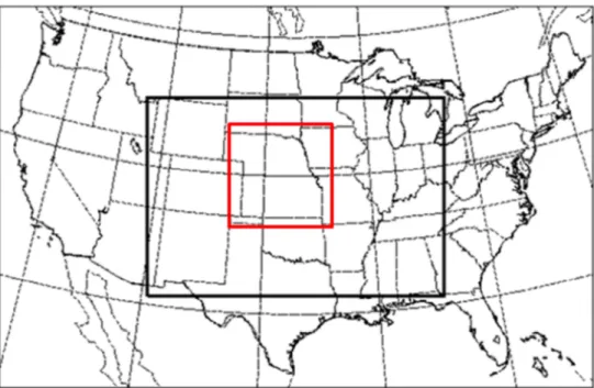
FIG. 2.7 One hour forecast of mixing ratio (g/kg) analyses for hydrometeor: (a)(b) rain, (c)(d) snow, and (e)(f) hail of experiment KRY_S (left panel) and JZX_S (right panel). ... 36 FIG. 3.1 Synoptic analysis at 925 mb valid at 00 UTC 19 May 2013. Geopotential height, temperature, and dew point temperature are provided with black solid contours, red dash contours, and green solid contours, respectively. Winds are provided in flags. Courtesy to the Storm Prediction Center of NOAA’s National Weather Service. ... 42 FIG. 3.2 Computational domains used for the experimental EnKF ensemble in 2013 Spring Experiment (600 × 400 grids with 4-km spacing denoted by black rectangle) and our study (803 × 803 grids with 1-km spacing denoted by red square). ... 44 FIG. 3.3 Time line of the truth simulation and the experiments. Main studied period is marked by gray shading area. ... 45 FIG. 3.4 Hourly simulated composite reflectivity (Z) and surface winds (Vh) of the truth

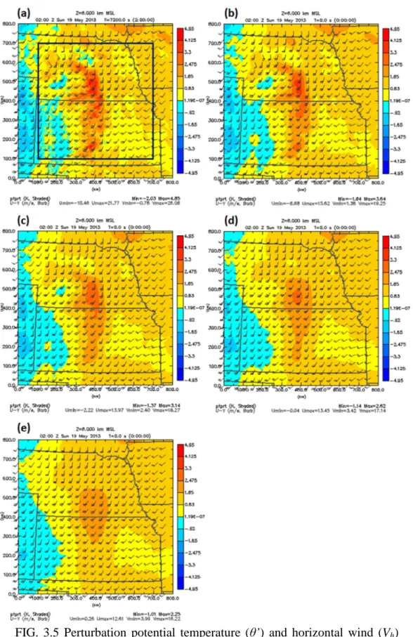
simulation at (a) 02 UTC, (b) 03 UTC, (c) 04 UTC, (d) 05 UTC, and (e) 06 UTC. Wind flags are plotted in 40 km interval. ... 46 FIG. 3.5 Perturbation potential temperature (θ’) and horizontal wind (Vh) field at 6 km

AGL at 02 UTC for (a) the truth simulation, experiment (b) SMT_d15, (c) SMT_d35, (d) SMT_d55, and (e) SMT_d75. Wind flags are plotted in 40 km interval. ... 49

(12)

FIG. 3.6 SRMS error time series of (a) Vh, (b) w, (c) T, (d) qv, (e) qw, and (f) all

variables for four smoothing experiments. The extra gray solid line in (b) is for a

uniform 0 m s-1 w field. ... 52

FIG. 3.7 (a) RMS_Z, (b) bias score, and (c) ETS calculated with threshold of 30 dBZ for four smoothing experiments. ... 54

FIG. 3.8 Same as FIG.3.4, but for the experiment SMT_d15. ... 55

FIG. 3.9 Same as FIG. 3.4, but for the experiment SMT_d75. ... 56

FIG. 3.10 ASED of four smoothing experiments. ... 58

FIG. 3.11 Same as FIG. 3.6, but for the CNTL and three microphysics experiments. .. 62

FIG. 3.12 Same as 3.10, but for the CNTL and three microphysics experiments. ... 64

FIG. 3.13 Composite reflectivity and surface winds at 02 UTC for (a) truth simulation, (b) CNTL, (c) MYSM, (d) MYDM, and (e) Lin. The convergent line is indicated by a red dash line in (a). Wind arrows are plotted in 30 km interval. ... 68

FIG. 3.14 Same as FIG. 3.13, but for 04 UTC. ... 69

FIG. 3.15 Same as FIG. 3.7, but for the CNTL and three microphysics experiments. .. 72

FIG. 3.16 Same as FIG. 3.6, but for the CNTL and five direct insertion experiments. . 81

FIG. 3.17 Same as FIG. 3.7, but for the CNTL and five direct insertion experiments. . 84

FIG. 3.18 Composite reflectivity and surface winds at 03 UTC for (a) Pt, (b) Qv, (c) Qcld, (d) Qpcp, and (e) Qall. Wind arrows are plotted in 30 km interval. ... 85

FIG. 4.1 Cross section of truth mixing ratio in g kg-1 for (a) rain water, (b) snow, (c) graupel, and (d) hail. ... 93

(13)

FIG. 4.3 Cross section of 10log(N0) from the truth simulation for (a) rain, (b) snow, and

(c) graupel. The default N0 values are marked by black dash line on the color bar.

... 97 FIG. 4.4 Composite reflectivity and surface winds at 2:00 UTC for (a) truth simulation and (b) experiments with cloud analysis. ... 98 FIG. 4.5 Same as FIG. 3.6, but for the CNTL and four cloud analysis experiments. .... 98 FIG. 4.6 Same as 3.10, but for the CNTL and four cloud analysis experiments. ... 103 FIG. 4.7 Same as FIG. 3.7, but for the CNTL and four cloud analysis experiments. .. 105 FIG. 4.8 Same as FIG. 3.18, but for four cloud analysis experiments (a) NoAdj, (b) PtAdj, (c) QvAdj, and (d) BothAdj. ... 107 FIG. 4.9 Conceptual model of the forecast error evolution corresponding to IC accuracy (including the resolution fineness of moisture field and hydrometeor availability) and model perfectness. Details about the arrow marks are provided in the context. ... 111 FIG. 5.1 Cross section of RH field (%) for (a) truth simulation, (b) background (CNTL), and (d) QvAdj. The RH difference between the truth and CNTL (CNTL-truth) is given as (c). The height of 0 °C is denoted by white solid lines in (a) and (b). 15 dBZ echo boundary is drawn by gray contour in (c) and (d) for a rough illustration of cloudy regions. The LCL is denoted by a blue dash line in (d). 120 FIG. 5.2 RMS error of qv as a function of height (in terms of model level) at forecast

initial (2:00 UTC). Experiments with and without hydrometeor analysis are represented by solid and dash lines, respectively. The ninth level is marked with a horizontal blue dash line. See context for detailed description. ... 122

(14)

FIG. 5.3 Cross section of RH field (%) for (a) truth simulation and (c) RHInsrt. Cross section of qv field (g/kg) for (b) truth simulation and (d) RHInsrt. Corresponding

0 °C levels are denoted by white solid lines. 15 dBZ echo boundary is drawn by gray contour. The LCL is denoted by blue dash line for experiment RHInsrt indicating the bottom boundary of adjustment. ... 125 FIG. 5.4 Same as FIG. 3.6, but for the CNTL, TrueQv, NoAdj, SatAdj, RHInsrt, and UpdftAdj. ... 126 FIG. 5.5 RMS error of (a) u, (b) θ, (c) qv, and (d) qw as a function of height (in terms of

model level) at 30-min forecast (2:30 UTC). Experiments with and without hydrometeor analysis are represented by solid and dash lines, respectively. ... 130 FIG. 5.6 Same as FIG. 3.7, but for the CNTL, TrueQv, NoAdj, SatAdj, RHInsrt, and UpdftAdj. ... 132 FIG. 5.7 Same as FIG. 5.1a, but with black contours of true w = -0.2 m/s overlaid. ... 133 FIG. 5.8 Diagram of w and RH fields used for statistics above the FL. Area within the blue and black ellipses denotes w < threshold and RH < 100%, respectively. Hits and misses corresponding to the contingency table test (Table 5.1) are shaded in gray and yellow color, respectively. ... 135 FIG. 5.9 HMR as a function of varying w threshold. ... 136 FIG. 5.10 SRMSE of qv as a function of varying constant RH value specified for

negative w areas. For reference purpose, SRMSEs of some other associated experiments are listed at upper right corner of the plot. ... 138

(15)

FIG. 5.11 Scatter plot of the true w and RH within the cloudy regions below the FL. Scatters between two black dash lines are used to fit for polynomial relations. Blue curve is the final relation used as the modified qv adjustment. ... 141

FIG. 5.12 Retrieval of w-RH relationship using (a) first order, (b) second order, and (c) third order polynomial regression. Regression results are plotted with blue solid line or curves in the middle of the figures, along with the equations written. Constant RH values used for w exceeding terminal thresholds are marked with horizontal dashed blue lines at both sides. SRMS error of qv analysis using

corresponding equation is listed at the bottom left corner of each plot. ... 142 FIG. 5.13 Same as FIG. 5.3, but for the SatAdj (upper panel) and UpdftAdj (lower panel). ... 144

(16)

Abstract

The radar data assimilation is very important for improving short-range precipitation forecasts. Within the three dimensional variational (3DVAR) framework which is still the prevailing method used for operational regional and convective-scale numerical weather prediction (NWP) systems, complex cloud analysis schemes have been shown to be quite effective for assimilating radar reflectivity data. However, due to semi-empirical nature of such schemes, there exist deficiencies. This study attempts to gain a better understanding of the limitations of the complex cloud analysis system within the Advanced Regional Prediction System (ARPS), and based on the results propose improvements to the system. The sensitivity of the short-range precipitation forecast to the accuracy of the initial state variables is also investigated to guide improvements to the cloud analysis.

A general overview of various existing cloud analysis systems/algorithms is first provided, followed by a detailed introduction to the current version of the ARPS complex cloud analysis system. A new version of the hydrometeor analysis is implemented based on the recently developed reflectivity operators that include a simple melting model. A hydrometeor classification algorithm based on polarimetric radar variables is utilized to help determine the hydrometeor species. The impact of the revised cloud analysis on very short range rainfall forecast is examined for a maritime mesoscale convective vortex case. Only a small sensitivity of the results to this revised cloud analysis algorithm is found. Significant model error is likely to be a contributing factor.

(17)

To unambiguously determine the sensitivity of model forecasts to the cloud analysis procedure and to various treatments within, we focus the rest of our study on experiments conducted in an observing system simulation experiment (OSSE) framework, for a case of mesoscale convective system (MCS) that occurred over central United States. A degraded initial condition is created through smoothing a truth forecast and by removing cloud fields. The simulation based on this degraded initial condition serves as a control, while sensitivity and data assimilation experiments try to improve the degraded initial conditions, or examine the impact of improved initial conditions.

The sensitivity of precipitation forecasts of up to four hours to 1) model error due to the use of different microphysics scheme and 2) accuracy of model initial state variables is first investigated. The sensitivity to state variables is examined by inserting the perfect values of individual or a group of variables back into the smoothed initial conditions. The forecast winds, temperature (T), moisture (qv), total water-ice mixing

ratio (qw), and radar reflectivity (Z) of sensitivity experiments are evaluated in terms of

the root mean square (RMS) error calculated against the truth. The results show that compared to the initial state of hydrometeors, the model microphysics has a relatively small impact on the prediction of state variables in a relatively short range. However, microphysics errors become significant for longer range forecasts, such after two hours, when evaluated in terms of forecast reflectivity. Among the model state variables updated by the cloud analysis, qv is found to have the greatest impact on the prediction

of state variables and forecast reflectivity. Precipitation hydrometeors have the second largest impact in terms of short-term prediction of qw and associated T while the

(18)

The other set of experiments is designed to examine the impact and effectiveness of the cloud analysis scheme. In these experiments, hydrometeor and associated in-cloud state variables in the initial condition are obtained using the ARPS cloud analysis scheme with varying configurations, rather than through direct insertion as in the first set of experiments. When performing the hydrometeor analysis only without updating any other in-cloud state variable, noticeable and up-to-four-hours positive impact on forecast can be found in comparison with the hydrometeor-clear control. However, when qv is adjusted to the value of saturation mixing ratio, i.e., the

relative humidity (RH) is adjusted to 100% within precipitation region, as is done in the current ARPS cloud analysis procedure, rapid forecast error growth is found in most state variables and reflectivity is significantly over-forecasted. The in-cloud temperature adjustment towards the moist-adiabat of low-level lifted parcel in the cloud analysis is found to work quite well.

Based on the results of the earlier OSSEs, efforts are made to improve the qv

adjustment procedure in the cloud analysis to reduce precipitation overforecast. The effectiveness of a better specified in-cloud humidity field, by direct insertion of the true RH, is firstly demonstrated. A modified qv adjustment procedure making use of the

vertical velocity information is further proposed. This procedure avoids over-moistening in the downdraft regions, but the overall error in the adjusted qv is not

necessarily reduced quantitatively due to loose relationship between vertical velocity and relative humidity. Still, the forecasts resulting from the modified qv adjustment is

(19)

Chapter 1: Introduction

1.1 Background and Motivations

Given the potential vital impact on human society, convective-scale precipitation systems and their forecasts using numerical weather prediction (NWP) models initialized with real observations, since the first attention called by Lilly (1990), have become an active field of research in the past two decades (e.g., Johns and Doswell 1992; Droegemeier et al. 1993; Lin et al. 1993; Hohenegger and Schär 2007; Stensrud et al. 2009; Xue et al. 2013). However, improving the forecast of convective-scale severe weather has still remained a great challenge. This difficulty is owing to not only the nonlinear dynamics and physics of the associated systems (Lorenz 1963), but also errors and deficiencies in the NWP models (Tribbia and Baumhefner 1988) and data assimilation (DA) systems.

Radar measurements have been widely used as a key source of data in convective-scale DA for their fine temporal and spatial resolutions. In the United States, the establishment of the Weather Surveillance Radar-1988 Doppler (WSR-88D; Crum and Alberty 1993) operational network in particular enable researchers and scientists to conduct storm-scale studies with its nationwide coverage. In these studies, radar reflectivity and radial velocity data are assimilated into NWP model using various DA techniques. Under the strong constraint of a prediction model, the four-dimensional variational (4DVAR; Lewis and Derber 1985) data assimilation is able to effectively assimilate observations within an assimilation window. A number of studies that assimilated either observational or simulated radar data using 4DVAR have been reported in the literature with reasonable results (e.g., Sun and Crook 1997, 1998).

(20)

However, these results were typically based on much simplified model physics, such as the warm rain microphysics. Due to the difficulties in developing the required adjoint model and convergence issues associated with highly nonlinear microphysics that are essential for accurate predictions, the practical application of 4DVAR to the convective-scale DA have been limited (Xu et al. 1996a, b). The ensemble Kalman filter (EnKF; Evensen 1994; Houtekamer and Mitchell 1998), a relatively new technique, has been demonstrated to provide promising analyses and forecasts with radar data (Snyder and Zhang 2003; Tong and Xue 2005). With a flow-dependent error covariance obtained from ensemble forecasts, the EnKF method has the ability to accumulate information through assimilation cycles to provide theoretically optimal initial conditions for initializing ensemble forecasts. The EnKF method also has its issues, however, such as covariance inflation and location, multiscale and model error issues, which still require much more research before the method becomes mature enough for operational applications at the convective scale. The high computational cost is also an important consideration.

Compared with the theoretically more advanced DA schemes 4DVAR and EnKF methods described above, the three-dimensional variational (3DVAR) DA method is widely used at operational NWP centers, especially for regional models, because of its lower computational cost and few technical difficulties associated with high nonlinearity. Its reasonably effective use for convective-scale radar data assimilation has been demonstrated in many studies (Kain et al. 2010; Rennie et al. 2011; Sun et al. 2012). Particularly, the efficiency of 3DVAR on analyzing radar radial velocity data has also been demonstrated by Gao et al. (2002, 2004) using the Advanced

(21)

Regional Prediction System (ARPS; Xue et al. 1995, 2000, 2001) 3DVAR package. Radar only observes few parameters, which are insufficient by themselves to determine a complete set of initial conditions (ICs) for NWP model use. Furthermore, for the lack of flow-dependent background error cross covariance in the 3DVAR formulation, many unobserved states cannot be directly analyzed using 3DVAR from the limited observed variables. The “complex cloud analysis,” such as the one available within the ARPS 3DVAR system, employs certain physical constraints that create the linkage between radar observations and model state variables to overcome the observation deficiency problem. The cloud analysis is usually performed as a separate step from the 3DVAR analysis (Hu et al. 2006a, b).

In general, cloud analysis procedures construct three-dimensional cloud and hydrometeor fields making use of radar reflectivity data along with other satellite and surface cloud observations when available. Information in the analysis background, which in the ARPS case, is the result of the 3DVAR analysis, is also used. In the ARPS complex cloud analysis, in-cloud temperature and moisture are also adjusted based on semi-empirical rules. In many previous studies, the ARPS complex cloud analysis has been applied to various convective weather systems, including tornadic thunderstorms (e.g., Hu et al. 2006a), mesoscale convective systems (MCSs; e.g., Dawson and Xue 2006), and hurricanes (e.g., Zhao and Xue 2009). Given its effectiveness with relatively low computational requirement, the ARPS cloud analysis has been used, along with the 3DVAR radial velocity and other observations, for real-time storm-scale forecast over the continental U.S. domain since 2008 (Xue et al. 2008) for the NOAA Hazardous Weather Testbed (HWT) Spring Experiments (Kain et al. 2010; Xue et al. 2013). With

(22)

cloud analysis, the typical precipitation spin-up problem is mostly alleviated (illustrated in FIG. 1.1, by the initial ETS difference between c0, without cloud analysis, and cn, with cloud analysis; also addressed in Dawson and Xue 2006).

FIG. 1.1 Equitable threat score (ETS) of hourly precipitation at 0.5 inch threshold averaged over the last 15 days of 2008 Spring Experiment. Experiments with grid spacing of 4 km and 2 km are denoted by blue and red color, respectively. Dash line indicates experiment with no radar analysis. Adapted from Xue et al. (2008).

Despite some successes as demonstrated by previous studies, the cloud analysis approach still has its issues. As stated by Auligne et al. (2011), a summary paper of the International Cloud Analysis Workshop (2009), “Several cloud analysis and nowcasting systems are now operational, yet forecasts are still usually only useful for a few hours.” The difficulties, or limitations, can be mainly attributed to the inconsistency between the semi-empirical based analysis result and the complicated model physics: while the analyzed states from the cloud analysis are not consistent with the prediction model, they usually undergo rapid adjustments, and as a result, the impact of the cloud analysis

(23)

is eliminated quickly during the initial stage of forecast. This process is commonly reflected by the verification of the forecast, as shown in FIG. 1.1, with a rapid drop of the ETS in the very first hour after the forecast initialization.

Although the impact of the ARPS cloud analysis has been examined in many real case studies, because the truth of cloud and hydrometeor fields is little known, the accuracy of analyzed fields are difficult to determine. In many cases (Dawson and Xue 2006; Hu and Xue 2007; Zhao and Xue 2009b), the cloud analysis was applied with the 3DVAR analysis through intermittent assimilation cycles, in which the accuracy of the analyzed fields is further complicated by the model integration involved. The impact of individual analyzed cloud and hydrometeor fields, as well as the associated adjustments to temperature and moisture has not yet been carefully examined so far. It is our goal, in this dissertation, to investigate the impact of the accuracy of individual state variables in the initial conditions, particularly those variables that are adjusted by the cloud analysis, on the subsequent forecasts. Such study is best done using Observing System Simulation Experiments (OSSEs) where the truth of all state variables is known, so that the accuracy of the analyzed fields can be measured quantitatively. A study that examined a similar issue is that of Ge et al. (2013); however, in their study the individual state variables were examined as potential observations available over the entire model domain, and intermittent 3DVAR analyses were used. The main differences between Ge et al. (2013) and our OSSE study are summarized in Table 1.1.

(24)

Table 1.1 Summary of the differences between Ge et al. (2013) and this study

This study Ge et al. (2013)

Background fields

3D smoothed fields derived from the truth simulation of OSSE (real case based).

Homogeneous fields given by an idealized sounding.

ICs construction (DA) method and effective area

Direct insertion over entire domain or from ARPS complex cloud analysis for in-cloud regions.

3DVAR (with mimicked observation error) over entire domain.

Impacting

variable examined

θ, qv, qx (mixing ratios of cloud

and precipitation species).

Vh, w, θ, qv, qr (rain water

mixing ratio).

DA frequency One time. Cycled analysis for 90 minutes.

Microphysics Double-moment ice microphysics scheme.

Warn rain only.

Questions addressed in this dissertation include:

• How accurate is the analysis required to be for accurate predictions?

• What the role does the model error play? How large is the impact of model error relative to initial condition error?

• How long can the benefit of cloud analysis last? Is there an intrinsic limit? • What is the relative importance of the different variables in the initial

conditions on prediction?

By answering these questions through the investigation, a better understanding of the potential and limitations of the ARPS cloud analysis or other similar package can be gained. In addition, this study can serve as a guide for further cloud analysis improvement.

(25)

1.2 An Overview of the Study

The rest of the dissertation is organized as follows: At the beginning of Chapter 2, a brief overview of various existing cloud analysis systems implemented by different operational forecasting centers is provided. A more detailed introduction to the current ARPS complex cloud analysis package is then given, along with the modifications to the hydrometeor mixing ratio analysis procedure implemented in this study. The revised analysis procedure is applied to an observed maritime monsoonal mesoscale convective vortex (MCV), and the resulting very-short-range (one hour) rainfall forecast is examined. In Chapter 3, after an introduction to the MCS test case and the OSSE framework, two sets of experiments are presented that explore the forecast sensitivity to different control factors. The factors examined include model error due to the use of a different microphysics parameterization scheme and errors in the model initial state variables. The second set of experiment examining the practical impact of the ARPS cloud analysis and corresponding in-cloud state adjustments is presented in Chapter 4. Experiment results are discussed and summarized with a conceptual model of forecast error evolution at the end of the chapter. In Chapter 5, based on the findings from Chapter 4, the potential effectiveness of an accurately specified moisture initial condition on the model forecast is firstly tested and demonstrated. A modified in-cloud moisture adjustment procedure, making use of the vertical velocity information, is further proposed, followed by the preliminary evaluation of its efficacy. Finally, conclusions of the study are summarized in Chapter 6. Possible future work is also discussed.

(26)

Chapter 2: Cloud Analysis and a Real Case Application

2.1 Existing Cloud Analysis Systems and Algorithms

A number of analysis and forecast systems have been developed and implemented operationally for nowcasting or short-range forecasting use at various NWP centers or research organizations around the world over the past two decades. These systmes include the Local Analysis and Prediction System (LAPS; Albers et al. 1996) developed by the National Oceanic and Atmospheric Administration’s (NOAA’s) Forecast Systems Laboratory (FSL), the Nowcasting and Initialisation for Modelling Using Regional Observation Data Scheme (NIMROD; Golding 1998) by the United Kingdom Meteorological Office (UKMO), and the Rapid Refresh version of the Rapid Update Cycling model (RUC/RR; Benjamin et al. 2004) used for current operations at the National Center for Environmental Prediction (NCEP). A brief overview of these systems, in particular their cloud analysis component, will be provided as follows.

As one of the first systems that carry out the analysis of cloud-related fields, LAPS was designed to incorporate a variety of datasets, including surface observations, remote sensing observations (e.g., Doppler radars, satellites), multiple layer data (e.g., wind and temperature profilers), and aircraft reports, for NWP model use. The three-dimensional cloud distribution is retrieved based on the prerequisite 3D temperature analysis and the insertion of satellite and radar data. Other 3D cloud products of LAPS include cloud type, mean volumetric drop (MVD) size, in-cloud omega field (i.e., vertical velocity), and cloud liquid water/ice content derived using the Smith-Feddes model (Haines et al. 1989). Besides, the radar reflectivity data along with analyzed wet-bulb temperature serves as input for diagnosing 3D precipitation type. Most cloud

(27)

analysis procedures described above are inherited by the ARPS complex cloud analysis, whose details are provided in the coming subsection. At present, LAPS is still widely utilized in the weather agencies of several countries (e.g., China, Finland, Italy, Korea, Serbia, Spain, and Taiwan. Refer to http://laps.noaa.gov/).

For the UKMO’s very short range forecasting needs, the NIMROD has been developed by integrating nowcasting and NWP techniques. Being one of the three major components, precipitation, cloud, and visibility, of the NIMROD system, the cloud analysis scheme utilizes the Meteosat satellite imagery as the main observation source, in conjunction with the surface reports. Firstly, the clear and cloudy regions are identified with the available satellite observations. Cloud top height is then calculated based on the atmospheric structure from the NWP model output, which processes the infrared (IR) radiance temperature information used to account for the relative location of the cloud top to the boundary layer height. Finally, the multi-level cloud analysis is obtained by applying a two-dimensional recursive filter algorithm (Purser and McQuiqq 1982) to each model level that brings best agreement among the satellite observation, surface cloud report, and the forecast first guess. Information of both cloud fraction and rain rate analysis (derived from radar and satellite observation) can be further used for humidity specification (Macpherson et al. 1996).

Since the first operational implementation in 1994, the RUC system has undergone a few updates, mainly in the aspects of application of finer model resolution and higher frequency on data analysis. The most current version of RUC, launched beginning in 2002, comes to a hourly assimilation cycle with 20-km horizontal spacing. Both the optimal interpolation (OI) and 3DVAR techniques are available in the RUC

(28)

system for assimilating a large variety of observation types (refer to Table 2 in Benjamin et al. 2004 for a complete list). The cloud/hydrometeor analysis component in RUC was first designed mainly using the Geostationary Observational Environmental Satellite (GOES) data, but was further modified to include the radar reflectivity data (Kim et al. 2002). Cloud clearing (i.e., removal) or building (i.e., insertion) is carried out based on the GOES observation in comparison with the background cloud field (1-h forecast from previous run). The water vapor mixing ratio is also adjusted throughout this process. Further hydrometeor mixing ratio adjustment has been proposed: the background (predicted) hydrometeors are used for partitioning the contribution on reflectivity from each hydrometeor species, and the observed reflectivity is complied with the reflectivity observation operators from Rogers and Yau (1989). A similar concept on using the hydrometeor predictions (when available) is also adopted in ARPS cloud analysis for the cycled analyses.

Efforts have been made by different groups of people to assimilate radar reflectivity data for hydrometeor analysis in a research scenario. In Sun and Crook (1997), assimilation of simulated reflectivity data either directly or indirectly (with qr as

the control variable through a Z-qr relation) was tested using 4DVAR technique. With

the same Z observation operators used in Sun and Crook (1997), Xiao et al. (2007) developed a 3DVAR scheme using the total water mixing ratio qt as the control that

realizes analyses of qr, qc, and associated moisture and temperature fields. Both of these

studies above, however, took only the warm rain process into account. Zhao and Jin (2008) introduced a variational approach in which a gain factor, based on minimization

(29)

of the cost function with Z as the control variable, was used to update mixing ratios of multiple hydrometeor species (ice phase included).

Some algorithms, instead of realizing direct analysis of cloud/hydrometeor fields, are designed for updating other associated model states, such as temperature and moisture. One example is posed by the 1D+3DVAR method of Application of Research to Operations at Mesoscale (AROME; Seity et al. 2011) deployed in the Météo-France. With the application of a unidimensional (1D) Bayesian inversion, the treatment for the nonlinear moist processes is bypassed in favor of reflectivity assimilation. The observed reflectivity column is, at first, used to compute for the relative humidity profile, which is serving as a pseudo observation for the later 3DVAR assimilation. One of the advantages addressed for this two-step method is the possibility to control the quality of the 1D Bayesian retrievals before they are assimilated in 3DVAR with other observations.

Other non-variational based techniques, such as latent heat nudging (LHN) and diabatic digital filter initialization (DDFI), are also applied in operational forecasting for radar reflectivity assimilation. Based on the theoretically proportional relation existing between the resulting surface precipitation and the latent heating profile aloft, the model’s temperature and moisture fields are “nudged” so that the diagnosed precipitation rate can better agree with the observation. Jones and Macpherson (1997) introduced the implementation of the LHN technique into the UKMO Mesoscale Model through the use of the radar-derived precipitation data is introduced. As the trend of increasing DA cycling frequency is used for convective-scale forecasts, the issue of imbalance among the analyzed fields, the spurious inertial-gravity wave specifically,

(30)

reveals and demands for appropriate treatments. The DDFI technique was first presented in Huang and Lynch (1993) as an ideal solution to this issue. In conjunction with the cloud analysis procedure in the RUC, a new radar reflectivity assimilation procedure using the DDFI is proposed in Weygandt et al. (2008). Basically, the observed-reflectivity-based latent heating rate is computed to modify the model-calculated temperature tendency during the diabatic forward integration part of the digital filter.

More simple and straightforward methods can be applied to adjust the in-cloud states. For example, a commonly used assumption that humidity is saturated in the cloudy regions is adopted widely in many studies (Albers et al. 1996; Zhang et al. 1998; Wang et al. 2013) for in-cloud moisture adjustment simply with the presence of echoes.

2.2 The ARPS Complex Cloud Analysis

2.2.1 An Overview of Current Complex Cloud Analysis in the ARPS

Serving as a major part in the ARPS Data Analysis System (ADAS; Brewster 1996), the complex cloud analysis module was designed to provide optimal analyses of hydrometeor and other associated fields for NWP model use. Since the analysis module was firstly developed by Zhang et al. (1998) based on the LAPS (Albers et al. 1996), several modifications and improvements have subsequently been made, including the important temperature and moisture adjustments (Brewster 2002). In the most current version of ARPS (5.3.5), ADAS is able to incorporate information from various sources of observation, such as single layer measurements (e.g., mesonet, airport report, buoy), multi-layer measurements (e.g., radiosonde), and remote sensing observations (e.g., satellite and radar). In this study, the focus is on radar data, whose impact on model

(31)

predictions has been demonstrated as primary in a present study for its relatively fine spatial resolution (Schenkman et al. 2011).

The complete procedure of the current ARPS complex cloud analysis is described step by step in detail below. Again, only contents that use the radar observation are addressed.

(i) State variables initialization:

All model state variables that will be used in the cloud analysis procedure, including pressure (p), potential temperature (θ), moisture (qv), vertical motion (w), and

mixing ratios of various cloud and precipitating hydrometeors (qx), are firstly initialized

by reading from either analysis fields or forecast fields from a previous model prediction. Note that for most analysis data, qx fields are usually unavailable.

(ii) Cloud coverage analysis:

A background three-dimensional cloud cover field is first calculated from the background relative humidity (RH) analysis. In general, the cloud coverage is a function of humidity and height. For details of the formulation, please refer to Zhang et al. (1998). After the background cloud cover field is constructed, a series of cloud insertion is performed based on observations that are available.

As the radar observed reflectivity is remapped onto the model grids, the clouds are directly inserted (i.e., 100% cloud fraction assigned) into grids above the lifting condensation level (LCL), which can be determined from background temperature and humidity, or simply offered by the airport weather reports (i.e., METARs) if available.

(32)

From the cloud distribution obtained in the previous step, cloud base and cloud top can be determined. Along with the background information of pressure and temperature at the cloud base, the liquid water content (i.e., cloud water mixing ratio qc)

throughout the entire cloud extent can then be calculated based on an adiabatic assumption. Another option adapted from the Smith-Feddes model (Haines et al. 1989) is available. With this model, a prevailing stratus cloud environment is assumed. Ambient temperature from the background is used to account for the depletion process of cloud water in forming cloud ice (i.e., qi). In addition, effects of entrainment and

dilution by glaciation are also included. Modifications of the Smith-Feddes model inherited in the ARPS cloud analysis are introduced in Albers et al. (1996),.

As the end of this these, other cloud-associated variables, such as in-cloud vertical motion (wcld) and icing severity index, are calculated with. wcld is a function of

cloud thickness and cloud type. The cloud thickness is obtained from the cloud extent, while the cloud type can be determined by temperature and stability. The icing severity index is a function of temperature, liquid water content, cloud type and precipitation type. The determination of precipitation type in the current cloud analysis will be further described in the next subsection.

(iv) Cloud mass limit 1:

When there is significant cloud water or cloud ice present and their total mixing ratio is larger than the local saturated water vapor moisture (i.e., qv*), their summation is

limited to qv* by reassigning their values based on their original ratio as

(33)

and new = _{original +}original_original ∗_.

(1) (v) Precipitation mass analysis:

This step serves as the major part of the entire cloud analysis procedure that directly links the model hydrometeor state with radar reflectivity observation. To achieve the hydrometeor analysis, a set of radar observation operators and their inversed version are required. A number of observation operators have been developed for simulating reflectivity from model predictions. These operators primarily depend on the microphysical process and the associated features. Two sets of observation operators are currently available in the official version of ARPS. The first set of operators is relatively simplified based on the fitting results between model simulation and radar observations. Empirical exponential relationships in this option are given by Kessler (1969) for rain water and Rogers and Yau (1989) for snow and hail. This set of operators is denoted by KRY hereafter. The other set of operators, given by Ferrier et al. (1995), is constructed with more complicated formulation that involves the melting process of snow. Note that both sets of operators described above include only three precipitation species: rain, snow and hail. Furthermore, both of them are currently compatible with the single-moment (SM) bulk microphysics parameterization scheme only as the default constant intercept parameter N0 is used.

The process to retrieve the simulated radar observations, such as reflectivity, is usually relatively easy and straightforward: after various hydrometeor mixing ratios from the model output are inserted into their respective reflectivity operators, the reflectivities for different species are then combined (summed up) as the simulated

(34)

reflectivity. The inverse process is, however, relatively complicated. As this problem itself is under-determined with only one known variable (i.e., observed reflectivity) but multiple unknowns (i.e., mixing ratio of different species) to be solved, additional information is required. How to partition one observed gross reflectivity into several portions corresponding to different precipitation species that are present is a major problem one will encounter while realizing the mixing ratio analysis. As noted earlier in the first step, the hydrometeor fields are usually unavailable in most analysis data, no information about the presence of hydrometeors can be obtained from the background fields. Consequently, a “mutual-exclusive-presence” condition is applied as a prompt resolution. Under this condition, there is only one dominating species on each analysis grid and the observed reflectivity is contributed by it completely. In other words, mixing ratio of one and only species can be analyzed for each grid. More related discussions are provided in the next subsection.

(vi) Cloud mass limit 2:

After the precipitation mixing ratios are analyzed based on radar reflectivity, cloud mixing ratios in regions of precipitation are gone through another limitation process for avoiding double counting. For now, a simple five percent is taken upon the total precipitation mixing ratio in representing the total cloud mixing ratio while the amount of precipitation analyzed is found more significant than the amount of cloud.

(vii) In-cloud temperature adjustment:

Before this point, the analysis of all hydrometeors is completed. Following are optional adjustments of in-cloud state variables based on the hydrometeor analysis and background state.

(35)

Two major in-cloud temperature adjustments are available in the current cloud analysis package. One adjustment is based upon the latent heat release associated with the hydrometeors that have been analyzed (Zhang 1999; referred to as the LH scheme), and the other one is based on assuming moist adiabatic temperature profile including the dilution effect due to the entrainment process (Brewster 2002; named herein the MA scheme). The impact of two schemes on the prediction of a tornadic thunderstorm is discussed in Hu and Xue (2007).

(viii) In-cloud moisture adjustment:

Currently, wherever there is radar echo present, the moisture for that local grid is simply set as saturated. This adjustment is based on an intuitive physical sense that moisture should be saturated for forming precipitation. The process is completed by assigning 100% RH, and then calculating qv along with information of saturated

moisture qv*, which is a function of local pressure and temperature (after the

temperature adjustment if it was applied earlier).

For the case when the background hydrometeor information is available, a different option of moisture adjustment that slightly reduces the moisture can be selected. The activation of this adjustment is determined by comparing the total hydrometeor mass (all cloud species and precipitation species) from background and from analysis. When the analysis value is found to be less than the background value, qv

is set to 0.95 qv*. This procedure is designed for intermittent analyses (i.e., cycling) to

avoid an over-moist environment and the resulting overforecast of precipitation. (ix) In-cloud vertical motion adjustment:

(36)

As the final step of the cloud analysis procedure, the in-cloud vertical motion is adjusted to the larger value of either background w or wcld, which is analyzed in step

(iii).

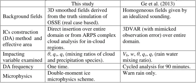
Table 2.1 is provided as a concise summary of the cloud analysis procedure described above.

Table 2.1 Summary ARPS complex cloud analysis procedure

Step Content State variables changed 1 State variables initialization

Model state variables (p, θ, qv, w, qx) read from

background files.

None. 2 Cloud coverage

analysis

Cloud coverage and cloud distribution variables (cloud base and cloud top) analyzed based on Zobs.

None.

3

Cloud associated variables

analysis

1) Cloud mass variables analyzed based on pbg, θbg,

and other cloud info (from step 2).

2) In-cloud vertical velocity (wcld) analyzed based on

cloud type and thickness.

qc, qi.

4 Cloud mass limit 1#

Cloud mass variables adjusted to confine to background qv*.

qc, qi.

5 Precipitation mass analysis#

Precipitation mass variables analyzed based on Zobs

using radar simulator formulation selected.

qr, qs, qh.

6 Cloud mass limit ₂ Cloud mass limited to 5% of precipitation mass in _{avoiding double counting.} qc, qi. 7

In-cloud temperature adjustment#

Temperature adjusted in selected physical manner (LH or MA). θ. 8 In-cloud moisture adjustment#

1) Moisture saturated for grid with observed echo. 2) qv limited to 0.5qv* for grids with analyzed total

mass less than background total mass.

qv.

9

In-cloud vertical motion

adjustment#

(37)

2.2.2 A Modified Mixing Ratio Analysis Procedure

As introduced in the previous section, the mixing ratio analysis procedure available in the current ARPS complex cloud analysis package is relatively simple. In other words, the physics involved are not sufficient in depicting realistic mechanisms and therefore may provide unbalanced analysis results that are incompatible with the complicated model microphysics schemes. As a result, the effect of analysis will not be able to last long as the model goes through a rapid adjustment.

Our study has developed a more general procedure to derive an analysis of the mixing ratios. This procedure is based on the radar operator built by Jung et al. (2008; referred to as JZX hereafter). Four major features that distinguish our approach from the currently utilized procedure are described below:

(i) Unlike the empirical fitting relationships used for developing the KRY operators, the JZX formulation includes the theory of electromagnetic wave propagation and scattering. Factors that affect the scattering results are considered in the derivation; for instance, the dielectric factor and canting behavior as the particle falls. Since the Rayleigh approximation is applied while formulating for the large sized particles such as hailstones, this procedure is currently good for assimilating radar data at long wavelengths (i.e., S band) only.

(ii) Compared to the simple exponential relation between reflectivity and hydrometeor mixing used in KRY, the drop size distribution (DSD) parameters corresponding to the hydrometeors are also included in expressing the radar variables, making this procedure more flexible and therefore compatible with the model using multi-moment (MM) microphysics schemes.

(38)

(iii) Although the melting process of snow is included in the Ferrier operators, this classifying criterion is purely based on temperature with an arbitrary threshold of 0 °C. As much more complicated microphysics and various hydrometeor phases can be expected for their existence in the real atmosphere, a melting ice model is included in JZX to account for sufficient variety of physical properties associated with the melting process (e.g., density change). With this model, the radar variables are not only contributed by the pure precipitating species (e.g., rain, snow, hail), but also by the mixing species (or mixtures, e.g., wet snow, wet hail) if present.

(iv) Considering that different combinations of precipitating species can be used in different NWP models and microphysics schemes, an equation set for graupel species is added to the original published JZX operators, which included only rain, snow, and hail. This addition allows the cloud analysis procedure to handle situations where both hail and graupel species are present.

As mentioned in the previous section, perquisite information about the distribution of multiple hydrometeor species is required before we can retrieve the corresponding mixing ratios based on the Z operators. In the current cloud analysis package, a simple strategy is used to classify for the hydrometeor type based on observed Z and background T when no hydrometeor field is available in the background:

If ≥ 50 dBZ → pure hail is classified,

If < 50 dBZ, and , If -. ≥ 1.3℃ → Pure rain is classified

If -. < 1.3℃ → Pure snow is classified ,

in which Twb is the wet bulb temperature. After the hydrometeor type is determined,

corresponding equations of Z operators is used to compute for the mixing ratio. With this strategy, only one type of hydrometeor can be found for each analyzed grid, which

(39)

is believed unrealistic compared to what is observed in the real atmosphere. Since one major advantage of our modified mixing ratio analysis procedure is the allowance of microphysical complexity (by implementation of the melting model), it is designed to enable the analysis result of a more flexible hydrometeor distribution. To realize our analysis with this modified procedure, the ratio among qx of each pure precipitation

species (i.e., rain, snow, graupel, and hail) is required in advance. As long as there is hydrometeor information available in the background field (usually from previous model forecasts), a more realistic hydrometeor analysis and accompanying microphysical features can be anticipated with our modified procedure.

Details about the formulation with associated parameters and coefficients, and how to perform this modified procedure for mixing ratio analysis in practice can be referred to Appendix A. Although there are observation operators built for other polarimetric variables (e.g., ZDR, KDP) in Jung et al. (2008a), only the reflectivity

operators are adopted in this study to analyze the mixing ratios for its robustness of behavior to various hydrometeors, which also provides us confidence in the analysis results. Operators of other polarimetric variables could also be used; however, comprehensive understanding about the sensitivity of these variables to different hydrometeors and a thorough data quality control process are highly recommended before actual application.

2.3 The Use of Polarimetric Radar Measurements in the Cloud Analysis 2.3.1 Mixing Ratio Analysis Using Polarimetric Radar Variables

Given the additional measurements that polarimetric radar can provide, its advantage over the traditional Doppler radar in better characterizing the hydrometeor

(40)

features and their corresponding microphysical processes has been widely discussed and demonstrated in numerous present studies, particularly in the field of quantitative precipitation estimation (QPE; Bringi and Chandrasekar 2001; Vivekanandan et al. 1999; Zhang et al. 2001; Zrnic and Ryzhkov 1996). Toward the goal of improved short-range forecasts of cloud, hydrometeor, and precipitation, a modified mixing ratio analysis procedure that makes use of multiple polarimetric radar variables is proposed.

The JZX reflectivity operator as described in previous section is used to carry out the procedure. The major role of the extra polarimetric variables, in addition to Z, is to partition the portions of multiple precipitation species required as the prerequisite for the mixing ratio analysis. A fuzzy-logic based hydrometeor classification algorithm (HCA) proposed by Park et al. (2009) is adopted. Variables used for the HCA procedure includes Z, ZDR, KDP, and ρhv. These measurements are firstly interpolated to the model

gridded coordinate. For grids where all four variables are available, the aggregation value Ai for each possible defined class of radar echo is computed as

3 =∑96:;_∑567 8₅ 6

6 9

6:; ,

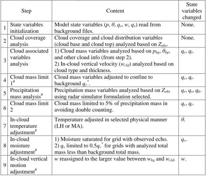
where i represents the ith class of echo that could be classified by the algorithm, j represents the jth of radar variables, P(i)(Vj) is a trapezoidal shape membership function

that characterizes the distribution of the jth variable for the ith class (shown as FIG. 2.1), and Wij is a discriminating efficiency based weight between 0 and 1 assigned to the ith

class and the jth variable. As a result, Ai values ranging from 0 to 1 for ten classes: 1)

ground clutter (GC); 2) biological scatterers (BS); 3) dry aggregated snow (DS); 4) wet snow (WS); 5) ice crystals (CR); 6) graupel (GR); 7) big drops (BD); 8) light to

(41)

For specific values of Wij or the X1, X2, X3, and X4 in P(i)(Vj), please refer to Park et al.

(2009).

FIG. 2.1 Trapezoidal membership function, where X is an arbitrary radar variable. Adapted from Park et al. (2009).

In our adoption described above, couple simplifications upon the (Park et al. 2009)’s original proposal have been taken in calculating the aggregation values. First, two texture parameters SD(Z) and SD(ФDP) (along radial fluctuation of Z and ФDP,

respectively) are excluded. As these two variables are mainly included to identify the non-meteorological echo, the impact of this omission on the classification results can be minimized by pre-processing radar data with some quality control (QC) algorithms (Hubbert et al. 2009). Second, the Qj, confidence vector, present in both numerator and

denominator of the original Ai equation is also omitted. As the Qj is designed to account

for the measurement error of each variable used, even confidence on each variable is accordingly implied while this simplification is taken.

After the Ai values are obtained, the results are further examined by some

empirical hard thresholds (Table 2.2) to suppress apparently unrealistic class designations. For example, the radial velocity V interpolated on model grids is used to

(42)

eliminate the likelihood of the occurrence of ground clutter: when V is greater than 1.0 m s-1, A1 (1 is the order number for GC class) is directly set to 0. The rules are based on

both physical model and observations (Straka et al. 2000).

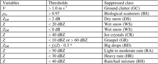
Table 2.2 Empirical hard thresholds used to suppress apparently wrong designations (reproduced from Park et al. 2009)

Variables Thresholds Suppressed class

V > 1.0 m s-1 Ground clutter (GC) ρhv > 0.97 Biological scatterers (BS) ZDR > 2 dB Dry snow (DS) Z < 20 dBZ Wet snow (WS) ZDR < 0 dB Wet snow (WS) Z > 40 dBZ Ice crystals (CR) Z < 10 dBZ or > 60 dBZ Graupel (GR) ZDR < f2(Z) - 0.3 * Big drops (BD)

Z > 50 dBZ Light to moderate rain (RA)

Z < 30 dBZ Heavy rain (HR)

Z < 40 dBZ Rain/hail mixture (RH)

*f2(Z) is a function of Z (in dBZ) that can be found in Park et al. (2009).

It has been indicated that additional routines that account for factors such as relative location of radar sampling volume with respect to the melting layer (ML) and precipitation nature (i.e., convective versus stratiform) are required for better classification results (Heinselman and Ryzhkov 2006). In our procedure, the background temperature is used for locating the ML top (where T begins to drop below 0 °C) and a constant depth of 500 m below the ML top is used for defining the layer. Any non-meteorological class (GC or BS), WS, and RA are excluded above the ML top regions, where strict frozen condition is presumed. On the other hand, the intensity of observed Z profile is used to classify the precipitation type. The following simple empirical strategy is used:

(43)

For grids below ML bottom, B if ≥ 35 CD → Convective._{if < 35 CD → Stratiform.} For grids within ML, B if ≥ 35 CD HIC Lower successive grid is Conv. → Convective. _{otherwise → Stratiform.} For grids above ML top, B if ≥ 30 CD → Convective._{if < 30 CD → Stratiform.} The condition to check the lower successive grid is applied to prevent potential contamination of bright band, which is known for great Z intensity. Snow classes (i.e., DS and WS) are excluded for convective precipitation while the convective hydrometeor types such like BD, GR, and RH are avoided in stratiform area.

After all despeckling processes described above are gone through and all physical unreasonable classes are avoided, the survivals of Ai are used for determining

relative portion of different precipitation hydrometeors. All eight meteorological classes are classified into three types as:

1) Rain type: BD, RA, and HR. 2) Snow type: DS, WS, and CR. 3) Hail/Graupel type: GR and RH.

The Ai maximum of each type is taken for representing the portion of that specific type.

Specifically, the ratio among rain, snow, and hail/graupel is determined as: max(A7 , A8 , A9) : max(A3 , A4 , A5) : max(A6 , A10).

The mixing ratio of each type is then analyzed using the JZX reflectivity operator to comply with the Z observation. Refer to Appendix A for detailed mathematical formulation.

The principal assumption incorporated in this procedure is that the aggregation values calculated from HCA are quantitatively proportional to the hydrometeor content (i.e., mixing ratio). One main feature of the analysis result from this HCA-based

(44)

procedure is that coexistence of different hydrometeors is possible at a same location, which is believed more realistic. Demonstrations of the analysis result will be shown and discussed in the coming sections with a real case application.

2.3.2 A Mei-Yu Front Mesoscale Convective Vortex and Model Configuration

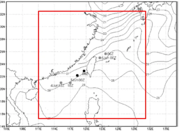
During the intensive observing period (IOP) 6 (1800 UTC 4 June to 1200 UTC 6 June) of the Southwest Monsoon Experiment (SoWMEX) and the Terrain-influenced Monsoon Rainfall Experiment (TiMREX), a joint Taiwan-United States field experiment (Jou et al. 2010) taking place in 2008 Mei-Yu season (Chen and Chang 1980), a MCV embedded in a quasi-stationary mei-yu front across the southern China and middle Taiwan was observed. As the MCV-associated convective system moved in, serious flood was resulted in the southwestern coastal area of Taiwan with nearly 200 mm precipitation in two hours (Lai et al. 2011). FIG. 2.2 shows the track of the MCV.

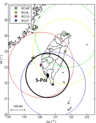
In addition to the four S-band Doppler radars operated by the Central Weather Bureau (CWB), the National Center for Atmospheric Research’s (NCAR’s) S-band polarimetric Doppler research radar (as S-Pol hereafter) was deployed at southwest coast of Taiwan for the SoWMEX/TiMREX project. The radars locations are provided in FIG. 2.3.

The ARPS model and its data assimilation system are used to examine the impact of the mixing ratio analysis procedure based on polarimetric variables (as described in previous section) on the very short-range (1 hour) precipitation forecast. The domain, as marked by the red square in FIG. 2.2, is designed to cover the Southeast Asia with Taiwan in the center of the domain (121 °E, 24 °N). Although the MCV of interest was located very close to Taiwan in our study period, our domain is created as

(45)

large as this to avoid any potential over-stressed forcing from the lateral boundary conditions (LBCs). A northern hemisphere Lambert Conformal map projection is used. The domain has 803 (x-direction) × 803 (y-direction) × 53 (z-direction) grid points in total with 2.5 km horizontal spacing and an averaged 420 m vertical resolution. Terrain-following and stretching vertical coordinate is used with the lowest level of 50 m AGL.

FIG. 2.2 Weekly averaged sea surface temperature during 2-8 June 2008 and MCV track. Gray dots and black dots are tracked by IR satellite images and radar radial velocity, respectively. Red square denotes the domain of our simulation. Reproduced from Lai et al. (2011).

(46)

FIG. 2.3 Distribution of four CWB operational radars and NCAR S-Pol radar. Observing ranges are denoted by circles in corresponding colors (200 km for CWB radars and 150 km for NCAR S-Pol).

The simulation is initialized at 00 Z 5 June 2008 utilizing the CWB operational WRF analysis after interpolating from the original in 15-km grid spacing to our 2.5-km grids. The radial velocities (Vr) observed by S-Pol are assimilated using the ARPS

3DVAR package. Two sets of experiment are performed with different mixing ratio analysis procedures: one with current available procedure (based on Z only) using KRY operator, and the other with the HCA procedure (based on Z and other polarimetric variables) using JZX operator. Under each experiment, two microphysics parameterization schemes: Lin single-moment (Lin et al. 1983) and MY double-moment (Milbrandt and Yau 2005a, 2005b) are implemented; a total of four