Deep learning based pipeline for fingerprinting using brain functional MRI connectivity data

(1)

ScienceDirect

Available online at www.sciencedirect.com

Procedia Computer Science 141 (2018) 539–544

This is an open access article under the CC BY-NC-ND license (https://creativecommons.org/licenses/by-nc-nd/4.0/) Selection and peer-review under responsibility of the scientific committee of ICTH 2018.

10.1016/j.procs.2018.10.129

This is an open access article under the CC BY-NC-ND license (https://creativecommons.org/licenses/by-nc-nd/4.0/)

Selection and peer-review under responsibility of the scientific committee of ICTH 2018.

1877-0509

ScienceDirect

www.elsevier.com/locate/procedia

This is an open access article under the CC BY-NC-ND license (http://creativecommons.org/licenses/by-nc-nd/3.0/). Selection and peer-review under responsibility of the scientific committee of ICTH 2018

The 2nd International Workshop on Healthcare Interoperability and Pervasive Intelligent Systems (HiPIS 2018)

Deep Learning Based Pipeline for Fingerprinting Using Brain

Functional MRI Connectivity Data

Nicolás F. Lori

a,b,c,

_{*, Ivo Ramalhosa}

c

_{, Paulo Marques}

a,b

_{, Victor Alves}

c

a_{Life and Health Sciences Research Institute (ICVS), School of Medicine, University of Minho, 4710–057 Braga, Portugal} b_{ICVS/3B’s – PT Government Associate Laboratory, 4710–057 Braga, Portugal}

c_{Centre Algoritmi, University Of Minho, 4710–057 Braga, Portugal}

Abstract

In this work we describe an appropriate pipeline for using deep-learning as a form of improving the brain functional connectivity-based fingerprinting process which is connectivity-based in functional Magnetic Resonance Imaging (fMRI) data-processing results. This pipeline approach is mostly intended for neuroscientists, biomedical engineers, and physicists that are looking for an easy form of using fMRI-based Deep-Learning in identifying people, drastic brain alterations in those same people, and/or pathologic consequences to people’s brains. Computer scientists and engineers can also gain by noticing the data-processing improvements obtained by using the here-proposed pipeline. With our best approach, we obtained an average accuracy of 0.3132 ± 0.0129 and an average validation cost of 3.1422 ± 0.0668, which clearly outperformed the published Pearson correlation approach performance with a 50 Nodes parcellation which had an accuracy of 0.237.

This is an open access article under the CC BY-NC-ND license (http://creativecommons.org/licenses/by-nc-nd/3.0/).

Keywords: Deep-Learning; fMRI Fingerprinting; Data-processing Pipeline; 1. Introduction

Neuroimaging has a major clinical application as medical support in neurology, more properly in the diagnosis and integrative medicines [1][2]. In neuroimaging, the study of brain structure is not enough, since it doesn’t give relevant information for the diagnosis of pathologies where structural alterations are not anatomically detected. Therefore, a

* Corresponding author. Tel.: +351 253 604 800; fax: +351 253 604 809. E-mail address: [email protected]

ScienceDirect

www.elsevier.com/locate/procedia

This is an open access article under the CC BY-NC-ND license (http://creativecommons.org/licenses/by-nc-nd/3.0/). Selection and peer-review under responsibility of the scientific committee of ICTH 2018

The 2nd International Workshop on Healthcare Interoperability and Pervasive Intelligent Systems (HiPIS 2018)

Deep Learning Based Pipeline for Fingerprinting Using Brain

Functional MRI Connectivity Data

Nicolás F. Lori

a,b,c,

_{*, Ivo Ramalhosa}

c

_{, Paulo Marques}

a,b

_{, Victor Alves}

c

a_{Life and Health Sciences Research Institute (ICVS), School of Medicine, University of Minho, 4710–057 Braga, Portugal} b_{ICVS/3B’s – PT Government Associate Laboratory, 4710–057 Braga, Portugal}

c_{Centre Algoritmi, University Of Minho, 4710–057 Braga, Portugal}

Abstract

In this work we describe an appropriate pipeline for using deep-learning as a form of improving the brain functional connectivity-based fingerprinting process which is connectivity-based in functional Magnetic Resonance Imaging (fMRI) data-processing results. This pipeline approach is mostly intended for neuroscientists, biomedical engineers, and physicists that are looking for an easy form of using fMRI-based Deep-Learning in identifying people, drastic brain alterations in those same people, and/or pathologic consequences to people’s brains. Computer scientists and engineers can also gain by noticing the data-processing improvements obtained by using the here-proposed pipeline. With our best approach, we obtained an average accuracy of 0.3132 ± 0.0129 and an average validation cost of 3.1422 ± 0.0668, which clearly outperformed the published Pearson correlation approach performance with a 50 Nodes parcellation which had an accuracy of 0.237.

This is an open access article under the CC BY-NC-ND license (http://creativecommons.org/licenses/by-nc-nd/3.0/).

Keywords: Deep-Learning; fMRI Fingerprinting; Data-processing Pipeline; 1.Introduction

Neuroimaging has a major clinical application as medical support in neurology, more properly in the diagnosis and integrative medicines [1][2]. In neuroimaging, the study of brain structure is not enough, since it doesn’t give relevant information for the diagnosis of pathologies where structural alterations are not anatomically detected. Therefore, a

* Corresponding author. Tel.: +351 253 604 800; fax: +351 253 604 809. E-mail address: [email protected]

(2)

method to assess brain function is necessary. This led to the development of functional Magnetic Resonance Imaging (fMRI), which is a technique that monitors hemodynamic events related to changes in neuronal activation in the brain by relying on the Blood Oxygenation Level Dependent (BOLD) contrast [3][4], including functional integration [5]. Functional Connectivity (FC) is based on the temporal correlation between spatially remote neurophysiological events in the brain [6][7]. The FC can be based in different types of fMRI data, but usually the data-type used is resting-state BOLD fMRI (rs-fMRI) [8] in which case the FC provides information about the default brain connectivity.

There are three main methods used by the neuroimaging community to analyze and evaluate FC: Seed-Based Analysis (SBA), Independent Component Analysis (ICA) and connectomic analysis which is the method we will use in this work. The connectomic analysis obtains the interactions between every possible pair of brain regions. The connectomic data is typically represented as a connectivity matrix. The connectivity matrix is the schematization in matrix form of the values of the correlation between all pairs of regions. So, its size is N x N, where N is the number of regions or nodes resulting from the brain parcellation, and it has been used to study changes in the (brain functionality) due to a particular disease, such as Alzheimer’s Disease (AD) [9] or autism [10]; and also study physiological trait [11]. These matrices are used for classification (e.g. by recurring to Machine Learning (ML)).

In recent work [12], those FC matrices have been able to discriminate preterm infants at term-equivalent age and healthy/normal-born controls with 80% accuracy using a ML method. Plus, their approach was used to distinguish between healthy controls and depressed patients with accuracy values of 85.85% and 70.75%, respectively for patients with treatment resistant depression and patients with non-treatment resistant depression [13]. Furthermore, these connectivity matrices have shown to be reliable fingerprints, making possible to identify accurately a specific subject from a large group. The research made in Functional Connectome Fingerprinting which identified individuals using FC patterns [14] demonstrated that when applied to rs-fMRI data, these methods can predict and identify an individual, respectively, with 92.5% and 94.4% accuracy. For fMRI acquisition in task conditions, they also got results that presented a great accuracy, with rates of about 87.3%.

The work developed here aims at improving over results obtained in previous work [14], wherein the functional connectivity provided from rs-fMRI data is used as the subjects’ fingerprint. Hence, the approach followed in this work will be compared with the approach presented in ref. [14]. The approach of ref. [14] used two different sessions of rs-fMRI acquisition, obtained in different days, as the subjects’ set. Plus, each correlation matrix with FC data for each session was correlated by Pearson’s correlation with all the other FC matrices in the other session.

The approach to FC in this work is based on ML techniques. So, there is always a learning-process to obtain both an accurate representation of data and prior knowledge [15]. The major novelty in our approach is the use of Deep Neuronal Networks (DNN), which uses Artificial Neural Networks (ANN) for modelling, to these standard rs-fMRI-based FC data, to achieve a better classification [16]. The FC values allow the features’ granularity to be diversified, where the unit in study can be a voxel, or a parcellated brain-region [17][18].

2.Materials

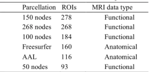
The different atlases have different number of ROIs, and different creation processes by use of different MRI data types (Table 1). The number of nodes doesn’t coincide [19] with the total number of anatomical regions of the used atlas, such as the AAL atlas [20] or the Freesurfer atlas [21], because the name is associated to the number of “seeds” used in each cerebral hemisphere during the atlas application process.

The rs-fMRI data used in this work was obtained from the

SWITCHBOX project realized at ICVS (see Acknowledgments and filiations), named here as: “ICVS data” [23]. We chose to use this ICVS data set as it was obtained from a 1.5 T MR clinical scanner similar to the scanners more commonly used worldwide [24].

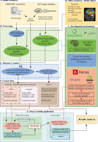
The data used in this work are volumes with the temporal data saved from rs-fMRI. Initially, the data is a set of DICOM brain images of different temporal points of the fMRI data-acquisition which are converted into a single 4D volume file (Fig. 1D).

Table 1. Atlases versus number of ROIs descending order.

Parcellation ROIs MRI data type 150 nodes 278 Functional 268 nodes 268 Functional 100 nodes 184 Functional Freesurfer 160 Anatomical AAL 116 Anatomical 50 nodes 93 Functional

(3)

These fMRI data-set labels are the identity information of the subject (e.g. gender, state in a disease, blood type). These labels are information that will be used in the supervised learning for training, validation and testing of the DL models. Before the DL-pipeline, the fMRI data undergoes an FC-pipeline to obtain a FC file with the values of the correlation of fMRI intensities between each of brain region pair, for each of the 76 subjects (39 male and 37 female) (Fig. 1E). The scanner used was a Siemens 1.5 T MRI scanner with a 12-channel receive-only head-coil. The rs-fMRI was obtained using BOLD sensitive Echo-Planar Imaging (EPI) sequence with these parameters: 30 axial slices; TR/TE = 2000 ms/30 ms; flip angle = 90º; slice thickness = 3.5 mm; slice gap = 0.48 mm; voxel size = 3.5 x 3 x 3.5 mm2_{; FoV = 1.344 mm. Before the FC-pipeline, there is a standard FSL data-processing of the rs-fMRI data which}

obtains a file with 355 lines, one for each of the volumes of the acquisition with the mean BOLD signal for each region of the brain datasets. After the FC-pipeline, there are two types of data: the FC, and the respective subject’s labels (Fig. 1F).

The FC data was analyzed by use of the correlation matrix (a.k.a. ROIs FC analysis method). Each FC input file has one line for each volume in the acquisition, and one column for each region of the atlas used in the parcellation process (e.g. the average value for each volume and region). The static FC was computed through the Pearson’s correlation between the full time-series of each pair of brain regions, resulting in the symmetric matrix with the Pearson’s coefficients expressed in one adjacency matrix per subject [7][25]. Then a Fisher’s r-to-Z transformation was applied to each correlation matrix to improve the normality of the correlation coefficients.

3.Methods

The DL module (Fig. 1G) obtains the best models and their respective results. Thus, the use of the DL module enabled a better automation of processes, an easier and more efficient data management, and the creation of a workflow which deals with the FC information and uses it as the features for the construction of DL models allowing an improvement in subject’s classification. This DL processing is a reliable method for applications in FC obtained from rs-fMRI data, in which we used a recent library Nipy [26] based in the Python programming language [27] (Fig. 1C) with several advantages for the workflow. The datasets creation, which includes the analysis of the values by dataset and subject, or by class of the dataset, is then prepared for use in the training, validation and test of DL models (Fig. 1C). Finally, the major objective, the DL application over the FC data to improve the subject’s classification tasks includes the

fine-tuning of the models, the selection of the best models, and the analysis and management of the different results (Fig. 1G).

(4)

The development environment used in this work is represented in Figure 2. All development work was based in the Python programming language [27]. To download and manage the different packages used in this work we used anaconda [28]. Plus, to support the different parts of the work we used PyDev, a Python Integrated Development

Environment (IDE), for Eclipse. Most of the work was developed and tested by using either the bash console or the interactive console of Python (iPython). Finally, to increase computation velocity this work used the Compute Unified Device Architecture (CUDA), a parallel computing platform and programming model developed by NVIDIA [29] which uses graphical processing units (GPUs) in different computation tasks (Fig. 1C and Fig. 2). The use of CUDA permits the use of GPUs as the computation unit of the DL application. All the software ran on servers with Ubuntu operating system.

We tested two different DL models, each of them based in one of two different types of layers: fully connected layers, and convolutional layers. For each of the two types of layers, we then tested architectures with different depths. The plan was thus to design a small DL framework (see Fig. 1G) working alongside other methods, as part of a bigger framework, where this small framework could deal with the FC matrices extracted from the rs-fMRI data. The small DL framework was divided in two major parts: the fine-tuning models, and the final models (Fig. 1G). The fine-tuning part is responsible for the continuous adjustment of the model so that the model passes on to the final phase. In the final phase, the deeper tests are done, with increasing number of repetitions, and where the model and the model’s performance values are saved for future uses. The validation of each model is made manually, after analysis of the performance measurements.

4.Results and Discussion

In ref. [14], the process applied to compare the FC matrices was the similarity-based Pearson’s correlation where for each subject it is made a Pearson’s correlation between that subject’s FC matrix obtained in an experimental session (the target matrix), and the other existent FC matrices obtained in different experimental sessions (the database matrices). Then, it is only chosen the database FC matrix with the maximum correlation value (the chosen matrix). If the chosen matrix and the target matrix are of the same subject, then the classification is correct, and so the classification score obtained is 1. If it is not the same subject, then the classification is incorrect, and the obtained classification score is 0. To test the approach, we applied the procedure of ref. [14] to the 1.5T MRI ICVS data, and obtained static FC for the set of atlases used in this work, and the obtained results are presented in Table 2. These values in Table 2 are the objective

values to be outperformed by the DL approach developed here.

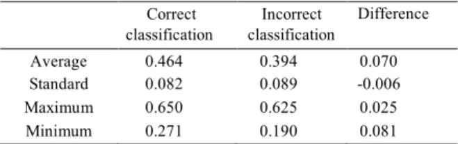
By analyzing the average

correlations values for correct and incorrect classifications, it was verified that the correlation value affects positively the classification result. And again, the difference between the two situations was significant. Therefore, the amount of correlation value also is

correlated with the average accuracy over the dataset (see Table 3).

The principal additions to the initial simple fully connected layer model towards more complex systems were the increase depth and the adding of convolutional networks. Doing the fine-tuning of the learning process for each parcellation and session prediction would require an exceedingly long time. As our dataset has 76 subjects, the probability of correct classification by a random process is 1/76»0.01316. The selection process of the best set of hyperparameters begins by using the 50 nodes atlas, for it has the fewer number of features and it has the worst results. Hence, it will have a greater interval for improvement with a lesser number of parameters, and thus less features to

Fig. 2. Development environment schema with the support technology

Table 2. Different parcellation obtained values using approach of ref. [14] for our data

Predict session 1 Predict session 2

Parcellation Value Diff. Parcellation Value Diff. 150 nodes 0.342 0.000 150 nodes 0.342 0.0000

100 nodes 0.316 0.026 268 nodes 0.303 0.0395 268 nodes 0.316 0.026 100 nodes 0.289 0.0526 Freesurfer 0.263 0.079 AAL 0.276 0.0658 AAL 0.250 0.092 Freesurfer 0.250 0.0921

(5)

learn. The first set of hyperparameters wasn’t selected randomly but by use of several references [12][14][22][30], and also some experiments were made before testing the models. The models used amount to a total of 135 different models, and for each model we make 10 tests, with each test having a different set of alpha rates used for the activation function Leaky ReLU.

The results demonstrated that the best alpha is 0.8, which implies that to obtain better classifications results, the models give some importance (near 1) to the negatives values in the dataset. It is relevant to emphasize that in these tests, we only intend to get a comparison between the results for different tests, and not already aim for the best model.

The probability of the improvement with the increase of epochs is very likely, as the training accuracy continually

increases as the epochs increase, and so does the learning process. As mentioned before, the number of combinations in analysis are 135, wherein 15 models with different loss and activation function were tested for 9 learning rates. After analyzing the 15 different models for different parameters, it was obtained that the best model for a 50 Nodes parcellation, for both accuracy and cost, was the model with the parameters described in Table 4. This best model obtained an average accuracy of 0.3132 ± 0.0129 and an average validation cost of 3.1422 ± 0.0668, which clearly outperformed the published Pearson correlation approach performance with a 50 Nodes parcellation [14], which had a validation accuracy of 0.237.

5.Conclusion

To compare the different models, we used a set of metrics to assess the performance of the model and to compare it with other models and hence fine-tune the different hyperparameters of the model. Some metrics were used to assess the behavior of the model in both training and validation, such as, accuracy and loss. In addition to the final values, other values are calculated during the training, such as maximum accuracy in validation with the

corresponding epoch occurrence, the differences between the different data (e.g. training and validation), and others. The different metrics used were always saved.

The cross-validation was not possible to use since for the static FC there were too few cases for each label. Thus, the best approach was to divide the FC data of each acquisition session into two equal parts, one part being used as the validation data and the other is used as the test data.

The approach proposed here comprehends the pre-processing of the raw data, the creation of datasets with different functional connectivity information, and the creation of a DL module which helps fine-tune the different DL models before getting the best model, which is then used to make the final analysis.

Acknowledgements

Thanks to Eduarda Sousa for support. NFL was supported by a fellowship of the project MEDPERSYST - POCI-01-0145-FEDER-016428, funded by Portugal’s FCT. This work was also supported by NORTE-01-0145-FEDER-000013, and NORTE 2020 under the Portugal 2020 Partnership Agreement through the FEDER, plus it was funded by the European Commission (FP7) “SwitchBox - Maintaining health in old age through homeostasis” (Contract HEALTH-F2-2010-259772), and co-financed by the Portuguese North Regional Operational Program (ON.2 – O Novo Norte), under the QREN through FEDER, and by the “Fundação Calouste Gulbenkian” (Portugal) (Contract grant number: P-139977; project “TEMPO - Better mental health during ageing based on temporal prediction of individual brain ageing trajectories”). We gratefully acknowledge the support of the NVIDIA Corporation with their donation of a Quadro P6000 board used in this research. This work was also supported by COMPETE: POCI-01-0145-FEDER-007043 and FCT within the Project Scope: UID/CEC/00319/2013.

Table 3. Correlations values in the correct and incorrect classifications, and respective difference for our data.

Correct

classification classification Incorrect Difference Average

value 0.464 0.394 0.070

Standard

Deviation Maximum 0.082 0.650 0.089 0.625 -0.006 0.025

Minimum 0.271 0.190 0.081

Table 4. Best Model Parameters (Batch size=# Hidden Layers=1), with Adjustable Learning-Rate [Init.=0.001, Best =0.0001]

Parameter Value Activation functions Tanh

Loss Function Categorical cross-entropy

Optimizer RMSprop

Kernel Initializer Glorot Uniform

Bias Initializer Random Uniform

Nodes per hidden layer 200 fMRI Data Temporal

Filtering

(6)

References

[1] Lane R D, Wager, T D. 2009. Introduction to a Special Issue of Neuroimage on Brain-Body Medicine. NeuroImage, 47(3), 781–784. https://doi.org/10.1016/j.neuroimage.2009.06.004

[2] Horwitz B, Smith J F, Jacobs J, Kahana M J, Aimone J B, Wiles J, … Lim W A. 2009. What’s new in neuroimaging methods? Annals of the New York Academy of Sciences, 14(4), 260–293. https://doi.org/10.1111/j.1749-6632.2009.04420.x.What

[3] Functional Magnetic Resonance Imaging (fMRI). 2009. In Encyclopedia of Neuroscience (pp. 1652–1652). Berlin, Heidelberg: Springer Berlin Heidelberg. https://doi.org/10.1007/978-3-540-29678-2_1873

[4] Ogawa S, Lee T M, Kay A R, Tank D W. 1990. Brain magnetic resonance imaging with contrast dependent on blood oxygenation. Proceedings of the National Academy of Sciences of the United States of America, 87(24), 9868–72. https://doi.org/10.1073/pnas.87.24.9868

[5] Smith S M. 2012. NeuroImage The future of FMRI connectivity. NeuroImage, 62(2), 1257–1266. https://doi.org/10.1016/j.neuroimage.2012.01.022

[6] Friston K J. 1994. Functional and effective connectivity in neuroimaging: A synthesis. Human Brain Mapping, 2(1–2), 56–78. https://doi.org/10.1002/hbm.460020107

[7] Biswal B, Yetkin F Z, Haughton V M, Hyde J S. 1995. Functional connectivity in the motor cortex of resting human brain using echo-planar MRI. Magnetic Resonance in Medicine, 34(4), 537–41. Retrieved from http://www.ncbi.nlm.nih.gov/pubmed/8524021

[8. Gusnard D A, Raichle M E. 2001. Searching for a baseline: functional imaging and the resting human brain. Nature Reviews. Neuroscience, 2(10), 685–94. https://doi.org/10.1038/35094500

[9] Dennis E L, Thompson P M. 2014. Functional brain connectivity using fMRI in aging and Alzheimer’s disease. Neuropsychology Review, 24(1), 49–62. https://doi.org/10.1007/s11065-014-9249-6

[10] Maximo J O, Cadena E J, Kana R K. (2014o). The implications of brain connectivity in the neuropsychology of autism. Neuropsychology Review, 24(1), 16–31. https://doi.org/10.1007/s11065-014-9250-0

[11] Jung W H, Prehn K, Fang Z, Korczykowski M, Kable J W, Rao H, Robertson D C. 2016. Moral competence and brain connectivity: A resting-state fMRI study. NeuroImage, 141, 408–415. https://doi.org/10.1016/j.neuroimage.2016.07.045

[12] Ball G, Aljabar P, Arichi T, Tusor N, Cox D, Merchant N, …, Counsell S J. 2016. Machine-learning to characterise neonatal functional connectivity in the preterm brain. NeuroImage, 124, 267–275. https://doi.org/10.1016/j.neuroimage.2015.08.055

[13] Byun H Y, Lu J J, Mayberg H S, Günay C. 2014. Classification of Resting State fMRI Datasets Using Dynamic Network Clusters. Modern Artificial Intelligence for Health Analytics, 14, 2–6.

[14] Finn E S, Shen X, Scheinost D, Rosenberg M D, Huang J, Chun M M, …, Constable R T. 2015. Functional connectome fingerprinting: Identifying individuals using patterns of brain connectivity. Nature Neuroscience, 18(11), 1664–1671. https://doi.org/10.1038/nn.4135 [15] Suzuki K, Yan P, Wang F, Shen D. 2012. Machine learning in medical imaging. International Journal of Biomedical Imaging, 2012, 2012–

2014. https://doi.org/10.1155/2012/123727

[16] LeCun Y, Bengio Y, Hinton G. 2015. Deep learning. Nature, 521(7553), 436–444. https://doi.org/10.1038/nature14539

[17] Wang P, Ge R, Xiao X, Cai Y, Wang G, Zhou F. (2016c). Rectified-Linear-Unit-Based Deep Learning for Biomedical Multi-label Data. Interdisciplinary Sciences: Computational Life Sciences. https://doi.org/10.1007/s12539-016-0196-1

[18] Greenspan H, Van Ginneken B, Summers R M. 2016. Guest Editorial Deep Learning in Medical Imaging : Overview and Future Promise of an Exciting New Technique. IEEE Transactions on Medical Imaging, 35(5), 1153–1159. https://doi.org/10.1109/TMI.2016.2553401 [19] Shen, X., Tokoglu, F., Papademetris, X., & Constable, R. T. (2013ax). Groupwise whole-brain parcellation from resting-state fMRI data for

network node identification. NeuroImage, 82, 403–415. https://doi.org/10.1016/j.neuroimage.2013.05.081

[20] Tzourio-Mazoyer N, Landeau B, Papathanassiou D, Crivello F, Etard, O, Delcroix N, …, Joliot M. 2002. Automated Anatomical Labeling of Activations in SPM Using a Macroscopic Anatomical Parcellation of the MNI MRI Single-Subject Brain. NeuroImage, 15(1), 273–289. https://doi.org/10.1006/nimg.2001.0978

[21] Desikan, R. S., Ségonne, F., Fischl, B., Quinn, B. T., Dickerson, B. C., Blacker, D., … Killiany, R. J. (2006ez). An automated labeling system for subdividing the human cerebral cortex on MRI scans into gyral based regions of interest. https://doi.org/10.1016/j.neuroimage.2006.01.021 [22] Fischl B, Van Der Kouwe A, Destrieux C, Halgren E, Ségonne F, Salat D H, …, Dale A M. 2004. Automatically Parcellating the Human

Cerebral Cortex. Cerebral Cortex, 14(1), 11–22. https://doi.org/10.1093/cercor/bhg087

[23] Magalhães R, Marques P, Soares J, Alves V, Sousa N. 2015. The Impact of Normalization and Segmentation on Resting-State Brain Networks. Brain Connectivity, 5(3), 166–176. https://doi.org/10.1089/brain.2014.0292

[24] Rentz, S. 2012. Your Guide to Medical Imaging Equipment. Block Imaging. in: https://info.blockimaging.com/bid/87030/3t-mri-vs-1-5t-mri]. [25] Al-Rfou R, Alain G, Almahairi A, Angermueller C, Bahdanau D, Ballas N, …, Zhang Y. 2016. Theano: A Python framework for fast

computation of mathematical expressions. Retrieved from https://arxiv.org/pdf/1605.02688.pdf

[26] Gorgolewski, K., Burns, C. D., Madison, C., Clark, D., Halchenko, Y. O., Waskom, M. L., & Ghosh, S. S. (2011ft). Nipype: a flexible, lightweight and extensible neuroimaging data processing framework in python. Frontiers in Neuroinformatics, 5, 13. https://doi.org/10.3389/fninf.2011.00013

[27] Van Rossum G, Drake F L. 2006. Python Reference Manual. October, 22, 9117–9129. https://doi.org/10.1242/jeb.00343

[28] Continuum Analytics. 2016. Anaconda Software Distribution. Retrieved December 6, 2017, from https://docs.anaconda.com/anaconda/faq#how-do-i-cite-anaconda-in-an-academic-paper

[29] NVIDIA Developer. (n.d.-ai). 2017. Retrieved October 12, 2017, from https://developer.nvidia.com/

[30] Byun H Y, Lu J J, Mayberg H S, Günay C. 2014. Classification of Resting State fMRI Datasets Using Dynamic Network Clusters. Modern Artificial Intelligence for Health Analytics, 14, 2–6.