Penalised regression for high-dimensional data: an empirical investigation and improvements via ensemble learning

(1)

Penalised regression for high-dimensional data: an empirical

investigation and improvements via ensemble learning

Fan Wang

Wolfson College

University of Cambridge

This dissertation is submitted for the degree of

Doctor of Philosophy

(2)

Declaration

I declare that the contents presented in this dissertation are the results of my own work except where specified otherwise. I declare that this thesis was composed by myself, and no part of this thesis has been submitted for a degree or other qualification at any university.

The work in Chapter 2together with parts of Chater3have been

sub-mitted for publication. The manuscript is also available as an arXiv

preprint [Wang et al., 2018]. The work in Chapter 4 will shortly be

submitted for publication.

(3)

Acknowledgements

First of all, I would like to thank my supervisors Sylvia Richardson and Steven Hill, for their unwavering support during my PhD studies. Their sharp intuition and deep insights over the past years have been invaluable and have enabled me to finish the thesis much more easily. Their constant patience and encouragement have been of great help, not only for my research, but also for my future career.

I would like to express my appreciation to all the support I received from colleagues and advisers. Particularly, I am deeply grateful to Sach Mukherjee, Gwenael Leday, Paul Kirk and Paul Newcombe for their great advice on improving my work. I wish to thank all members of the MRC Biostatistics Unit for the pleasurable working atmosphere.

My gratitude also goes to all my close friends for their unconditional support in my life. They help me come out of difficult times, and their sharing and listening have meant a lot to me. Particularly, I would like to thank Qiyu Yuan, Alex Yuan, Peicheng Xu, Tien Vo, Jason Xu and Mary Caplinger for always being there for me.

Finally, I would like to thank my family. Without their love and care, I would not have been able to come this far.

(4)

Summary

In a wide range of applications, datasets are generated for which the

number of variables p exceeds the sample size n. Penalised likelihood

methods are widely used to tackle regression problems in these high-dimensional settings. In this thesis, we carry out an extensive empirical comparison of the performance of popular penalised regression meth-ods in high-dimensional settings and propose new methodology that uses ensemble learning to enhance the performance of these methods.

The relative efficacy of different penalised regression methods in finite-sample settings remains incompletely understood. Through a large-scale simulation study, consisting of more than 1,800 data-generating scenarios, we systematically consider the influence of various factors (for example, sample size and sparsity) on method performance. We focus on three related goals — prediction, variable selection and vari-able ranking — and consider six widely used methods. The results are supported by a semi-synthetic data example. Our empirical results complement existing theory and provide a resource to compare perfor-mance across a range of settings and metrics.

We then propose a new ensemble learning approach for improving the performance of penalised regression methods, called STructural RAN-Domised Selection (STRANDS). The approach, that builds and im-proves upon the Random Lasso method, consists of two steps. In both steps, we reduce dimensionality by repeated subsampling of variables. We apply a penalised regression method to each subsampled dataset and average the results. In the first step, subsampling is informed by

(5)

variable correlation structure, and in the second step, by variable im-portance measures from the first step. STRANDS can be used with any sparse penalised regression approach as the “base learner”. In sim-ulations, we show that STRANDS typically improves upon its base learner, and demonstrate that taking account of the correlation struc-ture in the first step can help to improve the efficiency with which the model space may be explored.

We propose another ensemble learning method to improve the predic-tion performance of Ridge Regression in sparse settings. Specifically, we combine Bayesian Ridge Regression with a probabilistic forward selection procedure, where inclusion of a variable at each stage is prob-abilistically determined by a Bayes factor. We compare the prediction performance of the proposed method to penalised regression methods using simulated data.

(6)

Abbreviations

AdaLasso adaptive Lasso

AIC Akaike information criterion

AUC area under the ROC curve

bagging bootstrap aggregation

BF Bayes factor

BIC Bayesian information criterion

Bolasso Bootstrap-enhanced Lasso

ENet elastic net

fMRI functional magnetic resonance imaging

FN false negative

FP false positive

FPR false positive rate

GWAS genome-wide association study

HENet heavy elastic net

LARS least angle regression

Lasso least absolute shrinkage and selection operator

LENet light elastic net

MLE maximum likelihood estimate

NC no clustering

NIG normal inverse gamma

pAUC partial area under the ROC curve

PPV positive predictive value

RC random clustering

RFS adaptive Ridge forward selection

RLasso random Lasso

ROC receiver operating characteristic

RSS residual sum of squares

SCAD smoothly clipped absolute deviation

SIS sure independence screening

SNR signal-to-noise ratio

STRANDS structural randomised selection

(10)

Chapter 1

Introduction

1.1

Statistical challenges in modern applications of

linear regression

Thanks to the rapid advance of technologies for data acquisition, the complexity of data has increased in many research areas, including finance, technology and science. As a result, the number of variables being analysed can be huge, and can easily surpass the number of available samples. These data pose challenges to traditional statistical approaches, yet they offer unprecedented opportunities for us to understand the underlying patterns behind phenomena.

With the advent of high-throughput technology, we are now able to measure the abundance of large numbers of gene and protein expression profiles, as well as sequence whole genomes. The enormous amount of information contained in data generated by these technologies enables us to investigate biological processes at different stages of protein synthesis. These data significantly facilitate in-depth studies of biological processes that govern functions performed by cells. For

exam-ple, genome-wide association studies [GWAS,Rudan et al.,2016] link diseases with

genetic variants (often single nucleotide polymorphisms, or SNPs); differential

ex-pression analysis [Costa-Silva et al., 2017] aims to discover significant differences

in gene expression (mRNA or cDNA) of different cells, and find tissue specific patterns of expression; feature extraction and functional modelling in proteomics shed light upon mechanism of molecular regulatory processes by detecting

(11)

poten-tial protein biomarkers of disease, which will eventually lead to clinical application

[Morris,2012]; and epigenetic data analysis allows for the discovery of connections

between quantifiable epigenetic marks and traits of interest [Rakyan et al., 2011].

Treatment based on biological information specific to an individual person has the potential of high efficiency and effectiveness, which is receiving more and more attention in personalised medicine research. High-throughput data has its unique challenges, including high dimension, high levels of noise, complex structure such as multicollinearity, systematic bias, and heterogeneity arising from aggregation of datasets or from subpopulations which may be unknown. They give rise to the need of novel statistical methodology and computational approaches.

Study of high-throughput data aims to explain observed variation in a pheno-type of interest with molecular variants and environmental factors. Regression is a powerful tool for modelling the relationship between responses and potential fea-tures, and is widely applied in biomedical studies. Linear regression is arguably the simplest technique in regression. Besides computational efficiency, linear regres-sion models have good interpretability because they establish explicit relationship between the features and the outcome.

1.2

Linear regression model

Assume the data consists ofnsamples andpvariables. Y_∈_Rnis an_×1response

vector,Xis an_×pdesign matrix ofpvariables(x1, . . . ,xp),xj ∈Rnforj = 1. . . p.

The Gaussian linear regression model takes the form

Y=Xβ+, (1.1)

where β = (β1, . . . , βp)T is a p×1 vector of coefficients, and ∼ N(0, σ2In) is a

n_×1 vector of error terms, In being the identity matrix (denoted as I hereafter

if no confusion can occur). Throughout the thesis we assume that each column of

design matrix X has been standardised to have mean zero and variance one, and

Yis mean-centred. This results in the intercept term being zero and it is therefore

(12)

1.2.1

Maximum likelihood estimate

The likelihood function for β is given by

l(β_|Y,X, σ2) =c_·exp(₋ 1

2σ2(Y−Xβ)

T_(Y

−Xβ)), (1.2)

where c is a constant independent from β. Maximising the likelihood function

for β by differentiatingl(β_|Y,X, σ2₎ _{with respect to}_β _{and setting the derivative}

to zero, it can be seen that the maximum likelihood estimate (MLE) is obtained

by solving (XT_X₎_β_ˆ ₌ _XT_Y_{. If} _XT_X _{is of full rank, this has the closed-form}

solution

ˆ

β= (XT_X₎−1

XT_Y_. _(1.3)

The case where XT_X _{is not of full rank is discussed below. Note that, under}

the assumption that follows multivariate normal distribution, the maximum

likelihood estimate is the same as the least squares estimate, which is obtained by minimising the residual sum of squares (RSS)

RSS(β) = _||Y₋Xβ||2

2, (1.4)

where _||._||2 is the l2 norm.

The MLE is an unbiased estimator forβ, and according to the Gauss₋Markov

theorem, it has the smallest variance in all linear unbiased estimators. Linear models have easily interpretable results, i.e., for one unit increase of a numerical variable, while holding all other variables fixed, the expected change in the out-come is the corresponding coefficient estimate. The coefficient estimates therefore represent the strength of association between response and each variable. They

can be used to predict a previously unseen response given some new dataXnew, or

conduct hypothesis tests to determine the statistical significance of each variable.

1.2.2

Regularisation, sparsity and high-dimensionality

In the case wherep > n or variables are linearly dependent,XT_X _{is singular and}

the MLE is not uniquely defined. Also matrix inversion will be numerically un-stable when variables are highly correlated (i.e., close to linearly dependent). The

(13)

MLE can have high variance, and can be undesirable with respect to prediction ac-curacy and interpretation in these settings. Regularisation can be applied in these cases, which introduces additional information to solve ill-posed problems, and also avoid over-fitting. It reduces the variance of estimates by sacrificing unbiasedness, and improve the prediction accuracy. The bias-variance tradeoff is typical in re-gression problems; a model cannot simultaneously perfectly fit the training data, and generalise well to previously unseen data. Fewer variables in a model typically result in smaller variance of coefficient estimates. Regularisation typically specifies

constraints onβwhen optimising the target function, and constraints with certain

properties can lead to sparse representation.

At first glance, when p > n, it seems to be impossible to retrieve β from data,

which is analogous to solving an underdetermined equation set where number of unknowns is larger than number of equations. However, with a sparsity assumption

that only a few entries inβare non-zero, it is feasible to estimate the coefficients. In

biological studies as well as other high-dimensional settings, it is usually reasonable to assume that only a small number of variables are actually associated with the outcome. Even in studies where many variables are expected to be responsible for the outcome (e.g. in genetics/genomics where there are a few strong signals and many weak ones), a standard practice is to focus on a small number of strong signals, as detecting all the signals is usually not feasible. Sparse representation not only makes regression results interpretable, but can also make the predictive model more accurate.

1.2.2.1 Sparse linear regression model

In the sparse linear regression model we assume that only a subset of thepvariables

have non-zero coefficients, and we refer to these variables as relevant variables or signals. Variables with zero coefficients are referred to as irrelevant variables or non-signals. We define a model to be a specific subset of variables, denoted by

J=_{j1, ...jk},(1 ≤ j1 < ... < jk ≤ p), where each element in J corresponds to

a variable, and γ = (γ1. . . γp), where γj = 1 if βj 6= 0 and γj = 0 if βj = 0.

Let s0 = Pp_j₌₁γj denote the sparsity, XJ denote the design matrix composed

(14)

ω = _{j : γj = 1,1 ≤ j ≤ p}, and the true linear model can then be expressed as Y=Xωβω+.

There are several types of correlation that can be considered. e.g. correlation among signals, correlation among non-signals, correlation between one signal and all other variables, or correlation among all variables. In the rest of thesis we will be explicit about types of correlation when referring to, and whenever we refer to “correlated variables”, we mean correlated variables in general, irrespective of whether signal or non-signal.

1.2.2.2 Goals of high-dimensional sparse linear regression

Common goals of sparse linear regression analysis include estimating coefficients to

assess influence of individual variables, recovering sparsity patternsγ(i.e., variable

selection), ranking variables and predicting previously unseen responses. These

goals are related but not identical. For prediction, we are interested in using βˆ

to predict response for a new sample. The specific variables that are included in the model may not be of direct importance and any set of variables that provides the same prediction risk may be acceptable. In contrast, for variable selection it is identifying the true set of relevant variables that is the goal, while we treat variable ranking as a third goal due to the fact that in many applications, practitioners are interested in receiving guidance for follow-up studies or data acquisition. Then, highlighting relevant variables in a suitable order is particularly important.

1.3

Subset selection

In settings where only a small proportion of variables are relevant, or strong mul-ticollinearity exists, sparse models can help to reduce variance of estimates, and improve prediction accuracy and model interpretability, as discussed in Section 1.2.2. Subset selection achieves sparsity by evaluating different subsets of variables for their suitabilities, and finding the “best subset”, where “best” is characterised statistically.

(15)

1.3.1

Best subset selection

Best subset selection is a straightforward approach that finds the subset of size

k giving the smallest RSS for each k = 0, . . . , p. The optimal choice of k should

then be determined based on the tradeoff between bias and variance, also taking

into account the assumed sparsity level of the underlying model. Since for p

vari-ables the number of candidate models is 2p_{, best subset selection quickly becomes}

infeasible for largep.

1.3.2

Forward and backward stepwise selection

One way to solve the computation issue of best subset selection is to find a path through some candidate models. Forward stepwise selection, or forward selection for short, starts with the intercept term, and sequentially adds in the variable that has the most positive impact on model fit. In contrast, backward stepwise selection, or backward selection for short, starts with the full model, and sequentially removes the variable with most negative impact on model fit. Both forward and backward stepwise selection are greedy algorithms in that they produce a sequence of nested models, and optimise the model fit at each stage.

Common criteria for assessing relative model fit include Akaike information criterion (AIC) and Bayesian information criterion (BIC). In the linear regression

model (1.1), AIC and BIC of a model are defined as

AIC= 2k₋nlog(ˆl)

BIC =klog(n)₋nlog(ˆl), (1.5)

wherek is the degree of freedom of the model, andˆl is maximum value of the

like-lihood function, optimised over β. AIC and BIC penalise the number of variables

in the model in order to avoid overfitting. When using AIC or BIC as model fit cri-teria, at each stage of forward/backward stepwise selection, an addition/deletion of a variable is performed to minimise AIC or BIC score. The procedure stops when AIC/BIC cannot further decrease.

(16)

1.3.3

Forward stagewise regression

Forward stagewise regression has a similar spirit as forward stepwise selection, but

is less greedy. Specifically, letβˆ be the coefficient estimates updated at each step,

and µˆ = Xβˆ be corresponding estimate of Y. Initialise µˆ = 0, and regression

function is built up iteratively. At each step, calculate the vector of association

ˆ

c=XT_(Y

−µˆ), (1.6)

where cˆj is proportional to the correlation between xj and the current residual

Y₋µˆ. Both forward selection and forward stagewise regression then proceed in

the direction with greatest current correlation:

j =argmax_|cˆj|

ˆ

µ←µˆ +η_·sign(ˆcj)·xj,

(1.7)

where η is a constant. Forward selection takes η =_|cˆj|, fully adding the variable

into the model, which can be greedy in the sense that the step could be too large. Variables correlated with those already selected to be in the model are likely to never enter the model, or only enter with small coefficients. Forward

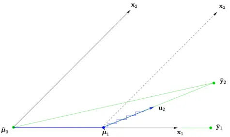
stagewise regression is less greedy by taking η to be small. The differences of

forward selection and forward stagewise regression for p = 2 are illustrated in

Figure 1.1. If the step sizeηis chosen to be very small in stagewise regression, the

procedure can be computationally intensive.

1.3.4

Least angle regression

Least Angle Regression (LARS) [Efron et al., 2004] is a principled and

computa-tionally efficient version of stagewise regression. Similar to stagewise regression,

LARS builds µˆ = Xβˆ at each step, and initialises βˆ= (β1, β2, . . . , βp) = 0. The

procedure starts by finding the variablexj1 that is most correlated withY, andµˆ

proceeds in the direction of this variable until another variable xj2 has the same

amount of correlation with residualr=Y₋µˆ asxj1. LARS then proceeds in the

direction that is equiangular between xj1 and xj2, until another variable xj3 has

(17)

Figure 1.1: Illustration of forward selection, stagewise regression and LARS for

p = 2. y¯₂ is the projection of Y on space spanned by x1, x2, and µˆ0, µˆ1, µˆ2

denote the estimated response at steps 0,1 and 2. The initial response estimate is

ˆ

µ0 = 0, and the residual (i.e., y¯2) has higher correlation with x1, so the LARS

algorithm proceeds in direction of x1 until µ = µˆ1, which is the point where

the residuals y¯₂ ₋ µ have the same correlation with x1 and x2, and then the

algorithm proceeds along the bisector direction (indicated by u2) until µˆ2 = ¯y2.

In contrast, forward stagewise regression takes small step size such that its path

has staircase shape (purple line), and forward stepwise regression proceeds in x1

direction further than LARS until y¯₁, the projection of Y on to x1. [Figure

reproduced from Efron et al., 2004]

then proceeds in the direction that is equiangular between xj1, xj2, xj3. This

process continues until all variables are included.

LARS is computationally efficient since it can produce piecewise linear

solu-tion path with p steps. It can also be adapted to provide the solution path for

some other methods such as Lasso (see Section 1.4.2.2), which significantly

ac-celerates the computation. Finally, the LARS estimator tends to assign highly correlated features with similar coefficient estimates, which is a desirable property.

(18)

1.4

Penalised regression

Conventional variable selection approaches may not be suitable for high-dimensional data. For instance, best subset selection fails to cope with large number of vari-ables, since it is extremely variable due to the nature of discreteness, and com-putation can be prohibitive, because the number of potential sub-models grows exponentially with dimensionality. Greedy algorithms such as forward and back-ward selection can be unstable with high variance due to their discontinuous prop-erty, i.e., a small change in the data can lead to completely different estimates. Penalised likelihood regression methods achieve variable selection in a continuous and computationally efficient way, and suffer less variability. Below, we first pro-vide an introduction to penalised likelihood regression model in general and then describe some specific methods.

1.4.1

Introduction to penalised regression

Penalised regression methods augment the loss function with a penalty term that encodes a structural assumption such as sparsity. Specifically, in penalised

like-lihood regression, instead of maximizing the likelike-lihood function l(β_|Y,X), one

maximises the objective function

M(β) = l(β_|Y,X)₋Pλ(Θ), (1.8)

wherePλ(.)is a penalty function that penalises complex models, andλ >0controls

the degree of penalisation. In linear regression model, it is equivalent to minimising the objective function using RSS as the loss function:

M0(β) =_||Y₋Xβ_||2

2+Pλ(β). (1.9)

Throughout the thesis, we use (1.9) as the objective function for penalised linear

regression. Pλ(β)shrinks some coefficient estimates towards zero, and whenPλ(β)

satisfies certain properties, some of the coefficients are shrunk to exactly zero, leading to a sparse solution.

(19)

λ. The choice of λ can be data-driven, such as minimising information criteria

or through cross-validation. Specifically, when using information criteria, λ is

chosen such that optimal information criteria score is achieved. Common criteria

include AIC, BIC and for ultra-high dimensional data, extended BIC (EBIC) [Chen

and Chen, 2008]. Cross-validation is a technique to evaluate how well model

estimates can be generalised to an independent unseen data set. Specifically for linear regression, in a k-fold cross-validation, the original samples are randomly

partitioned into k subsets of the same size. One subset is treated as validation

data, while the rest of the subsets are treated as training data. The model is fitted on the training data while prediction accuracy is evaluated using the validation

data to give a score. The process is repeatedk times (folds), such that each subset

is used as validation data exactly once. Scores are then averaged across folds to

produce an estimate for out-of-sample prediction accuracy. λ that minimises the

cross-validation prediction error is considered optimal for the model to generalise to an independent dataset.

1.4.2

Penalised regression methods

In this section we introduce several popular penalised regression methods for

high-dimensional data analysis. Below, we will use the following definitions about

variable selection consistency, estimation consistency and prediction consistency.

Letβˆ be an estimate ofβ.

Definition βˆ is a consistent estimate if

ˆ

β₋β_→0,asn_{→ ∞}, (1.10)

Definition βˆ is selection consistent if

P(_{j : ˆβj 6= 0}={j :βj 6= 0})→1,asn → ∞ (1.11)

Definition βˆ is prediction consistent if

(20)

In order to illustrate the main properties of these methods, we show their

behaviour on a toy example. Specifically, data are generated using model (1.1),

with n = 100, p = 500 and σ = 4. The p variables are drawn from multivariate standard normal distribution, and the first five variables have pairwise correlation

ρ = 0.9 with each other, and the remaining variables are independent from each

other, and independent from the first five correlated variables. There are 10

rele-vant variables, i.e., s0 = 10. The five correlated variables have coefficients 1, and

the first five independent variables have coefficients 6, while other variables have coefficients 0. Coefficients can be summarised as follows:

βj =      1 for j = 1, . . . ,5 6 for j = 6, . . . ,10 0 for j = 11, . . . ,500 (1.13)

Penalty level is chosen by 10-fold cross-validation, and for each method we present the number of selected variables and coefficient estimates for the relevant variables.

The results are shown in Table 1.1.

model size

ˆ

β1, . . .βˆ5

(correlated relevant variables)

ˆ

β6, . . .βˆ10

(independent relevant variables)

Ridge 500 0.29, 0.37, 0.45, 0.41, 0.41 0.73, 0.62, 0.66, 0.68, 0.52 Lasso 48 0.00, 0.00, 2.53, 1.72, 0.00 5.24, 5.41, 4.97, 5.33, 4.43 ENet 144 0.00, 0.59, 1.48, 1.21, 0.92 4.13, 3.71, 3.77, 3.79, 3.01 SCAD 8 0.00, 0.00, 0.00, 0.00, 4.30 5.88, 6.44, 5.43, 6.17, 4.87 Adalasso 20 1.29, 0.00, 0.00, 0.00, 2.62 5.25, 6.89, 4.69, 5.39, 5.71 Dantzig 41 0.00, 0.00, 2.78, 1.36, 0.00 5.26, 5.26, 4.88, 5.41, 4.80

Table 1.1: Model size and coefficient estimates for different methods in the toy example. See text for details of data generation. Model size and coefficient

esti-mates of the five correlated relevant variables (βj = 1, j = 1, . . . ,5) and the five

independent relevant variables (βj = 6, j = 6, . . . ,10) are presented. ENet stands

for Elastic Net, and AdaLasso stands for Adaptive Lasso. α for Elastic Net is

(21)

1.4.2.1 Ridge Regression

When strong multicollinearity exists, i.e., some variables can be largely

approxi-mated by others linearly,XT_X _{is (nearly) singular, and the MLE is highly variable}

or not uniquely defined. Ridge Regression [Hoerl and Kennard, 1970] addresses

this problem by adding an l2 penalty, i.e.,Pλ(β) = λ||β||22.

Properties The l2 penalty reduces variation of βˆ by introducing bias through

the penalisation of coefficient magnitudes. Asλincreases, the bias of the coefficient

estimates increases while their variance decreases. It is equivalent to adding λ to

the diagonal elements ofXTX, making it less close to being singular and therefore

improving the stability of the matrix inversion.

With carefully chosen λ, the Ridge estimator outperforms the MLE with

re-spect to prediction, especially when variables are highly non-orthogonal [Hoerl and

Kennard, 1970]. The l2 penalty results in Ridge Regression having a grouping

ef-fect, such that highly correlated variables tend to have similar coefficient estimates

[Zou and Hastie, 2005]. From Table 1.1 the coefficient estimates for the five

cor-related relevant variables are similar to each other thanks to the grouping effect. Ridge Regression is also known to perform well in prediction when many variables are relevant with small coefficients, but is suboptimal when the underlying model

is sparse [see e.g. Ogutu et al., 2012]. Indeed, from Table 1.1 its coefficient

es-timates of relevant variables are significantly underestimated compared to other methods.

Since the l2 penalty is not singular at the origin, Ridge Regression does not

directly perform variable selection. From Table 1.1 we see that Ridge Regression

is the only method that does not perform variable selection, since all p

coeffi-cients have non-zero estimates. With an appropriate thresholding strategy [e.g.,

Shao and Deng, 2012], it can be seen as an alternative. Specifically, the authors

proposed a threshold an = Cn−α for some C > 0 and 0 < α ≤ 1/2, such that

variables with absolute coefficients larger than an are selected to be in the model.

The thresholding enables Ridge Regression to achieve variable selection, and the authors proved that under certain sparsity assumptions, the thresholded Ridge Regression achieves consistency of variable selection, estimation and prediction.

(22)

Computation Ridge Regression has an analytical solutionβˆ = (XT_X₊_λ_I)−1_XT_Y_.

1.4.2.2 Lasso

The Lasso (least absolute shrinkage and selection operator) estimator [Tibshirani,

1996] takes the form given in (1.9) with anl1-norm penalty: Pλ(βj) =λ|βj|. This

shrinks coefficients towards zero, with some set to exactly zero, and λcontrols the

amount of shrinkage and degree of sparsity.

Properties The theoretical properties of the Lasso have been well-studied and are mostly based on asymptotic analysis. We highlight some of the main properties here.

The design matrix X needs to satisfy the irrepresentable condition for

consis-tent variable selection [Zhao and Yu, 2006]. This condition specifies a restriction

on covariance between variables, such that the total amount of any irrelevant vari-ables that can be represented by the relevant varivari-ables is limited, or in other words, irrelevant variables are irrepresentable by the relevant ones. More formally, for a

scalar a, let sign(a) denote the sign of a, such that sign(a) = 1 if a > 0, -1 if

a < 0, or 0 if a= 0. Additionally, for a vector v, let sign(v) denote the vector of

signs of the elements in v. Then, the strong irrepresentable condition is satisfied

if _||Σωc_ωΣ−1

ωωsign(βω)||∞ ≤ 1−τ for some τ > 0, and the weak irrepresentable

condition is satisfied if _||Σωc_ωΣ−1_ωωsign(β_ω)||_∞ < 1. Here, Σ_ω

1,ω2 = 1 nXω1 0 Xω2, ω = _{j : βj 6= 0,1 ≤ j ≤ p}, ωc = {j : βj = 0,1 ≤ j ≤ p}, and || · ||∞ is the

infinity norm. The irrepresentable condition does not hold when X is ill-posed

with strong multicollinearity, which is common in high-dimensional data.

Let λn indicate that λ is a function of sample size n. Under certain

regular-ity conditions with respect to the design, the following holds: if λn/n → 0 and

λn/n

1+c

2 → ∞ for some 0 ≤ c < 1, then the strong irrepresentable condition

implies sign consistency [Zhao and Yu, 2006],

lim

n→∞P(sign( ˆβ) = sign(β)) = 1, (1.14)

which is stronger than selection consistency.

(23)

design, letλn= √λ0_n for someλ0 >0, the probability of Lasso detecting all relevant

variables grows to one in exponential rate with respect to n, while the probability

of estimating an incorrect sign pattern converges to a limit in (0,1). Wainwright

[2009] proves that consistent variable selection of Lasso requires

s0log(p) =o(n), (1.15)

which establishes the relationship between n, p and s0 for variable selection

pur-pose.

Lasso can only select up to n variables, which is not ideal for small n, large s0

problems. Finally, Lasso does not have group selection property, such that it tends to only select a few variables from a group of highly correlated variables, which

is not ideal when many signals are correlated with each other. From Table 1.1

we see that Lasso only manages to pick up two out of the five strongly correlated relevant variables, which illustrates the fact that Lasso has difficulty discovering all the highly correlated relevant variables. When strong multicollinearity breaks the irrepresentable condition as in this case, Lasso fails to achieve consistent variable selection.

For prediction, Lasso can achieve consistency with respect to prediction loss

un-der almost no assumptions [Chatterjee,2013]. λshould typically be larger for

con-sistent variable selection than for concon-sistent prediction, and the prediction-optimal

λcan lead to inclusion of many false positives [Meinshausen and Bühlmann,2006].

From Table 1.1 we see that Lasso performs variable selection such that only 48

variables have non-zero estimates, although due to cross-validation getting λ for

prediction, the model size is overly large.

Computation Lasso optimization can be solved with the generalised gradient

descent approach [Friedman et al.,2010], which is implemented in theglmnet

pack-age. The Lasso problem can also be solved by the LARS algorithm with certain

modification [Efron et al.,2004], for all λ_∈[0,_∞] (see Section1.3.4). Specifically,

in the LARS procedure, while updating µˆ, whenever a non-zero coefficient hits

zero, the corresponding variable is removed from the selected set of variables and the equiangular joint direction is updated. LARS can provide computational

(24)

ef-ficiency when the solution is investigated for many values of tuning parameter λ

[Tibshirani and Taylor, 2011]. The level of regularization λ is usually determined

to minimise cross-validation error in practice.

1.4.2.3 Elastic Net

Elastic Net [Zou and Hastie, 2005] is (1.9) with a convex combination of l1 and

l2 penalty Pλ(βj) = λ1|βj| +λ2βj2 = λ α|βj|+ 1−₂αβj2

, where λ1, λ2 > 0 and

α_∈[0,1]controls the balance of the two (α=1 and α=0 correspond to Lasso and

Ridge Regression respectively).

Properties The l1 penalty guarantees automatic variable selection and

continu-ous shrinkage, while thel2 penalty helps select correlated variables (signal or

non-signal) simultaneously thanks to the group selection property, and it also stabilises

the solution path. From Table 1.1 we see that Elastic Net selects more correlated

variables than Lasso, and coefficient estimates for those correlated variables tend to be reasonably similar in magnitudes due to its group selection property. Its se-lection and estimation behaviour is in between that of Lasso and Ridge Regression,

due to the compromise ofl1 and l2 penalty. In the p > nscenario, Elastic Net can

select more than n variables, in contrast to a maximum of n variables for Lasso.

In the toy example when α= 0.1, Elastic Net selects 144 variables, a value larger

than n = 100. Comparison of Elastic Net penalty and l1, l2 penalties is shown in

Figure1.2. The shape of the Elastic Net penalty is in between that of thel1 and l2

penalties. The edges are strictly convex for both Lasso and Elastic Net penalties, and singularities at the axes (where the contour hits the axes) guarantee their sparse solution.

Computation Elastic Net problem can be converted to Lasso problem with

augmented data. Specifically, let X∗ _{= (1 +} _λ

2)− 1 2 X √ λ2I ! , and Y∗ ₌ Y 0 ! , thenM(λ0,β∗) = _||Y∗ ₋_X∗_β∗_||2 2+λ0||β∗||1, andβˆ(NEnet)=√₁₊1_λ 2 ˆ β∗ _{is the naive}

elastic net solution. To correct extra bias introduced by double shrinkage of naive elastic net (Ridge-type shrinkage followed by Lasso-type shrinkage), scaling is

(25)

304 H. Zou and T. Hastie

β1

β2

Fig. 1. Two-dimensional contour plots (level 1) (---, shape of the ridge penalty; - - - -, contour of the lasso penalty; , contour of the elastic net penalty withαD0:5): we see that singularities at the vertices and the edges are strictly convex; the strength of convexity varies withα

Lemma 1.Given data set.y,X/and.λ1,λ2/, deﬁne an artiﬁcial data set.yÅ,XÅ/by

XÅ_.n₊_p/_×_p=.1+λ2/−1=2 X √_λ 2I , y_.nÅ₊_p/= y 0 :

Letγ=λ1=√.1+λ2/andβÅ=√.1+λ2/β. Then the na¨ıve elastic net criterion can be written

as L.γ,β/=L.γ,βÅ/=yÅ−XÅβÅ2+γβÅ₁: Let ˆ βÅ=arg min βÅ L{.γ,βÅ/}; then ˆ β=√ 1 .1+λ2/ ˆ βÅ:

The proof is just simple algebra, which we omit. Lemma 1 says that we can transform the na¨ıve elastic net problem into an equivalent lasso problem on augmented data. Note that the sample size in the augmented problem isn+pandXÅhas rankp, which means that the na¨ıve elastic net can potentially select allppredictors in all situations. This important property overcomes the limitations of the lasso that were described in scenario (a). Lemma 1 also shows that the na¨ıve elastic net can perform an automatic variable selection in a fashion similar to the lasso. In the next section we show that the na¨ıve elastic net has the ability of selecting ‘grouped’ variables, a property that is not shared by the lasso.

Figure 1.2: Two-dimensional contour plot to compare penalties for Lasso ( . . . ),

Ridge Regression (_−·−) and Elastic Net ( , α= 0.5) [Figure reproduced from

Zou and Hastie,2005]

modification of LARS, the above problem can be efficiently solved by the

LARS-EN algorithm [Zou and Hastie, 2005].

1.4.2.4 SCAD

Lasso-type approaches introduce bias for large coefficients, since they equally

pe-nalise each variable. Smoothly Clipped Absolute Deviation (or SCAD) [Fan and

Li,2001] guarantees the solution to be sparse, continuous, and nearly unbiased for

large coefficients. It uses the following penalty in (1.9):

Pλ(βj) =      λ_|βj|, if |βj| ≤λ −|βj|2−2aλ|βj|+λ2 2(a−1) , if |βj| ∈(λ, aλ] (a+1)λ2 2 , if |βj|> aλ (1.16) where a >2 and λ >0.

(26)

Properties SCAD penalty is a non-convex, quadratic spline function by which small coefficients are shrunk towards zero with a Lasso penalty, while large coeffi-cients are not penalised. The resulting estimator is, unlike Lasso, nearly unbiased

for large coefficients. Fan and Li[2001] and Fan et al.[2004] also show that SCAD

enjoys an oracle property (assuming some regularity conditions) – it is simultane-ously consistent for variable selection and estimation, where the latter is as efficient (asymptotically) as the ideal case when the true model is known in advance. For

further details on the properties of SCAD, see Fan and Lv [2010] and references

therein.

From Table 1.1 we see that thanks to its adaptive penalty, SCAD penalises

large coefficients (βj = 6for j = 6, . . . ,10) less than Ridge Regression, Lasso and

Elastic Net such that corresponding estimation is more accurate. Also its model size is significantly smaller than Lasso and Elastic Net, which is related to its oracle property for variable selection.

Computation The SCAD problem can be solved by an iterative procedure or

one-step procedure [Fan and Li,2001], with appropriately chosen initial estimators.

We fixato be 3.7, and tuneλby cross validation, which are recommended byFan

and Li [2001]. a= 3.7minimises Bayes risks from an empirical point of view, but

it can also be tuned via cross-validation.

1.4.2.5 Adaptive Lasso

Adaptive Lasso [Zou, 2006] also aims to adaptively impose penalties on different

coefficients, such that large coefficients are less penalised than small ones. It uses

the following penalty in (1.9)

Pλ(βj) = λwj|βj|, (1.17)

where wj >0 is a known weight for variable j.

Properties When wj has the form _|_β_ˆ1

j|τ for some τ > 0 and

ˆ

βj is a root-n

consistent estimate of βj (i.e., βˆj −βj = Op(n−1/2)), adaptive Lasso also enjoys

(27)

penalised since a large penalty will be placed for coefficients with small initial

estimates; similarly, large coefficients tend to be un-penalised. From Table 1.1,

we see that, compared to Lasso, Adaptive Lasso gives a more parsimonious model with 20 selected variables. It also achieves better estimation of large coefficients

(βj = 6) compared to Lasso and Elastic Net, which equally penalise all variables.

Computation Zou [2006] suggests to use least squares estimates as initial es-timates, unless strong multicollinearity exists, in which case Ridge estimate is preferred due to its stability. Lasso estimate is also a common choice for the initial

weights (for example, seeKrämer et al.[2009]), since it is root-n consistent [Knight

and Fu, 2000]. We use Lasso estimates as the initial estimates for adaptive Lasso

throughout the thesis. The adaptive Lasso problem can be converted to a standard Lasso problem, which can then be solved by the LARS algorithm. In particular,

let x∗

j = xj

wj, then the Lasso problem

ˆ β∗ _{= arg max} β∗ || Y₋Pp_j₌₁x∗ jβ ∗ j||22+λ||β ∗ ||1

can be solved to give the adaptive Lasso estimate βˆj(AdaLasso) =

ˆ βj

∗

wj, j = 1. . . p.

1.4.2.6 Dantzig Selector

The Dantzig Selector estimator [Candes and Tao, 2007] takes a different form to

that in (1.1), namely: ˆ β_λ = argmin β kβ_k1 :kXT (Y−Xβ)k∞ ≤λ , (1.18)

Properties The Dantzig Selector and the Lasso are closely connected as

dis-cussed inBickel et al.[2009], and under certain conditions onX, Lasso and Dantzig

Selector provide the same solution [James et al., 2009; Meinshausen et al., 2007].

From Table1.1 we see in the toy example, Dantzig Selector and Lasso have similar

model size and similar coefficient estimates for relevant variables.

It is proved that, in noiseless case where Y = Xβ, if the design matrix X

obeys the uniform uncertainty principle (UUP), Dantzig Selector can achieve exact recovery with some regularity assumptions on design. Loosely speaking, the UUP

requires that any subset of columns of X with cardinality smaller than s0 can be

(28)

error E_||β(oracle)₋β_||2 2 ≥

1 2 ×

P

imin(βi2, σ2), and Dantzig Selector can achieve

this ideal estimation error within a factor ofO(logp).

Computation The Dantzig Selector problem can be solved with linear program.

1.4.2.7 Other methods

There are numerous other penalised regression methods for high-dimensional data.

For example, the minimax concave penalty (MCP) [Zhang, 2010] also achieves

sparsity, continuity and near unbiasedness for large coefficients like SCAD. It min-imises maximum concavity of penalised loss function, with restrictions on un-biasedness and variable selection. There are also penalised regression methods

designed for specific types of data. When variables can be sorted into K groups,

with pk the size of group k (k = 1. . . K), group Lasso [Yuan and Lin, 2006]

uses Pλ(β) = λPK_k₌₁√pk||β(k)||2, where β(k) are the coefficients of variables

in group k. Coefficients from each group share the same level of penalty. To

introduce sparsity within a group, Friedman et al. [2010] suggest adding an l1

term into the group Lasso penalty. Fused Lasso [Tibshirani et al., 2005] is

desir-able for problems where varidesir-ables can be ordered meaningfully. The penalty is

Pλ(β) = λ1

Pp

j=1|βj|+λ2

Pp

j=2|βj −βj−1| for some λ1, λ2 > 0. The l1 penalty

on successive differences of coefficients introduces corresponding sparsity, and con-sequently local constancy of estimation. This is desirable for interpretation in certain scientific problems. There are also variants of methods aiming to improve

the selection and predictive performance. For example, Zeng and Xie [2012] add

an l2 penalty to SCAD to obtain the group selection property, while preserving

unbiasedness, continuity, and sparsity. The authors showed that this approach stabilises variable selection in multicollinearity settings, with enhanced prediction accuracy.

(29)

1.5

Bayesian linear regression

1.5.1

Bayesian inference

Bayesian inference is based on Bayes’ theorem, and uses probability distributions to explicitly quantify the uncertainty in inference. Bayesian methods assume pa-rameters to be unknown random variables instead of fixed values, and assign prior distributions to parameters, enabling prior knowledge to be specified. A full prob-ability model is set up with a joint distribution for observed and unobserved quan-tities, and a posterior distribution of unobserved quantities of interest is obtained, conditional on the observed data. Inference is carried out using these posterior distributions.

Formally, let Θ be the unknown parameters of interests, and D the observed

data. A prior distribution for Θ, p(Θ) quantifies prior information on the

pa-rameters before observing the data, and p(D_|Θ) is the likelihood function. The

posterior distribution ofΘ given D is then calculated as

p(Θ_|D) = p(D|Θ)p(Θ)

p(D) , (1.19)

where p(D) is the marginal likelihood of the observed data, marginalised over Θ,

p(D) =

Z

Θ

p(D_|Θ)p(Θ)dΘ. (1.20)

The distribution ofΘ can have its own parameter(s)τ, called hyperparameter(s),

i.e., Θ _∼ p(Θ_|τ). τ can be a tuning parameter set by the user or can also be

considered as a random variable and have its own prior.

1.5.2

Bayes factor

The Bayes factor is widely used for Bayesian model comparison. It is the ratio of the marginal likelihood of two competing models. Unlike classical likelihood ratio where parameters are maximised under corresponding models, they are integrated out. The Bayes factor quantifies the relative evidence of the competing models, and facilitates model selection.

(30)

Formally, in a model selection problem based on the observed data D, where

one needs to choose from two candidate models M1 and M2, with parameters Θ1

and Θ2 respectively, the Bayes factor is defined as

where p(M1) and p(M2) are the prior probabilities of M1 and M2. The Bayes

factor is the ratio of marginal likelihood of two model specifications, taking into account the uncertainty in parameters, in contrast to classical likelihood ratio,

LR= l( ˆΘ1|D, M1)

l( ˆΘ2,|D, M2)

, (1.22)

which is the ratio of two likelihood functions, maximised with respect to their

parameters, and Θˆ1 and Θˆ2 are MLEs.

When M1 and M2 are equally likely a priori, the Bayes factor can also be

simplified as BF = p(M1|D)

p(M2|D), which is the ratio of posteriors of the two models.

BF >1 means model M1 is more supported by the data than M2, while BF <1

means modelM2 is more supported. The Bayes factor does not depend on specific

values of the parameters, and a sparsity prior for Θ can be incorporated into the

Bayes factor to penalise complex models.

BIC can be used to approximate the Bayes factor [Kass and Raftery, 1995].

Specifically in linear regression, letM2 andM2 be two different models, then with

certain priors onβ’s, the Bayes factor of modelM1 versusM2can be approximated

as BF12 ≈ PBIC(D|M1) PBIC(D_|M2) =exp(∆BIC21 2 ), (1.23)

whereBIC(Mi) =−2logl( ˆβ

i

|D, Mi)+kilogn,βˆ

i

andki being the MLE and degree

of freedom of modelMi; PBIC(Mi) = exp(−BIC₂(Mi)); and ∆BIC21 =BIC(M2)−

(31)

1.5.3

Bayesian linear model

In a Bayesian linear regression model, β and σ2 _{in (}_1.1_{) are treated as unknown}

random variables, and inferences are made based on the posterior distribution of

β and σ2 _{given the data. Let}_{Θ = (}_β_{, σ}2₎ _and _p_(Θ) _{denote the prior distribution}

overΘ. Then the posterior distribution over Θis

p(Θ_|X,Y) = p(Y|X,Θ)p(Θ)

p(Y_|X) , (1.24)

where

p(Y_|X,Θ) =N(Xβ, σ2I). (1.25)

Since the posterior is a density instead of a point estimate, the level of associated uncertainty can be quantified using, for example, credible intervals.

In order to calculate the posterior probability, one must calculate p(Y_|X) =

R

p(Y_|X,Θ)p(Θ)dΘ, which is not available in closed form in general. If that is

the case, numerical approaches are required to evaluate the integral, which can be computationally intensive. The exception is when the prior is conjugate, which

means that the prior and posterior ofΘhave the same parametric form. Conjugate

priors result in a closed-form solution for the integral and provide computation

efficiency. Specifying the prior distribution for Θ is a challenging task, and a

poor choice of prior distribution can lead to inaccurate posterior distribution, and consequently inferior model performance, especially when the sample size is small.

In Bayesian linear regression, a common conjugate prior for Θ is called the

normal inverse gamma (NIG) distribution. It assumes β_|σ2 _{follows a multivariate}

normal distribution, and σ2 _{follows an inverse-gamma distribution. Formally, the}

joint distribution of β and σ2 _is

p(β, σ2) =p(β_|σ2)p(σ2) = N(β_|µ, σ2V)IG(σ2_|a, b), (1.26)

whereµ,V, a >0, b >0are hyperparameters, and the inverse-gamma distribution

IG(σ2_|_{a, b}₎ _{has the form}

IG(σ2_|a, b) = b

a Γ(a)(σ

2₎−(a+1)_exp₍

(32)

where Γ(.) is the Gamma function. Due to conjugacy, applying Bayes’ theorem

(1.24), the joint posterior of (β, σ2_{) is also a NIG distribution,}

p(β, σ2_|Y,X) =N IG(µ?_,_V?_{, a}?_{, b}?₎_, _(1.28) where µ? _{= (V}−1 +XTX)−1(V−1µ+XTY) V? = (V−1+XTX)−1 a? =a+n/2 b? =b+ 1 2(µ T_V−1 µ+YTY₋(µ?₎T_(V?₎−1 µ?₎_. (1.29)

σ2 or β can be integrated out from the joint distribution to obtain marginal

dis-tribution of the other. A point estimate of parameters can be obtained by sum-marising the distribution, and the distribution explicitly reveals the uncertainty of the parameters.

1.5.4

Bayesian Ridge Regression

Ridge Regression can deal with p > n scenarios, and is computationally efficient

due to its closed-form solution. Ridge Regression can be formulated in a Bayesian way. Specifically, the Bayesian representation of Ridge Regression is as follows:

p(Y_|X,β, σ2) =N(Xβ, σ2I) β_|σ2, λ_∼N0,σ 2 λ I σ2 _∼IG(a, b), (1.30)

where λ >0 is a tuning parameter controlling the degree of shrinkage. Note that

this prior specification of σ2 and β is the NIG prior (1.26) for linear model with

µ=0 and V = 1_λI. Applying Bayes’s theorem (1.24) and integrating out σ2, the

(33)

[Denison et al., 2002] p(β_|X,Y) =M V St2a+n( ˆβ, b+ 1₂(YT_Y₋_β_ˆT₍_λ_I₊_XT_{X) ˆ}_β₎ a+ n 2 (XTX+λI)−1), (1.31)

where M V Stν(µ,Σ)has probability density function

p(x) = Γ[(ν+p)/2] Γ(ν/2)νp/2_πp/2_|_Σ_|1/2[1 + 1 ν(x−µ) T_Σ−1 (x₋µ)](ν+p)/2, (1.32)

and p is the dimension of x. The mean βˆ = (XTX+λI)−1XTY is identical to

frequentist Ridge Regression estimate in Section 1.4.2.1. The hyperparameters a

and b for the prior on σ2 are typically chosen to be non-informative, i.e., a, b are

close to zero, and as in frequentist Ridge Regression, the posterior distribution

of β’s is shrunk towards zero. The marginal distribution of Y also follows a

multivariate Student t-distribution [Denison et al.,2002], i.e.,

p(Y) = Z P(Y_|β, σ2)P(β, σ2)dβdσ2 =M V St2a(0, b a(I+ XXT λ )) (1.33)

1.6

Ensemble learning methods

Ensemble learning aims to improve machine learning methods by combining dif-ferent models in a strategic way. While ensemble learning requires more compu-tations than a single model, it can obtain better model performance than any of the constituent models alone. It is known that diversity among candidate mod-els in ensemble learning helps yield better results, and many ensemble learning

methods seek to increase such diversity [Brown et al., 2005]. Some common

en-semble learning methods include bootstrap aggregation [bagging,Breiman,1996],

boosting [Freund and Schapire,1999] and stacking [Wolpert,1992]. Below we give

(34)

1.6.1

Bootstrap aggregation

Bootstrap aggregation (bagging) is one of the most intuitive ensemble based meth-ods, where diversity of models (i.e., differences among models) is obtained by

bootstrapping the training data. That is, new training data samples of size n are

randomly drawn with replacement from the full data. For large n, each bootstrap

sample is expected to have _∼63.2% of the unique samples of the full data, while

the rest are duplicates. Models are then fitted to each bootstrap sample before they are combined through averaging the output. Each model has a high variance and

low bias, and combining them reduces the variance. According to Breiman [1994,

1996], bagging can improve the instability in procedures such as classification and

regression trees, and variable selection in linear regression.

Bootstrap-enhanced Lasso

An interesting attempt to combine bagging and penalised linear regression is called

Bootstrap-enhanced Lasso, or Bolasso for short [Bach,2008], which runs Lasso on

several bootstrap samples of the training data, and the intersect of the selected variables of bootstraped Lasso are defined as the relevant variables. Under certain conditions, Bolasso leads to consistent model selection, and in general, Bolasso can fix the instability of Lasso and correctly retrieve the sparsity pattern when Lasso’s consistent selection conditions are not satisfied. Bolasso enhances Lasso’s variable selection performance and is consistent under more general assumptions.

Stability Selection

Bolasso is mainly designed for low-dimensional data, and its properties are proved

under the condition that p is fixed with respect to n. Stability Selection [

Mein-shausen and Bühlmann,2010] is a very general method combining subsampling and

variable selection methods, with the aim of providing finite sample false positive

error control. Specifically,M random data subsamples of size ˜n < nare generated

by sampling without replacement. n˜ is typically chosen to be _bn/2_c or _b0.632n_c,

which closely resemble the bootstrap. Applying a variable selection procedure,

with regularization parameterλ, to these datasets gives a scoreΠˆλ,j indicating the

(35)

probability. Let Λ denote the set of considered values for the regularization pa-rameter. Then, a set of “stable variables” is obtained by choosing those variables

that have selection probabilities larger than a cutoff value πthr ∈ (0,1) for any

λ_∈Λ.

In contrast to the penalised regression methods and Bolasso, Stability Selection

does not require setting of the parameterλ, but instead requires the cutoff πthr to

be chosen (Bolasso fixes πthr to be 1). Meinshausen and Bühlmann [2010] provide

theoretical results showing howπthrcan be chosen to achieve a user-specified upper

bound V˜ on the expected number of false positives _E[V], assuming a fixed set of

regularization parameters Λ. Alternatively, the user can fix πthr and then the

theory shows howΛshould be chosen to achieve the desired upper bound on_E[V].

In this thesis we use the Lasso as the variable selection procedure with Stability Selection.

1.6.2

Random forest

Decision tree

A decision tree seeks to predict the unseen response based on input variables. It can be presented by a tree structure consisting of nodes and branches. The decision tree model is built in a structured way, where the data samples are segmented into subgroups through a series of decisions, and each internal node corresponds to a test on an input variable. The model starts with all samples in one node, called the root node, and the first split is made with one variable, such that samples are partitioned among its child nodes, according to the decision rule for the variable. Branches connecting an internal node and its child nodes represent the decision rule outcomes. Then child nodes follow similar procedure to further segment the data recursively, until leaf nodes are reached where further splits are not possible or will not improve the model fit. At each split, the model fit is evaluated by homogeneity in class labels/observed responses of resulting child nodes, and one chooses the split that increases such homogeneity. A leaf node represents a class label/observed response or a distribution of the class labels/observed responses.

Greedy approach is typically applied for construction of a decision tree. The most significant variable is chosen to be the root node, and more significant

(36)

vari-x(1) x(2) response 1 response 0 1 x(3) response 1 response 0 0

Figure 1.3: An illustration of decision tree

ables are closer to the root node. The significance of a variable can be calculated using information theory criteria (for example, a measure of node impurity de-crease). Prediction of class label for new data is made based on the paths of decisions from the root node to leaf nodes.

Figure 1.3 illustrates the structure of a decision tree. x(1)_,_x(2) _and _x(3) _are

binary variables taking values zero and one, and they are ranked by their

signifi-cance. The node at top is the root node, and represents a test on x(1) _{being zero}

or one. A split is made to represent two different outcomes of this test. Depending

on the test result, one tests the next variable (x(2) _or _x(3)_{) and further split the}

data, reaching the leaf nodes at bottom representing the observed responses. At each split, the goal is to increase the homogeneity in responses among child nodes. Classification trees and regression trees are two common types of decision tree, where predicted outcome is categorical for classification trees and continuous for regression trees.

Random forest

Random forests [Breiman, 2001] are an ensemble learning method designed for

classification and regression, among other tasks. The idea is to construct a series of decision trees, and the output is an average of the individual decision trees. The random forest method is known to correct the overfitting problem of the ordinary

(37)

decision tree method [Hastie et al.,2008]. Each individual tree may be subject to increased bias in estimation and less interpretability, but the final model in general improves method performance significantly.

Random forest involves subsampling of samples and variables. B trees are

constructed with B bootstrapped training data, and to further decorrelate the

trees, at each split of an individual decision tree, a sample of m < p randomly

chosen input variables are considered as split candidates. By doing so, variables have a more uniform chance to be selected, instead of most trees selecting the same set of strong variables, causing trees to be highly correlated, with high variance.

Note that if we choose m=p, random forest is the same as bagging, and using a

small value of m can be useful when strong multicollinearity exists.

1.6.3

Random Lasso

Random Lasso [Wang et al., 2011] is a variable selection method motivated by

random forest, aiming to solve some of the issues of Lasso. Specifically, Lasso does not have group selection property under strong multicollinearity, especially

when coefficients of correlated variables have different magnitudes or signs [Wang

et al., 2011]; Lasso has a limit on the number of selected variables, which could be

undesirable when a large number of variables are relevant.

Random Lasso consists of two steps and can be summarised as follows:

Step 1. Calculate importance measure

1a. For b1 = 1, . . . B, do:

(i) Draw a bootstrap sample by sampling with replacement from full data

(ii) Randomly selectq1 variables from the bootstrapped samples and apply Lasso

to these variables to obtain coefficient estimatesβ˜(b1)

j , j = 1. . . p. Coefficients

for those not among the q1 variables are set to be zero

1b. The importance measure ofxj is calculated asIj =|

PB

b₁₌₁β˜j

(b₁₎

(38)

Step 2. Select variables

2a. For b2 = 1, . . . B, do:

(i) Draw a bootstrap sample by sampling with replacement from full data

(ii) Randomly selectq2 variables from the bootstrapped samples, with selection

probability ofxj proportional to its importance measure Ij. Apply Lasso to

these variables to obtain coefficient estimates βˆj

(b2)

, j = 1. . . p. Coefficients

for those not inq2 variables are set to be zero

2b. The final estimator is βˆj =

PB

b₂₌₁βˆj

(b₂₎

B . Wang et al. [2011] suggest to set

the threshold on magnitudes of coefficient estimates to be 1/n, such that those

variables with _|βˆj|<1/n are removed from the model.

Sampling of variables in Step 1a and 2a breaks down the correlation structure, such that highly correlated variables are selected in different candidate models. In penalised linear regression choosing the right amount of penalisation is notori-ously difficult, especially for high-dimensional data, and there may not be a single

penalty level that can perfectly recover the sparsity pattern [Meinshausen and

Bühlmann, 2010]. Random Lasso applies Lasso on different candidate models,

with different penalty levels; the results are summarised across candidate models, with more stable parameter estimation. The number of selected variables is no

longer limited by n. q1 and q2 are tuning parameters, and Wang et al. [2011]

suggest using cross-validation to find optimal q1 and q2, by repeated application

of Random Lasso, which can be time-consuming.

1.7

Performance metrics

Prediction. To assess predictive performance we introduce two metrics. In

Chap-ters2and 3, predictive performance is compared across different scenarios. In any

simulation scenario, we generate a test data of size ntest, and compare the

(39)

error (RMSE), calculated as

RMSE =_kytest−yˆ||2/√ntest, (1.34)

where yˆ = Xtestβˆ, ytest and Xtest are the test responses and design matrix

re-spectively, and βˆ are the coefficient estimates obtained using the training data.

This metric implicitly involves the impact of error terms, which is important when

comparing among datasets with different noise levels. In Chapter4and 5,

predic-tive performance is evaluated within each scenario, and we use mean squared error

(MSE) as defined inTibshirani[1996], i.e., MSE=(βˆ−β)TV(βˆ−β), whereVis

the population covariance matrix ofX. This metric excludes the influence of error

terms, such that the contrast of prediction performance is clearer among methods.

Variable selection. For assessment of variable selection, we use true positive rate (TPR) and positive predictive value (PPV)

TPR = TP

TP + FN ∈[0,1] PPV =

TP

TP + FP ∈[0,1]. (1.35)

where TP, FP, and FN are the number of true positives, false positives, and false

negatives respectively, with respect to the true underlying model γ. We further

define false positive rate (FPR) as

FPR = FP

FP + TN ∈[0,1], (1.36)

where TN is the number of true negatives.

Variable ranking. For ranking, we assess performance using the partial area under the receiver operating characteristic curve (pAUC). A receiver operating characteristic (ROC) curve shows the performance of binary classification as the

discrimination threshold varies. Specifically, after ranking p variables from the

most important to the least important, take the top k important variables and

calculate FPR and TPR. The ROC curve is TPR values plotted against FPR

val-ues ask varies from 1 top. The area under the ROC curve (AUC) quantifies how

(40)

the (rescaled) AUC score with the restriction on FPR to be smaller than certain threshold. Both AUC and pAUC are between 0 and 1. We use pAUC to

evalu-ate ranking in Chapter 2 and 3, since for high-dimensional data we are typically

interested in those high-ranked variables.

1.8

Thesis overview

The thesis is organised as follows. In Chapter 2 we present a large-scale

com-parison of high-dimensional regression methods, where we systematically consider

the influence of various factors on several widely-used methods. In Chapter3, we

extend the simulations in Chapter2to investigate some further questions with

re-spect to model assumptions and parameter tuning. In Chapter4we propose a novel

variable selection method called STructural RANDomised Selection (STRANDS), which follows the spirit of random Lasso. It uses repeated subsampling of vari-ables to reduce dimensionality before variable selection, and takes into account

the correlation structure of the data. In Chapter 5 we propose another method

combining Bayesian Ridge Regression and forward selection, to improve the

pre-diction performance of Ridge Regression in sparse settings. Finally, in Chapter 6

we summarise and discuss the main conclusions, and point out potential directions for further study.

(41)

Chapter 2

Systematic comparison of penalised

linear regression methods

In this Chapter we present a large-scale simulation study systematically comparing six popular penalised regression methods in high-dimensional settings. We assess their comparative performance with respect to ranking, prediction and variable

selection, using data with various characteristics. In Chapter 3 we extend this

comparison study to explore additional topics with respect to model assumptions and parameter specifications.

2.1