Scaling Populations of a Genetic Algorithm for Job
Shop Scheduling Problems using MapReduce
Di-Wei Huang† and Jimmy Lin‡ Department of Computer Science† and the iSchool‡
University of Maryland College Park, MD 20742 Email:{dwh, jimmylin}@umd.edu
Abstract—Inspired by Darwinian evolution, a genetic algo-rithm (GA) approach is one popular heuristic method for solving hard problems such as the Job Shop Scheduling Problem (JSSP), which is one of the hardest problems lacking efficient exact solutions today. It is intuitive that the population size of a GA may greatly affect the quality of the solution, but it is unclear what are the effects of having population sizes that are significantly greater than typical experiments. The emergence of MapReduce, a framework running on a cluster of computers that aims to provide large-scale data processing, offers great opportunities to investigate this issue. In this paper, a GA is implemented to scale the population using MapReduce. Experiments are conducted on a large cluster, and population sizes up to107 are inspected. It is shown that larger population sizes not only tend to yield better solutions, but also require fewer generations. Therefore, it is clear that when dealing with a hard problem such as JSSP, an existing GA can be improved by massively scaling up populations with MapReduce, so that the solution can be parallelized and completed in reasonable time.
I. INTRODUCTION
In solving hard problems where there lacks efficient exact solutions, heuristic approaches, including genetic algorithms (GAs) [1], simulated annealing [2], and tabu search [3], have become popular alternatives. Among them, GAs can be easily parallelized to scale its computing ability because of its intrin-sic parallelism, and hence offer great potential toward solving hard problems. GAs represent potential solutions by strings of symbols, or linear chromosome, and simulate the process of natural selection, crossover, and mutation among a population of chromosomes, as inspired by Darwinian evolution. Fitnesses of chromosomes are assessed based on the quality of the solutions they represent, and the fitter chromosomes are given higher probability of survival and reproduction. In this manner, a good solution is likely to be evolved after a number of generations.
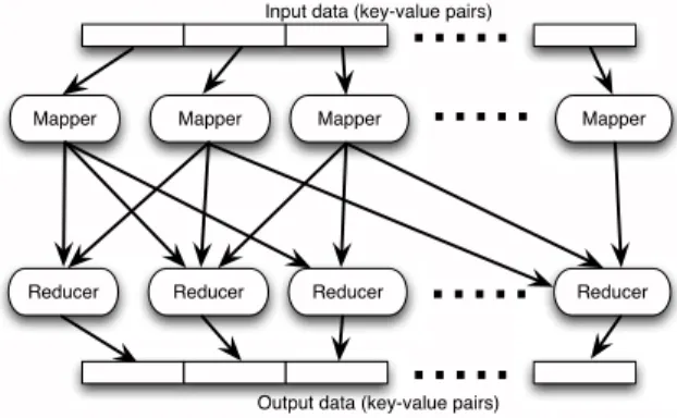
The emergence of the MapReduce framework [4] provides new opportunities to empower GAs with the ability to handle large populations (e.g., millions of individuals). Responding to the need to process huge volumes of data over the growing Internet, MapReduce was designed to support parallel large-scale data processing on a cluster of commodity hardware, which is also known as cloud computing. It aims to provide seamless scalability such that as more machines are added to the cluster, computing capability grows almost linearly. As shown in Figure 1, the framework consists of two types of
Mapper Mapper Mapper Mapper
Reducer Reducer Reducer Reducer
...
...
Input data (key-value pairs)
...
Output data (key-value pairs)
...
Fig. 1. The architecture of the MapReduce framework
components: the mappers and the reducers, which execute map and reduce tasks by invoking user-defined map and
reduce functions, respectively. Each mapper and reducer can be located on separate machines. In a MapReduce job, each mapper processes a portion of the input data in the form of key-value pairs, where each pair is sent as input to the map function. The map function produces zero or more intermediate key-value pairs. These intermediate data are then shuffled, sorted, and sent to the reducers. How these intermediate data are dispatched is controlled by another user-defined component called thepartitioner. The reducers process the intermediate data and output key-value pairs as the final results. The intermediate data sent to a reducer are aggregated and sorted by the keys, where the reduce function is called once for every key. As proposed in [5] and [6], GAs can be fitted into this framework by computing each generation as a separate MapReduce job. Since MapReduce can handle input data of large sizes (e.g., terabytes and even petabytes), it is possible to encode the population of GAs as the input/output data, and benefit from a large population.
To assess the ability of GAs with large populations, the Job Shop Scheduling Problem (JSSP) is chosen as the target problem to be solved. It has drawn much attention not only for its practical applications in operation research, but also for its computational complexity. The objective is to schedule
∣𝐽∣ jobs on ∣𝑀∣ machines such that the makespan, i.e., the
overall time needed to complete all jobs, is minimized. Each job consists of an ordered list of operations, each of which requires being processed by a certain machine for a certain uninterrupted duration. The ordering of operations represents precedences or dependencies among them. Typically, each job contains ∣𝑀∣ operations requiring different machines. Two constraints must be satisfied when scheduling an operation of duration𝑑at time𝑡: (1) all precedent operations are completed before𝑡; (2) no other operations are scheduled to the required machine from 𝑡 to 𝑡+𝑑. The Traveling Salesman Problem (TSP), a well known strong NP-complete problem, is a special case of JSSP [7]. Therefore, JSSP is much harder than TSP and is among the hardest combinatorial optimization problems. Since there are no efficient exact solutions to date, a heuristic approach is needed.
In this study, a GA with massive populations for solving JSSP is implemented using MapReduce. The GA is non-trivial in that it includes encoding/decoding chromosomes, building schedules, performing local searches, handling tournament-base selections, and processing non-random crossover. As it has been suggested by theoretical research [8], [9] that GAs with large population sizes are advantageous in solving hard problems, our GA for JSSP is given massive populations and run on a large cluster. The experimental results show the effects of having massive populations, and confirm that large populations indeed help in finding good solutions. Another experiment is conducted to show that execution time decreases as the size of the cluster grows.
To our knowledge, this is the first implementation of genetic algorithms in MapReduce that takes advantage of state-of-the-art techniques [10]–[14] to solve challenging real-world problems. Although genetic algorithms have previously been proposed for MapReduce [5] [6], the previous work tackled a far simpler problem and lacked many features of modern GA techniques. Use of MapReduce allowed us to explore popula-tion sizes that are significantly larger than typical experiments, and revealed interesting tradeoffs between population sizes and number of generations.
II. ALGORITHMS
This section describes in detail the algorithms used in this paper and how they are implemented in MapReduce. A. Representation
The operation-based representation is adopted [10], [11] to encode and decode the chromosomes. Consider a set of jobs
𝐽={0,1,2, ...}, where each job𝑗∈𝐽contains𝑁𝑗operations (𝑗= 0,1, ...,∣𝐽∣−1). A chromosome contains∑𝑗∈𝐽𝑁𝑗genes that are job names (i.e., members of 𝐽), where each job 𝑗 appears exactly 𝑁𝑗 times. The job name appearing at each gene represents an operation that belongs to the job, where the actual operation is determined by the order of occurrence of that job name, i.e., the𝑘th occurrence of job 𝑗 represents the𝑘th operation of𝑗. For example, with 𝐽 = 2 and𝑁0 =
𝑁1= 3, a chromosome may look like:
[0,0,1,1,0,1]
where the first operation of job0comes first, followed by the second operation of job0, followed by the first operation of job1, and so on. Notice that any permutations of the genes will always yield valid schedules if the operations are added to the schedule in the order of their appearance in the chromosome. The data structure used to store an individual of the GA is shown in Figure 2. This key-value structure is used as the input, the intermediate, and the output data of MapReduce. The key part contains an ID ∈ [0,1) assigned to each individual uniformly at random, and the value part contains a makespan value, a generation value, and the chromosome. The makespan value stores the length of the schedule implied by the chromosome, that is, the length of time between the execution of the earliest operation and the completion of the latest one. The fitness can be evaluated directly through the makespan value, where a lower makespan value represents a fitter individual. The generation value facilitates tracing of evolution by storing the number of generations descended from the original population. Finally, the chromosome is stored as an array of integers.
ID Makespan Generation Chromosome
Key Value
double int int int[]
Fig. 2. The key-value structure to store an individual
B. The genetic algorithm
The main GA is implemented in the MapReduce frame-work where each generation of the GA is performed by a MapReduce job. The data structure shown in Figure 2 is used as the input and output key-value pairs of both the map and reduce phases. The map phase evaluates the fitnesses of the population, where the schedules are built according to the chromosome, and local search is performed to find the makespans. The fittest individual is recorded. The partitioner dispatches the resulting individuals to random reducers by referring to their randomly generated IDs. The reduce phase processes selection and crossover, and produces a new gen-eration population as the output. After the new population has been generated, a new MapReduce job is created for this new generation. This process is continued until a satisfactory solution, if not optimal, to the JSSP is found.
1) Mapper: Fitness Evaluation: The algorithm for the map phase is shown in Algorithm 1, which aims at evaluating the fitnesses (i.e., the makespans) of an individual. Themap
function is invoked once per individual in parallel on multiple mappers. The mapper first obtains an ordered list of operations by decoding the chromosome. A schedule is then built based on the list, where each job in the list is placed on the schedule at the earliest possible time. A local search is performed to fine-tune the resulting schedule [13]. First, the critical path of the schedule is identified as blocks of continuous operations. For each block, if swapping the first two operations or the
Algorithm 1Themapfunction of a single generation of the GA. An ID is required as the key, and an individual is required as the value, as shown in Figure 2.
functionmap(𝑘𝑒𝑦,𝑣𝑎𝑙𝑢𝑒)
begin
𝑜𝑝𝐿𝑖𝑠𝑡←decode(𝑣𝑎𝑙𝑢𝑒.𝑐ℎ𝑟𝑜𝑚𝑜𝑠𝑜𝑚𝑒); foreach operation 𝑜𝑝in𝑜𝑝𝐿𝑖𝑠𝑡do
comment: add to schedule at earliest available spot
𝑠𝑐ℎ𝑒𝑑𝑢𝑙𝑒.add(𝑜𝑝); od 𝑠𝑐ℎ𝑒𝑑𝑢𝑙𝑒.local search() 𝑣𝑎𝑙𝑢𝑒.𝑚𝑎𝑘𝑒𝑠𝑝𝑎𝑛←𝑠𝑐ℎ𝑒𝑑𝑢𝑙𝑒.getMakespan(); output(𝑘𝑒𝑦, 𝑣𝑎𝑙𝑢𝑒); if𝑏𝑒𝑠𝑡.𝑚𝑎𝑘𝑒𝑠𝑝𝑎𝑛 > 𝑣𝑎𝑙𝑢𝑒.𝑚𝑎𝑘𝑒𝑠𝑝𝑎𝑛 then𝑏𝑒𝑠𝑡←𝑣𝑎𝑙𝑢𝑒; fi end finalization output(null, 𝑏𝑒𝑠𝑡);
last two operations yields a shorter makespan then accept it, otherwise undo the swapping. Notice that swapping the first two operations or the last two operations will not improve the schedule, and thus can be omitted. Once a new schedule is obtained by swapping operations, local search is performed again on the new schedule until no improvement can be made. The mapper then outputs the individual with the makespan updated.
In addition to evaluating and outputting individuals, each mapper keeps track of the best individual it has seen. At the end of the mapper’s lifecycle, the best individual is emitted with the ID set to a special valuenull.
𝑟𝑒𝑑𝑢𝑐𝑒𝑟←
{
0, if𝐼𝐷=null
ℎ(𝐼𝐷)%𝑟, otherwise (1)
2) Partitioner: The partitioner assigns the individuals emit-ted from the mappers to the reducers according to the IDs, as characterized by (1), whereℎ(⋅) is a hash function and 𝑟 is the number of reducers. The nullIDs are always sent to the first reducer (i.e., reducer #0). The first reducer is therefore responsible for comparing the best individual from different mappers, and determining the best of the best individual across the whole population. Otherwise, normal IDs are used as input to a hash function to determine which reducer to send to. Since IDs are generated at random, each individual is sent to a random reducer.
3) Reducer: Selection and Reproduction: The algorithm for the reduce phase is shown in Algorithm 2, which selects good individuals and produces descendants by crossing over their chromosomes. The reduce function is invoked once per individual ID in parallel on multiple reducers. The first reducer, i.e., reducer #0, which receives the best individuals from each mapper, records the best among them. This is the best solution found in this generation of the GA. In the following, an approximation of tournament selection is
Algorithm 2 Thereduce function of a single generation of the GA.
functionreduce(𝑘𝑒𝑦,𝑣𝑎𝑙𝑢𝑒𝑠)
initialization 𝑐𝑜𝑢𝑛𝑡←0; 𝑠←5;
begin
if𝑘𝑒𝑦=null then𝑏𝑒𝑠𝑡←arg min𝑣∈𝑣𝑎𝑙𝑢𝑒𝑠𝑣.𝑚𝑎𝑘𝑒𝑠𝑝𝑎𝑛; print(𝑏𝑒𝑠𝑡); return; fi for each𝑣𝑎𝑙𝑢𝑒in𝑣𝑎𝑙𝑢𝑒𝑠 do if𝑐𝑜𝑢𝑛𝑡 < 𝑠 then𝑤𝑖𝑛𝑑𝑜𝑤[𝑐𝑜𝑢𝑛𝑡]←𝑣𝑎𝑙𝑢𝑒; 𝑓𝑖𝑟𝑠𝑡𝑊 𝑖𝑛𝑑𝑜𝑤[𝑐𝑜𝑢𝑛𝑡]←𝑣𝑎𝑙𝑢𝑒; else 𝑤𝑖𝑛𝑑𝑜𝑤[𝑐𝑜𝑢𝑛𝑡%𝑠]←𝑣𝑎𝑙𝑢𝑒; reproduction(); fi 𝑐𝑜𝑢𝑛𝑡←𝑐𝑜𝑢𝑛𝑡+ 1; od where proc reproduction() ≡ 𝑝𝑟𝑒𝑣𝑊 𝑖𝑛𝑛𝑒𝑟←𝑤𝑖𝑛𝑛𝑒𝑟; 𝑤𝑖𝑛𝑛𝑒𝑟←arg min𝑖∈𝑤𝑖𝑛𝑑𝑜𝑤𝑖.𝑚𝑎𝑘𝑒𝑠𝑝𝑎𝑛; 𝑘𝑖𝑑.𝑐ℎ𝑟𝑜𝑚𝑜𝑠𝑜𝑚𝑒←crossover(𝑝𝑟𝑒𝑣𝑊 𝑖𝑛𝑛𝑒𝑟, 𝑤𝑖𝑛𝑛𝑒𝑟); if random()<0.01 then𝑘𝑖𝑑.mutate(); fi
𝑘𝑖𝑑.𝑚𝑎𝑘𝑒𝑠𝑝𝑎𝑛← −1; 𝑘𝑖𝑑.𝑔𝑒𝑛𝑒𝑟𝑎𝑡𝑖𝑜𝑛←𝑤𝑖𝑛𝑛𝑒𝑟.𝑔𝑒𝑛𝑒𝑟𝑎𝑡𝑖𝑜𝑛+ 1; output(random(), 𝑘𝑖𝑑);. end finalization for𝑖←0 to𝑠−1do 𝑤𝑖𝑛𝑑𝑜𝑤[(𝑐𝑜𝑢𝑛𝑡+𝑖)%𝑠]←𝑓𝑖𝑟𝑠𝑡𝑊 𝑖𝑛𝑑𝑜𝑤[𝑖]; reproduction(); od
adopted, in which 𝑠 individuals are chosen randomly from the population and the fittest one among them is selected for crossover. In this study, 𝑠 is set to 5 empirically. Since the individuals are sent to the reducers at random, and their IDs by which the reducers sort them are also random, their order in the input sequence to a reducer is arbitrary and without regard to the fitnesses. It is then reasonable to use a sliding window (indicated by the variable𝑤𝑖𝑛𝑑𝑜𝑤in Algorithm 2) of size𝑠, go through the input sequence of key-value pairs, and select the fittest one within the window, to approximate the random choices of𝑠individuals in the tournament selection. Notice that since the window has to wrap around when it reaches the end of the input sequence, the first 𝑠individuals have to be buffered (indicated by the variable𝑓𝑖𝑟𝑠𝑡𝑊 𝑖𝑛𝑑𝑜𝑤) for processing after the reducer has seen all individuals.
When the winner of the tournament-based selection is deter-mined, it is used in the reproduction and crossover procedure to generate a new descendant. That is, the chromosomes of the current and the previous winners are taken as the first and the second parents in the crossover, respectively. To preserve characteristics of the parents, a crossover that maintains partially temporal relations among operations (i.e., genes) is needed. One of the crossovers proposed in [14] is adopted (i.e., the “crossover 4”). The chromosomes of the first
and the second parent are decoded as two lists (denoted as𝐿1 and𝐿2, respectively) of operations, and a continuous portion
𝐿′
1of𝐿1is chosen at random. A new individual,𝑘𝑖𝑑, is created with a random ID and a list (denoted as 𝐿) of operations, which is initially identical to 𝐿2. 𝐿′1 is then inserted to 𝐿 at the same starting position it appears in 𝐿1, followed by a sweep through 𝐿 to remove operations contributed by𝐿2 that exist in𝐿′1. Finally, the chromosome of𝑘𝑖𝑑is updated to encode𝐿.
Mutation with small probability is performed after the crossover. Three positions of distinct symbols are randomly selected from 𝑘𝑖𝑑’s chromosome, and one of the six per-mutations among them is applied uniformly at random. As mentioned in [15], the importance of mutations recedes as the population grows. Since we are more concerned with large population sizes, the probability of mutation is set to a small value of 1%.
Algorithm 3Themapfunction to generate initial population of size𝑁.
function map(𝑘𝑒𝑦,𝑣𝑎𝑙𝑢𝑒)
𝐽: the set of all jobs
𝑁: the target size of population
𝑛𝑢𝑚𝑂𝑝: the total number of operations
begin
for 𝑖←1 to𝑁 do 𝑠𝑐ℎ𝑒𝑑𝑢𝑙𝑒.clear(); 𝑘𝑖𝑑.𝑐ℎ𝑟𝑜𝑚𝑜𝑠𝑜𝑚𝑒← {};
𝑘𝑖𝑑.𝑔𝑒𝑛𝑒𝑟𝑎𝑡𝑖𝑜𝑛←0;
comment:𝐶: the set of schedulable operations
𝐶← {the 1st operation of job𝑗,∀𝑗∈𝐽};
comment:𝑜𝑝.𝑒𝑠𝑡: the earliest schedulable time for𝑜𝑝
𝑜𝑝.𝑒𝑠𝑡←0,∀𝑜𝑝∈𝐶; for𝑘←1to𝑛𝑢𝑚𝑂𝑝 do 𝑝←arg min𝑜𝑝∈𝐶{𝑜𝑝.𝑒𝑠𝑡+𝑜𝑝.𝑝𝑟𝑜𝑐𝑒𝑠𝑠𝑖𝑛𝑔𝑇 𝑖𝑚𝑒}; 𝐺← {𝑜𝑝∈𝐶 s.t.𝑜𝑝.𝑚𝑎𝑐ℎ𝑖𝑛𝑒=𝑝.𝑚𝑎𝑐ℎ𝑖𝑛𝑒, and𝑜𝑝.𝑒𝑠𝑡 < 𝑝.𝑒𝑠𝑡+𝑝.𝑝𝑟𝑜𝑐𝑒𝑠𝑠𝑖𝑛𝑔𝑇 𝑖𝑚𝑒}; 𝑞←𝐺.randomElement(); 𝑠𝑐ℎ𝑒𝑑𝑢𝑙𝑒.add(𝑞); 𝑘𝑖𝑑.𝑐ℎ𝑟𝑜𝑚𝑜𝑠𝑜𝑚𝑒=𝑘𝑖𝑑.𝑐ℎ𝑟𝑜𝑚𝑜𝑠𝑜𝑚𝑒+𝑞; 𝐶.remove(𝑞); 𝐶.add(𝑞.nextOperationInJob()); update𝑜𝑝.𝑒𝑠𝑡 according to𝑠𝑐ℎ𝑒𝑑𝑢𝑙𝑒,∀𝑜𝑝∈𝐶; od output(random(), 𝑘𝑖𝑑); od end C. Initialization
Initialization of the population is performed by a separate MapReduce job without reducers. Although many of the pre-vious studies use random initial populations, they may require more generations to find a good solution. This increases the overhead of MapReduce, because each MapReduce job running a generation requires a certain amount of time to initiate the mappers and the reducers, and to shuffle and sort
the intermediate data over the network. For this reason, a good initial population is generated as suggested in [12], [14], which is outlined in Algorithm 3. The individuals generated in this manner always yield active schedules, in which no operation can be scheduled earlier without delaying some other operations or breaking a precedence constraint. The optimal solution of JSSP is always an active schedule.
TABLE I
PROFILES OFJSSPINSTANCES
Name #Jobs #Machines Optimal Makespan
FT10 10 10 930
FT20 20 5 1165
LA40 15 15 1222
SWV14 50 10 2968
III. EXPERIMENTS
The JSSPs listed in Table I are tested. This problem set can be obtained from the OR-library [16]. These problems are by no means an exhaustive list of all available problems, but they are chosen to represent various difficulty levels, and because their optimal solutions are known. FT10 and FT20 were first proposed by [17] and have become standard benchmark problems. LA40 [18], a somewhat tricky problem, is concerned with scheduling 15 jobs on 15 machines. The hardest problem, SWV14 [19], consists of 50 jobs where intensive contention for machines can be expected. This study does not put emphasis on proposing innovative algorithms or on outperforming other solutions to JSSP, but shows the effects of a GA running large populations in parallel, as a potential enhancement to existing solutions. Two experiments are conducted. The first experiment shows how population sizes affect the GA in approaching a good solution; the second one shows how the running time can be reduced by scaling the size of the cluster.
A. Effects of the Population Size
The first experiment was run on a cluster provided by Google and managed by IBM [20], shared among a few universities as part of NSF’s CLuE (Cluster Exploratory) Program and the Google/IBM Academic Cloud Computing Initiative. The cluster used in our experiments contained 414 physical nodes; each node has two single-core processors (2.8 GHz), 4 GB memory, and two 400 GB hard drives. Although the cluster contains a large number of machines, each machine runs very old processors and is significantly slower than a modern server (e.g., each physical machine contains only two cores, compared to eight cores in typical servers today). The entire software stack (down to the operating system) is virtualized; each physical node runs one virtual machine hosting Linux. Experiments used Java 1.6 and Hadoop [21] version 0.20.1. Population sizes𝑝= 105,106, and107 were run with 1000 mappers and 100 reducers.
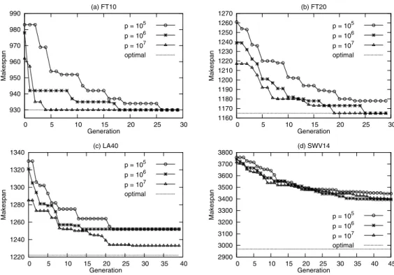
The results are shown in Figure 3. As the population size increases, fewer generations are required to converge.
930 940 950 960 970 980 990 0 5 10 15 20 25 30 Makespan Generation (a) FT10 p = 105 p = 106 p = 107 optimal 1160 1170 1180 1190 1200 1210 1220 1230 1240 1250 1260 1270 0 5 10 15 20 25 30 Makespan Generation (b) FT20 p = 105 p = 106 p = 107 optimal 1220 1240 1260 1280 1300 1320 1340 0 5 10 15 20 25 30 35 40 Makespan Generation (c) LA40 p = 105 p = 106 p = 107 optimal 2900 3000 3100 3200 3300 3400 3500 3600 3700 3800 0 5 10 15 20 25 30 35 40 45 Makespan Generation (d) SWV14 p = 105 p = 106 p = 107 optimal
Fig. 3. The results of GA with various population sizes𝑝for the problems (a) FT10, (b) FT20, (c) LA40, and (d) SWV14
Particularly in Figure 3(a), only 4 generations are required to reach the optimal makespan when𝑝= 107, while 18 and 26 generations are required when𝑝= 106and105, respectively. The same observation can be made in Figure 3(b), where 19 generations are required to reach the optimal makespan when 𝑝 = 107, while 25 are required by 𝑝 = 106. In Figure 3(c), although both experiments with𝑝= 105and106 converge at the same local minimum, the latter approaches it in fewer generations. Since MapReduce incurs overhead for every generation, it is desirable to find solutions with fewer generations. This can be achieved by using a larger population as shown in the results.
In addition, GAs with larger populations are more likely to find good solutions. In Figure 3(b), the experiment with𝑝= 105converges at a local minimum 1178, while the ones with
larger population sizes yield the optimal makespan of 1165. Similarly, in Figure 3(c), both experiments with𝑝= 105and 106converge at 1252, while a better makespan 1233 is found
by scaling the population size to107. In Figure 3(d), however, the effects of increasing population sizes are not phenomenal. The reason may be that this problem is too hard to be solved within a few tens of generations. More experiments with𝑝 > 107on a larger cluster must be performed to further investigate
this issue.
B. Effects of the Cluster Size
This experiment runs the GA on Amazon’s Elastic Compute Cloud (EC2) clusters of different sizes, and the completion time for each generation is observed. The GA is given a
50 100 150 200 250 300 350 400 0 2 4 6 8 10 12 14 16 18 20
Average runtime per generation (seconds) Machine instances
Fig. 4. The effects of cluster size
population of104individuals to solve LA40. For each cluster size, the GA is run for 10 generations, and the average execution times and the standard deviations are plotted in Figure 4. The execution time for a cluster of one machine is shown as a baseline for comparison with other clusters with multiple machines. As the number of machine instances in the cluster increases, the running time decreases as a result of increasing computing power. It is therefore beneficial to increase the cluster size when running GAs with large population sizes.
A typical profile of execution time for one generation is shown in Table II. The GA is given a population of size104 to solve LA40. Only 1 mapper and 1 reducer are used. The total job completion time and the cumulative running time
TABLE II
ATYPICAL PROFILE OF EXECUTION TIME WHEN RUNNING THEGAFOR ONE GENERATION TO SOLVELA40,USING ONE MAPPER AND ONE
REDUCER. THE POPULATION SIZE IS104. Job Completion Time map() reduce() Overhead
356.067 (seconds) 331.155 7.191 17.721
100% 93.00% 2.02% 4.98%
for the map and the reduce functions are recorded. Most of the execution time (i.e., ≈ 95%) is spent on running the
map and thereduce functions, while the remaining portion (≈ 5%) of the time is labeled as “overhead”. It is possible to reduce the observed overhead by introducing programming models that are optimized for iterative MapReduce jobs, such as Twister [22], which is one possible future direction.
IV. CONCLUSION
In this study, a GA for JSSP is implemented using Map-Reduce, and experiments are run with various population sizes (i.e., up to 107) and on clusters of various sizes. Our implementation of GA with MapReduce is based on [5], while adding more GA features to cope with real-world problems, including local search, non-random crossover, and non-random initial populations. The chromosome representation and the schedule evaluation for JSSP also increase the complexity.
The effects of large populations are prominent, in that a larger population tends not only to find a better solution, but also to converge with fewer generations. The results confirm what was mentioned in [23, p. 198-200], but our experiments consist of a much harder problem and much larger populations. Moreover, having fewer generations is beneficial due to the overall MapReduce overhead. Because for each MapReduce job there exists certain initialization/shuffling overhead, having fewer generations, and hence fewer iterations of MapReduce, reduces the overall overhead. The effects of cluster sizes is also presented, which show the speedup of execution time by increasing nodes in the cluster. This may serve as a rough guideline regarding what cluster size to use and what speedup to expect.
In general, GAs implemented with MapReduce provide new possibilities toward solving hard problems. To our knowledge, this is the first implementation with modern GA features that tackles real-world computationally intensive problems. The experiments with large populations also reveal interesting tradeoffs between population sizes and number of generations, whereby generations must be run sequentially, but larger populations allow us to arbitrarily parallelize.
ACKNOWLEDGMENTS
This work was supported in part by the NSF under awards IIS-0836560 and IIS-0916043, and also in part by Google and IBM, via the Academic Cloud Computing Initiative (ACCI). Any opinions, findings, conclusions, or recommendations ex-pressed are the authors’ and do not necessarily reflect those of the sponsors. The second author is grateful to Esther and Kiri for their loving support.
REFERENCES
[1] L. Davis et al., Handbook of genetic algorithms. Van Norstrand Reinhold, New York, 1991.
[2] E. Aarts and J. Korst,Simulated annealing and Boltzmann machines. John Wiley & Sons, New York, 1989.
[3] F. Glover and B. Meli´an, “Tabu search,”Metaheuristic Procedures for Training Neutral Networks, vol. 36, pp. 53–69, 2006.
[4] J. Dean and S. Ghemawat, “MapReduce: A flexible data processing tool,”Commun. ACM, vol. 53, no. 1, pp. 72–77, 2010.
[5] A. Verma, X. Llor`a, D. Goldberg, and R. Campbell, “Scaling genetic algorithms using MapReduce,”Proceedings of the 2009 Ninth Interna-tional Conference on Intelligent Systems Design and Applications, pp. 13–18, 2009.
[6] C. Jin, C. Vecchiola, and R. Buyya, “MRPGA: An extension of Map-Reduce for parallelizing genetic algorithms,”IEEE Fourth International Conference on eScience, 2008. eScience’08, pp. 214–221, 2008. [7] S. Reddi and C. Ramamoorthy, “On the flow-shop sequencing problem
with no wait in process,”Operational Research Quarterly, vol. 23, no. 3, pp. 323–331, 1972.
[8] S. Droste, T. Jansen, and I. Wegener, “Upper and lower bounds for randomized search heuristics in black-box optimization,” Theory of Computing Systems, vol. 39, no. 4, pp. 525–544, 2006.
[9] C. Witt, “Population size versus runtime of a simple evolutionary algorithm,”Theoretical Computer Science, vol. 403, no. 1, pp. 104–120, 2008.
[10] C. Bierwirth, D. Mattfeld, and H. Kopfer, “On permutation representa-tions for scheduling problems,”Parallel Problem Solving from Nature— PPSN IV, pp. 310–318, 1996.
[11] R. Cheng, M. Gen, and Y. Tsujimura, “A tutorial survey of job-shop scheduling problems using genetic algorithms–I. Representation,”
Computers and Industrial Engineering, vol. 30, no. 4, pp. 983–997, 1996.
[12] B. Giffler and G. Thompson, “Algorithms for solving production-scheduling problems,”Operations Research, vol. 8, no. 4, pp. 487–503, 1960.
[13] E. Nowicki and C. Smutnicki, “A fast taboo search algorithm for the job shop problem,”Management Science, vol. 42, no. 6, pp. 797–813, 1996.
[14] B. Park, H. Choi, and H. Kim, “A hybrid genetic algorithm for the job shop scheduling problems,”Computers & industrial engineering, vol. 45, no. 4, pp. 597–613, 2003.
[15] S. Luke and L. Spector, “A comparison of crossover and mutation in genetic programming,”Genetic Programming, vol. 97, pp. 240–248, 1997.
[16] J. Beasley, “OR-Library: Distributing test problems by electronic mail,”
Journal of the Operational Research Society, vol. 41, no. 11, pp. 1069– 1072, 1990.
[17] J. Muth and G. Thompson,Industrial scheduling. Prentice-Hall, 1963. [18] S. Lawrence, “Resource constrained project scheduling: An experimental investigation of heuristic scheduling techniques (Supplement),”Ph.D. Thesis Graduate School of Industrial Administration, Carnegie-Mellon University, Pittsburgh, PA, 1984.
[19] R. H. Storer, S. D. Wu, and R. Vaccari, “New search spaces for sequenc-ing problems with application to job shop schedulsequenc-ing,”Management Science, vol. 38, no. 10, pp. 1495–1509, October 1992.
[20] “http://www.google.com/intl/en/press/pressrel/ 20071008 ibm univ.html.”
[21] T. White,Hadoop: The Definitive Guide. O’Reilly Media, Inc., 2009. [22] J. Ekanayake, H. Li, B. Zhang, T. Gunarathne, S. Bae, J. Qiu, and G. Fox, “Twister: A runtime for iterative MapReduce,”Proceedings of the First International Workshop on MapReduce and its Applications (MAPREDUCE’10) of ACM HPDC2010, pp. 20–25, 2010.
[23] J. Koza,Genetic programming: On the programming of computers by means of natural selection. The MIT press, 1992.