For Peer Review Only
Estimating Value-at-Risk using a Multivariate Copula-Based Volatility Model.
Journal: The European Journal of Finance Manuscript ID REJF-2016-0199
Manuscript Type: Special Issue
Keywords: value-at-risk, dynamic conditional correlation, GARCH, volatility, copulas, risk management
For Peer Review Only
Abstract
This paper proposes a multivariate copula-based volatility model for estimating value-at-Risk in banks of some selected European countries by combining Dynamic Conditional Correla-tion (DCC) multivariate GARCH (M-GARCH) volatility model and copula funcCorrela-tions. Non-normality in multivariate models is associated with the joint probability of the univariate models’ marginal probabilities —the joint probability of large market movements, referred to as tail dependence. In this paper, we use copula functions to model the tail dependence of large market movements and test the validity of our results by performing back-testing tech-niques. The results show that the copula-based approach provides better estimates than the common methods currently used and captures VaR well based on the differences in the num-bers of exceptions produced during different observation periods at the same confidence level.
Keywords: value-at-risk, dynamic conditional correlation, GARCH, volatility, copulas, volatility, risk management.
J.E.L. classification: C15, C58, G11, G32. 2 3 4 5 6 7 8 9 10 11 12 13 14 15 16 17 18 19 20 21 22 23 24 25 26 27 28 29 30 31 32 33 34 35 36 37 38 39 40 41 42 43 44 45 46 47 48 49 50 51 52 53 54 55 56 57 58 59
For Peer Review Only
1
Introduction
Value-at-Risk (VaR) is a standard risk measure in financial risk management and is widely used in the banking sector and other financial institutions. It summarises the worst possible loss of a portfolio of financial assets at a given confidence level (CL) over a given time period. European banks began adopting VaR in the early 1990s. International bank regulators also influenced the development and use of VaR when the Basel Committee on Banking Supervision chose VaR as the international standard method for evaluating the market risk of a portfolio of financial assets for regulatory purposes (on Banking Supervision, 1996).
There are many methods to estimate VaR (see Holton (2014), Jorion (2007), Malz (2011) and the references therein), and the most common methods used by banks are the variance-covariance method (also known as the parametric or Delta Normal approach, was developed by J.P. Morgan using its RiskMetrics in 1993), historical simulation, and Monte Carlo sim-ulation. Due to their simplicity, variance-covariance methods appear to have been pervasive in the banking sector with over three-quarters of banks using them for calculating VaR (Drehmann, 2007). These methods are based on the assumption that the asset returns are independently and identically normally distributed, which of course, may not be the case in reality. This assumption contradicts empirical evidence, which shows that in many cases (for example see Sheikh and Qiao (2010)), financial asset returns are not independent and normally distributed —financial asset returns are, in fact, leptokurtic and fat-tailed, leading to underestimation or overestimation of VaR, as extremely large positive and negative asset returns are more likely in practice than normally distributed models predict.
Another drawback of these methods is in the estimation of the conditional volatility of financial returns. Most financial asset returns exhibit heavy tails (as explained earlier) with respect to conditional volatility over time. Berkowitz et al. (2011) also showed evidence of changing volatility and non-normality using desk-level data from a large international commercial bank. VaR models are highly dependent on the type of volatility model used. A good volatility model should be able to capture the behaviour of the tail distribution of asset
3 4 5 6 7 8 9 10 11 12 13 14 15 16 17 18 19 20 21 22 23 24 25 26 27 28 29 30 31 32 33 34 35 36 37 38 39 40 41 42 43 44 45 46 47 48 49 50 51 52 53 54 55 56 57 58
For Peer Review Only
returns, be easily implemented for a wide range of asset returns, and be easily extensible to portfolios with many risk factors of different kinds (Malz, 2011). For multivariate volatility models of VaR, we must focus on the tail dependence, which is the principal factor associated with non-normality.
Therefore, the purpose of this paper is to investigate the reliability of a VaR model constructed using a DCC M-GARCH volatility model and copulas.
The rest of the paper is structured as follows: Section 2 presents an overview of M-GARCH volatility models, the DCC model, and why they are important in VaR estimation. In Section 3, we introduce copulas (elliptical and Archimedean) and Sklar’s theorem. Section 4 presents invariant measures used in measuring the dependence structure. Section 5 presents empirical procedures and results of the VaR estimates. In Section 6, we discuss and present the results of back-testing techniques; this is followed by a summary and conclusion in Section 7.
2
Multivariate Volatility Models
Financial asset returns often demonstrate volatility clustering. Therefore, volatility plays an important role in VaR estimation. Many volatility models have been proposed, for example a generalised autoregressive conditional heteroskedasticity (GARCH) model and its exten-sion have been used to capture the effects of volatility clustering and asymmetry in VaR estimation. Numerous studies have applied a variety of univariate GARCH models in VaR estimation (see So and Philip (2006), Berkowitz and Obrien (2002), and McNeil and Frey (2000)). In addition, Kuester et al. (2006) provides an extensive review of VaR estimation methods with a focus on univariate GARCH models. The results of all these studies suggest that GARCH models provide more accurate VaR estimates than traditional methods.
Because financial applications typically deal with a portfolio of assets with several risk factors (as considered in this study), a multivariate GARCH model would be very useful for
2 3 4 5 6 7 8 9 10 11 12 13 14 15 16 17 18 19 20 21 22 23 24 25 26 27 28 29 30 31 32 33 34 35 36 37 38 39 40 41 42 43 44 45 46 47 48 49 50 51 52 53 54 55 56 57 58 59
For Peer Review Only
VaR estimation. Univariate VaR models focus on an individual portfolio, whereas the mul-tivariate approaches explicitly model the correlation structure of the covariance or volatility matrix of multiple asset returns over time.
Numerous multivariate GARCH models have since been developed (see Bollerslev et al. (1994), Engle and Kroner (1995), Fengler and Herwartz (2008), Tsay (2013) and the refer-ences therein). Bauwens et al. (2006) divides multivariate GARCH (M-GARCH) models into three categories: (i) direct generalisation of univariate GARCH models (e.g., exponentially-weighted moving average (EWMA), vector error correction (VEC), BEKK, etc.), (ii) lin-ear combinations of univariate GARCH models (e.g., generalised orthogonal GARCH (GO-GARCH), principal component GARCH (P(GO-GARCH), etc.), and (iii) nonlinear combinations of univariate GARCH models (e.g., dynamic conditional correlation (DCC) and constant conditional correlation (CCC)). Most volatility models fail to satisfy the positive definite conditions of the covariance matrix of asset returns. In this paper, we employ the DCC model in our analysis because of some conditions (to be discussed later) that will guarantee the conditional volatility matrix to be positive-definite almost surely. For more details on M-GARCH models, see (Silvennoinen and Ter¨asvirta, 2009) and (Ghalanos, 2015).
2.1
The DCC model
In the DCC model, the volatility matrix, Σt, consists of a marginal standardised vector of the series ηt, where ηt = σitait, and σit is the conditional volatility series obtained using GARCH(1,1) fori= 1, . . . , N. We can then represent the conditional volatility or covariance matrix as Σt =DtρtDt, (1) 3 4 5 6 7 8 9 10 11 12 13 14 15 16 17 18 19 20 21 22 23 24 25 26 27 28 29 30 31 32 33 34 35 36 37 38 39 40 41 42 43 44 45 46 47 48 49 50 51 52 53 54 55 56 57 58
For Peer Review Only
and the conditional correlation matrix is given by
ρt=Dt−1ΣtDt−1, (2)
whereDt is the diagonal matrix of thek conditional volatilities of the stock returns; that is,
D=diag√
σ11,t, . . . ,√σkk,t , and σij,tis the (i, j)th element of the volatility matrix (Tsay, 2005).
Tse and Tsui (2002) and Engle (2002) propose two types of DCC models. The DCC model of Tse and Tsui (DCCT(m)) is given by
ρt = (1−θ1−θ2) ¯ρt+θ1ρt−1+θ2ψt−1, (3)
whereθi ∈R+, 0 ≤θ1+θ2 <1 fori= 1,2. ¯ρtis akxkunconditional correlation matrix ofηt.
ψt−1 is a k x k correlation matrix of the most recent returns that depends on{ηt−1. . . ηt−m} and is defined as ψij,t−1 = Σm k=1ηi,t−kηj,t−k q (Σm k=1ηi,t−k2 )(Σmk=1ηj,t−k2 ) . (4)
If m > k, then ψt−1 and hence ρt are guaranteed to be positive-definite.
For the model proposed by Engle (DCCE(m)), the correlation matrix (Eq.(2)) depends on two parameters, θ1 and θ2, controlled by
Σt= (1−θ1−θ2) ¯Σt+θ1Σt−1+θ2ηt−1ηt−′ 1, (5)
and Σtis a positive-definite matrix. ¯Σtis the unconditional covariance matrix of ηt,θi ∈R+, 0< θ1+θ2 <1 for i= 1,2 (Tsay, 2013). 2 3 4 5 6 7 8 9 10 11 12 13 14 15 16 17 18 19 20 21 22 23 24 25 26 27 28 29 30 31 32 33 34 35 36 37 38 39 40 41 42 43 44 45 46 47 48 49 50 51 52 53 54 55 56 57 58 59
For Peer Review Only
3
Copulas
Non-normality in multivariate models is associated with the joint probability of the univariate models’ marginal probabilities, that is, the joint probability of large market movements referred to as tail dependence. The VaR estimation for a portfolio of assets can become very difficult due to the complexity of joint multivariate distributions. To overcome these problems, we use the copula theory, which enables us to construct a flexible multivariate distribution with different margins and different dependence structures; this allows the joint distribution of a portfolio to be free from assumptions of normality and linear correlation. Additionally, copulas can easily capture extreme dependencies such as tail dependence, while the normal distribution assumes no extreme dependencies.
The copula theory was first developed by Sklar (1959) and later introduced to the finance literature by Embrechts and McNeil (1999), Frey et al. (2001), and Li (1999). Consequently, Embrechts et al. (2002) introduced the application of copula theory to financial asset returns and Patton (2004) expanded the framework of the copula theory with respect to the time varying nature of financial dependence schemes. The copula theory has also been used in risk management to measure the VaR of portfolios, including both unconditional (Cherubini and Luciano (2001), Embrechts and Lindskog (2003), and Cherubini et al. (2004)) and, re-cently, conditional distributions (Silva Filho et al. (2014), Huang et al. (2009) and Fantazzini (2008)).
In this paper, we take advantage of copula theory and develop a copula-based volatility model.
For the purpose of estimating the VaR, we use the following version of Sklar’s theorem as given by Cherubini et al. (2004).
Theorem 1 Sklar’s theorem: Let F1(x1), . . . , Fn(xn) be known marginal distribution func-tions. Then, for every x= (x1, . . . , xn)∈ ℜ±n,
3 4 5 6 7 8 9 10 11 12 13 14 15 16 17 18 19 20 21 22 23 24 25 26 27 28 29 30 31 32 33 34 35 36 37 38 39 40 41 42 43 44 45 46 47 48 49 50 51 52 53 54 55 56 57 58
For Peer Review Only
• if c is any subcopula whose domain contains Ran F1× Ran F2×. . .× Ran Fn, then
c(F1(x1), F2(x2), . . . , Fn(xn))
is a joint distribution function with margins F1(x1), F2(x2), . . . , Fn(xn), and
• ifF is a joint distribution function with marginsF1(x1), F2(x2), . . . , Fn(xn), there exists a unique subcopula c, with domain Ran F1× Ran F2×. . .× Ran Fn, such that
F =c(F1(x1), F2(x2), . . . , Fn(xn)).
If F1(x1), F2(x2), . . . , Fn(xn) are continuous, the subcopula is a copula; if not, there exists a copula C such that
C(u1, u2, . . . , un) = c(u1, u2, . . . , un)
for every (u1, u2, . . . , un)∈ Ran F1× Ran F2×. . .× Ran Fn. Where ℜ±n= [−∞,+∞]n
and Ran F = range of the function F.
Definition 1 An n−dimensional copula C(u1, u2, u3, . . . , un)
′
is a distribution function on In with standard uniform marginal distributions (Tsay, 2013).
Consider a random vector X = (x1, . . . , xn)
′
, with margins F(x1), . . . , F(xn); then, from Theorem 1,
F(x1, . . . , xn) = C(F(x1), . . . , F(xn)). (6)
C is unique if F(x1), . . . , F(xn) are continuous; otherwise, C is uniquely determined onIn (I = [0,1]; a unit interval on the real line.). On the other hand, ifC is a copula andF1, . . . , Fn are univariate distribution functions, Eq.(6) is a joint distribution function with margins
F1, . . . , Fn (Ghalanos, 2015), (Tsay, 2013). 2 3 4 5 6 7 8 9 10 11 12 13 14 15 16 17 18 19 20 21 22 23 24 25 26 27 28 29 30 31 32 33 34 35 36 37 38 39 40 41 42 43 44 45 46 47 48 49 50 51 52 53 54 55 56 57 58 59
For Peer Review Only
Definition 2 Each copula C(u1, . . . , un) has a densityc(u1, . . . , un)related to it and defined as
c(u1, . . . , un) =
∂nC(u1, . . . , un)
∂u1, . . . , ∂un
, (7)
and the density function for the copula is
f(x1, . . . , xn) =c(F1(x1, . . . , Fn(xn)) n
Y
i=1
fi(xi) (8)
in In for a continuous random variable, where fi are the marginal densities (Cherubini et al., 2004), (Ghalanos, 2015).
Bob (2013) and Cherubini et al. (2011) discuss two commonly used families of copulas in financial applications: the elliptical and the Archimedean copulas.
3.1
Elliptical Copulas
The most common elliptical copulas are the Gaussian and the Student’s t copulas, which are symmetric. The dependence structure is determined by the standardised correlation or dispersion matrix R = 1 . . . ρ1,n ... ... ... ρn,1 . . . 1 (9)
because of the invariant property of copulas. ρi,j is the dispersion parameter, which can be set to either Kendall’s tau or Spearman’s rho, as discussed later.
3 4 5 6 7 8 9 10 11 12 13 14 15 16 17 18 19 20 21 22 23 24 25 26 27 28 29 30 31 32 33 34 35 36 37 38 39 40 41 42 43 44 45 46 47 48 49 50 51 52 53 54 55 56 57 58
For Peer Review Only
Consider a symmetric positive definite matrix (Eq.9) with diag(R) = (1,1, . . . ,1)T; we can represent the multivariate Gaussian copula (MGC) as
CRGa =P(Φ(X1)≤u1, . . . ,Φ(Xn)≤un) = ΦR(Φ−1(u1), . . . ,Φ−1(un)), (10)
where ΦRis the standardised multivariate normal distribution and Φ−R1is the inverse standard univariate normal distribution function of u with correlation matrix R. If the margins are normal, then the Gaussian copula will generate the standard Gaussian joint distribution function with density function
cGaR (u1, u2, . . . , un) = 1 |R|12 exp −12ςT(R−1−I)ς , (11) where ς = (Φ−1(u 1), . . . ,Φ−1(un))T.
On the other hand, the multivariate Student’st copula (MTC) can be represented as
TR,v(u1, . . . , un) = tR,v(t−v1(u1), . . . , t −1
v (un)) (12)
with density function
cR,v(u1, . . . , un) = |R|− 1 2Γ( v+n 2 ) Γ(v2) Γ(v 2) Γ(v+1 2 ) n(1 + 1 vς TR−1ς)−v+2n Qn j=1 1 + ς 2 j v −v+12 , (13)
where tR,v is the standardised Student’s t distribution with correlation matrix R and v degrees of freedom. 2 3 4 5 6 7 8 9 10 11 12 13 14 15 16 17 18 19 20 21 22 23 24 25 26 27 28 29 30 31 32 33 34 35 36 37 38 39 40 41 42 43 44 45 46 47 48 49 50 51 52 53 54 55 56 57 58 59
For Peer Review Only
3.2
Archimedean Copulas:
Archimedean copulas are built via a generator as
C(u1, . . . , un) =ϕ−1(ϕ(u1) +. . .+ϕ(un)) (14)
with density function
c(u1, . . . , un) = ϕ−1(ϕ(u1) +. . .+ϕ(un)) n
Y
i=1
ϕ′(ui), (15)
whereϕ is the copula generator andϕ−1 is completely monotonic on [0,∞]. That is, ϕmust be infinitely differentiable with derivatives of ascending order and alternative sign such that
ϕ−1(0) = 1 and lim
x→+∞ϕ(x) = 0 (Cherubini et al., 2011). Thus, ϕ
′
(u) < 0 (i.e., ϕ is strictly decreasing) and ϕ′′
(u)>0 (i.e.,ϕ is strictly convex).
Archimedean copulas are very useful in risk management analysis because they capture an asymmetric tail dependence between financial asset returns. The most common are Gumbel (1960), Clayton (1978) and Frank (1979) copulas (Yan et al., 2007).
The Gumbel copula captures upper tail dependence, is limited to positive dependence, and has generator function ϕ(u) = (−ln(u))α and generator inverse ϕ−1(x) = exp(−x1
α). This will generate a Gumbel n-copula represented by
C(u1, . . . , un) = exp − " n X i=1 (−lnui)δ #1δ δ >0. (16) 3 4 5 6 7 8 9 10 11 12 13 14 15 16 17 18 19 20 21 22 23 24 25 26 27 28 29 30 31 32 33 34 35 36 37 38 39 40 41 42 43 44 45 46 47 48 49 50 51 52 53 54 55 56 57 58
For Peer Review Only
The generator function for the Clayton copula is given by ϕ(u) =u−α−1 and generator inverse ϕ−1(x) = (x+ 1)−1α, which yields a Clayton n-copula represented by
C(u1, . . . , un) = " n X i=1 (u−αi −n+ 1 #−α1 α >0. (17)
The Frank copula has generator function ϕ(u) = lnexp(exp(−−ααu))−−11 and generator inverse
ϕ−1(x) =
−α1 ln (1 +e x(e−α
−1)), which will result in a Frank n-copula represented by
C(u1, . . . , un) = − 1 αln 1 + Qn i=1(e−αui −1) (e−α−1)n−1 α=>0, (18) (Cherubini et al., 2004).
4
Measuring Dependence
The traditional way to measure the relationship between markets and risk factors is by looking at their linear correlations, which depend both on the marginal and joint distributions of the risk factors. If there is no linear relationship —in the case of non-normality —the results might be misleading (see Cherubini et al. (2011)). In this situation, nonparametric invariant measures that are not dependent on marginal probability distributions are more appropriate. Copulas measure a form of dependence between pairs of risk factors (i.e., asset returns) known as concordance using invariant measures.
Two observations (xi, yi) and (xj, yj) from a vector (X, Y) of continuous random variables are concordant if (xi−xj)(yi−yj)>0 and discordant if (xi−xj)(yi−yj)<0. Large values of X are paired with large values of Y and small values of X are paired with small values of Y as the proportion of concordant pairs in the sample increases. On the other hand, the proportion of concordant pairs decreases as large values of X are paired with small values of Y and small values ofX are paired with large values of Y (Alexander, 2008).
The most commonly used invariant measures are Kendall’s tau and Spearman’s rho.
2 3 4 5 6 7 8 9 10 11 12 13 14 15 16 17 18 19 20 21 22 23 24 25 26 27 28 29 30 31 32 33 34 35 36 37 38 39 40 41 42 43 44 45 46 47 48 49 50 51 52 53 54 55 56 57 58 59
For Peer Review Only
Consider n paired continuous observations (xi, yi) ranked from smallest to largest, with the smallest ranked 1, the second smallest ranked 2 and so on. Then, Kendall’s tau is defined as the sum of the number of concordant pairs minus the sum of the number of discordant pairs divided by the total number of pairs, i.e., the probability of concordance minus the probability of discordance:
τX,Y =P[(xi−xj)(yi−yj)>0]−P[(xi−xj)(yi−yj)<0] =
C−D
C+D, (19)
where C is the number of concordant pairs below a particular rank that are larger in value than that particular rank, and D is the number of discordant pairs below a particular rank that are smaller in value than that particular rank.
Spearman’s rho, on the other hand, is defined as the probability of concordance minus the probability of discordance of the pair of vectors (x1, y1) and (x2, y3) with the same margins. That is,
ρX,Y = 3(P[(x1−x2)(y1−y3)>0]−P[(x1−x2)(y1−y3)]<0).
The joint distribution function of (x1, y1) is H(x, y), while the joint distribution function of (x2, y3) is F(x), G(y) because x2 and y3 are independent (Nelsen, 2007). Alternatively,
ρX,Y = 1− 6Pn
i=1d2i
n(n2−1), where d is the difference between the ranked samples.
Nelsen (2007) has shown that Kendall’s tau and Spearman’s rho depend on the vectors (x1, y1), (x2, y2) and (x1, y1), (x2, y3), respectively, through theirs copulas C, and that the following relationship holds:
τX,Y = 4 Z 1 0 Z 1 0 C(u, v)dC(u, v)−1 3 4 5 6 7 8 9 10 11 12 13 14 15 16 17 18 19 20 21 22 23 24 25 26 27 28 29 30 31 32 33 34 35 36 37 38 39 40 41 42 43 44 45 46 47 48 49 50 51 52 53 54 55 56 57 58
For Peer Review Only
ρX,Y = 12 Z 1 0 Z 1 0 C(u, v)dudv−3.5
Empirical Analysis
5.1
Data
We investigate the performance of an M-GARCH DCC copula-based volatility model in VaR estimation using daily closing stock prices of 47 banking sector stocks from seven different EU countries —Germany, the UK, Sweden, France, Italy, Spain, and Greece —over the period from 31 December 2004 to 31 December 2015. All data are from DataStream and consist of 2870 observations.
The daily log return series of the stocks are calculated via
rt = log S1,t+τ S1,t , . . . , log SN,t+τ SN,t = (r1t, . . . , rN t), (20)
where N represents the number of stocks in the sample. Figures 1 to 7 shows time series plots of daily log returns series for the different countries. From the plots, we can observe the presence of volatility clustering. That is, small changes in volatility tend to be followed by small changes for a prolonged period of time and large changes in volatility tend to be followed by large changes for a prolonged period of time. Basic statistics of the stock returns are reported in percentages in Table 1. From the table, we see that the stock returns are far from being normally distributed, as indicated by their high excess kurtosis and skewness. We confirm this by running a multivariate ARCH test, as described by Tsay (2013), on the log returns at 5% significance. The results confirm the presence of conditional heteroskedasticity in the daily log return series with a P −value equal to or close to zero.
2 3 4 5 6 7 8 9 10 11 12 13 14 15 16 17 18 19 20 21 22 23 24 25 26 27 28 29 30 31 32 33 34 35 36 37 38 39 40 41 42 43 44 45 46 47 48 49 50 51 52 53 54 55 56 57 58 59
For Peer Review Only
Country Stocks
France F.BNP F.SGE F.CRDA F.KNF F.CC F.CAI F.CAMO F.LAV F.CAIV F.CPD Mean 0.0006 -0.0151 -0.0215 -0.0019 0.0006 -0.0108 -0.0102 -0.0011 -0.0103 -0.0166 Variance 0.0647 0.0807 0.0764 0.0959 0.0197 0.0145 0.0262 0.0267 0.0225 0.0202 Stdev 2.5427 2.8399 2.7645 3.0969 1.4027 1.2029 1.6182 1.6340 1.5003 1.4212 Skewness 34.4305 6.9738 27.7890 60.0710 62.1017 7.6754 -43.2826 -46.9617 5.3467 -1.5654 Excess Kurtosis 867.8928 680.0429 624.0289 1209.1365 821.6399 678.3979 476.7556 1107.4525 601.0420 702.8488 Italy I.ISP I.UCG I.MB I.PMI I.BMPS I.BP I.UBI I.BPE I.CE I.BPSO
Mean -0.0023 -0.0519 -0.0078 -0.0250 -0.1260 -0.0635 -0.0278 -0.0129 -0.0022 -0.0132 Variance 0.0671 0.0829 0.0429 0.0773 0.0870 0.0814 0.0566 0.0574 0.0517 0.0335 Stdev 2.5905 2.8797 2.0722 2.7800 2.9488 2.8539 2.3799 2.3966 2.2734 1.8305 Skewness -25.1383 -16.0663 3.8658 29.6811 -24.7777 2.9842 -4.4575 24.7941 1.4148 58.9718 Excess Kurtosis 656.5973 589.0746 320.6962 383.9322 891.5712 461.0507 273.2804 392.4517 408.2981 553.0105 UK HSBA BARC LLOY RBS STAN CIHL
Mean -0.0124 -0.0306 -0.0407 -0.0971 -0.0112 -0.1171 Variance 0.0293 0.1030 0.1077 0.1504 0.0594 0.0762 Stdev 1.7122 3.2098 3.2823 3.8785 2.4376 2.7600 Skewness -33.6697 143.8658 -105.4936 -840.1325 31.6077 9.0031 Excess Kurtosis 1690.7965 4021.7880 3727.5413 23552.6326 1308.5010 4940.1441 Germany D.DBK D.CBK D.IKB D.MBK D.OLB D.UBK
Mean -0.0320 -0.0782 -0.1287 0.0008 -0.0457 0.0879 Variance 0.0615 0.0904 0.1529 0.0550 0.0478 0.0466 Stdev 2.4803 3.0066 3.9100 2.3445 2.1863 2.1586 Skewness 32.5034 -13.9034 151.9830 31.5160 83.5634 -31.7385 Excess Kurtosis 1022.5506 873.5286 1914.4094 1145.6160 2008.7958 1984.3534 Greece G.PIST G.PEIR G.EFG G.ETE G.ATT G.ELL
Mean -0.1603 -0.3371 -0.3377 -0.2872 -0.2045 -0.0642 Variance 0.2287 0.2876 0.3162 0.2487 0.2818 0.0448 Stdev 4.7826 5.3624 5.6234 4.9866 5.3087 2.1157 Skewness -12.5182 -105.8321 -61.0233 -103.6301 -59.4886 -7.5496 Excess Kurtosis 827.1241 1063.2666 865.8341 1044.0274 1317.2709 1519.9341 Spain E.SCH E.BBVA E.BSAB E.BKT E.POP
Mean -0.0070 -0.0154 -0.0199 0.0117 -0.0702 Variance 0.0463 0.0444 0.0359 0.0512 0.0529 Stdev 2.1519 2.1078 1.8940 2.2617 2.2991 Skewness 20.4736 32.7311 71.6545 49.2691 43.5654 Excess Kurtosis 828.4460 668.4718 623.2511 304.9592 494.7029 Sweden W.NDA W.SVK W.SWED W.SEA
Mean 0.0202 0.0234 0.0109 0.0104 Variance 0.0419 0.0347 0.0631 0.0643 Stdev 2.0471 1.8633 2.5116 2.5361 Skewness 52.6835 12.2476 -20.9301 5.3782 Excess Kurtosis 657.9097 690.7580 906.9637 1278.0779
Table 1: Basic statistics of stock returns (in percentages). High excess kurtosis and skewness implies stock returns are not normally distributed. 13 URL: http://mc.manuscriptcentral.com/rejf 3 4 5 6 7 8 9 10 11 12 13 14 15 16 17 18 19 20 21 22 23 24 25 26 27 28 29 30 31 32 33 34 35 36 37 38 39 40 41 42 43 44 45 46 47 48 49 50 51 52 53 54 55 56
For Peer Review Only
5.2
Modelling the volatility matrix and copula parameters
We obtained the volatility matrix P
t, which consists of the marginal standardised residu-als {ηi,t}Tt=1, by applying the M-GARCH DCC model to the log return series and setting the conditional distribution of the standardised residuals to the Student’s t distribution to account for the heavy tails.
Copula parameters are estimated by the canonical maximum likelihood (CML) method (Cherubini et al., 2004). That is, we use pseudo-observations of the standardised residuals to estimate the marginals and then estimated the copula parameters by means of maximum likelihood estimation (MLE):
ˆ θ2 =ArgM axθ2 T X t=1 lnc( ˆF1(x1t), . . . ,Fˆn(xnt);θ2). (21)
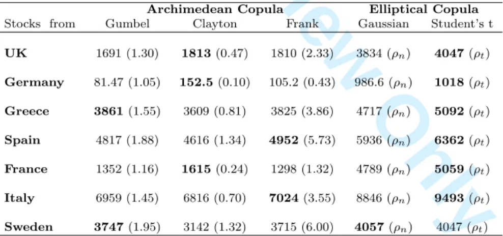
The best copula to use for our VaR modelling is selected by comparing MLE values. We select two models, one from each copula family. Table 2 shows the MLEs and copula parameter values for both Archimedean and elliptical copulas.
Stocks from
Archimedean Copula Elliptical Copula
Gumbel Clayton Frank Gaussian Student’s t
UK 1691 (1.30) 1813(0.47) 1810 (2.33) 3834 (ρn) 4047(ρt) Germany 81.47 (1.05) 152.5(0.10) 105.2 (0.43) 986.6 (ρn) 1018(ρt) Greece 3861(1.55) 3609 (0.81) 3825 (3.86) 4717 (ρn) 5092(ρt) Spain 4817 (1.88) 4616 (1.34) 4952(5.73) 5936 (ρn) 6362(ρt) France 1352 (1.16) 1615(0.24) 1298 (1.32) 4789 (ρn) 5059(ρt) Italy 6959 (1.45) 6816 (0.70) 7024(3.55) 8846 (ρn) 9493(ρt) Sweden 3747(1.95) 3142 (1.32) 3715 (6.00) 4057(ρn) 4047 (ρt)
Table 2: MLE and copula parameter (in parentheses) values. The best copula that fits the data (in bold) is selected based on the highest MLE value.
2 3 4 5 6 7 8 9 10 11 12 13 14 15 16 17 18 19 20 21 22 23 24 25 26 27 28 29 30 31 32 33 34 35 36 37 38 39 40 41 42 43 44 45 46 47 48 49 50 51 52 53 54 55 56 57 58 59
For Peer Review Only
5.3
Modelling the marginal distributions
Next, we specify the desired marginal distributions, which we set to a Student’stdistribution, and generate 10000 simulations from the fitted copula. Our choice of Student’stdistributions for the margins is because a multivariate ARCH test on the standardised residuals {ηi,t}Tt=1 still indicates the presence of volatility clustering. We then reintroduce the GARCH(1,1) model and convert the daily simulated data with t-margins to daily risk factor returns.That is,
xi,t =µi+ ˆσi,tζi,t , and
ˆ
σt2 =α0+α1ξt−2 1+β1σt−2 1, (22)
where i = 1, . . . n represents the stocks in each country, t = 1. . . T represents the length of the original data = 2869, andζi,t are the daily simulated observations from the copulas with
t-margins. α0, α1, and β1 are the GARCH parameters, µi are the unconditional means of the risk factors, and ˆσi are estimates of the conditional volatilities of the risk factors from the M-GARCH DCC model.
5.4
Estimating VaRs
For each country, we apply the risk factor mappings to construct a simulated portfolio of returns consisting of all stocks represented by
¯ Rp,t=E(Rp,t) = N X t=1 wiE(Ri,t), (23) where wi = Pn j=1xij PN j=1Cj , and N X i=1 wi = 1 1≤i≤n, 1≤j ≤N. 3 4 5 6 7 8 9 10 11 12 13 14 15 16 17 18 19 20 21 22 23 24 25 26 27 28 29 30 31 32 33 34 35 36 37 38 39 40 41 42 43 44 45 46 47 48 49 50 51 52 53 54 55 56 57 58
For Peer Review Only
¯
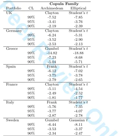
Rp,t is the expected return of the portfolio at timet; xij is the amount invested in asseti;Cj is the total dollar amount invested; andwi the weight of asset i. We assume equal weights. The one day VaR at timet withα% confidence level is simply the 1−α percentile of the distribution of the simulated portfolio returns below which lies (1−α)% of the observations and above which lies α% of the observations. Thus, we are α% confident that in the worst case scenario, the losses on the portfolio will not exceed the 1−αquantile. Table 3 shows VaR estimates with confidence levelsα= 99%,95%, and 90%, based on the selected Archimedean and elliptical copulas for the constructed portfolios.
Copula Family
Portfolio CL Archimedean Elliptical
UK Clayton Student’st
99% -7.52 -7.85
95% -3.41 -3.76
90% -2.19 -2.39
Germany Clayton Student’st
99% -6.24 -5.31
95% -3.52 -2.90
90% -2.53 -2.13
Greece Gumbel Student’st 99% -14.82 -18.88
95% -7.23 -8.68
90% -5.04 -5.71
Spain Frank Student’st
99% -6.12 -7.02
95% -3.75 -3.78
90% -2.79 -2.65
France Clayton Student’st
99% -5.11 -4.54
95% -2.49 -2.52
90% -1.81 -1.77
Italy Frank Student’st
99% -5.76 -7.35
95% -3.77 -4.07
90% -2.87 -2.78
Sweden Gumbel Gaussiant
99% -6.44 -8.11
95% -3.53 -3.37
90% -2.34 -2.47
Table 3: VaR estimates (in percentages) for the portfolio constructed from returns generated using Archimedean and elliptical copulas.
6
Back-testing
To check that the model does not overestimate or underestimate risk, we do back-testing on the model. This involves comparing the estimated VaRs for a given number of days T to
2 3 4 5 6 7 8 9 10 11 12 13 14 15 16 17 18 19 20 21 22 23 24 25 26 27 28 29 30 31 32 33 34 35 36 37 38 39 40 41 42 43 44 45 46 47 48 49 50 51 52 53 54 55 56 57 58 59
For Peer Review Only
the subsequent portfolio returns. The number of days N in which the loss on the portfolio exceeds VaR is recorded as the number of exceptions or failures. Too many exceptions implies the VaR model underestimates the level of risk on the portfolio, and too few exceptions implies the model overestimates risk. The number of exceptions should be reasonably close to T(1−c)% (c = confidence level), depends on the choice of c, and follows a binomial distribution
f(x) = Tx
pxqT−x (24)
with mean =pT and variance =pqT; q = 1−p and p= 1−c(Best, 2000).
6.1
Back-testing methods
The most popular back-testing methods include the standard normal hypothesis (or failure rate) test , Kupiec’s (1995) “proportion of failures” (POF) test, Basel’s (1996a) “traffic light” test, and Christoffersen’s (1998) test. We employ the standard normal hypothesis test, Basel’s “traffic light” test, and Kupiec’s POF test to check the reliability of the VaR models.
6.2
Standard normal hypothesis test
From the central limit theorem and with sufficiently large T, Eq.(24) can be approximated by the normal distribution
z = x√−pT
pqT ≈N(0,1), (25)
which is also the test statistic for a standard normal hypothesis test to assess the reliability of the VaR model (Jorion, 2007). The VaR model is rejected if z < −zα/2 or z > zα/2 for a two-tailed test and if z > zα for a one-tailed test. α= 1−c, and zα/2 and zα are the cutoff
3 4 5 6 7 8 9 10 11 12 13 14 15 16 17 18 19 20 21 22 23 24 25 26 27 28 29 30 31 32 33 34 35 36 37 38 39 40 41 42 43 44 45 46 47 48 49 50 51 52 53 54 55 56 57 58
For Peer Review Only
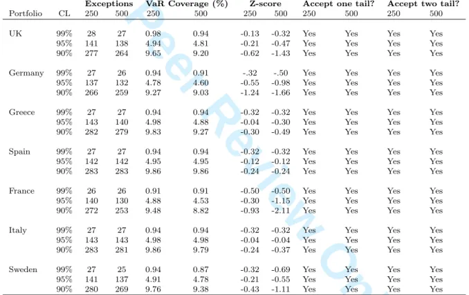
values for the inverse standard normal cumulative distribution of α and α/2, respectively. Tables 5 and 6 show back-testing results based on the standard normal hypothesis test.
6.3
Basel “traffic light” test
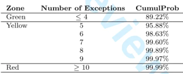
The Basel “traffic light” approach to back-testing the VaR was originally proposed by the Basel Committee of Banking and Supervision (BCBS) and is described in (on Banking Su-pervision, 1996). In a new accord, the BCBS further came up with a set of requirements that the VaR model must satisfy for it to be considered a reliable risk measure (Resti, 2008). That is, (i) VaR must be calculated with 99% confidence, (ii) back-testing must be done using a minimum of a one year observation period and must be tested over at least 250 days, (iii) regulators should be 95% confident that they are not erroneously rejecting a valid VaR model, and (iv) Basel specifies a one-tailed test —it is only interested in the underestimation of risk. Table 4 shows the acceptance region for the Basel “traffic light” approach.
Zone Number of Exceptions CumulProb
Green ≤4 89.22% Yellow 5 95.88% 6 98.63% 7 99.60% 8 99.89% 9 99.97% Red ≥10 99.99%
Table 4: Acceptance region for Basel “traffic light” approach for back-testing VaR models.
CL= 99%,T = 250 (Jorion, 2007).
Depending on the number of exceptions, the bank is placed in a red, green or yellow zone. Test results based on this test are shown in Table 7
6.4
Kupiec’s POF test
Kupiec defined an approximate 95% confidence region whereby the number of exceptions produced by the model must be within this interval for it to be considered a reliable risk measure. The confidence region is approximated using a chi-square distribution with one
2 3 4 5 6 7 8 9 10 11 12 13 14 15 16 17 18 19 20 21 22 23 24 25 26 27 28 29 30 31 32 33 34 35 36 37 38 39 40 41 42 43 44 45 46 47 48 49 50 51 52 53 54 55 56 57 58 59
For Peer Review Only
degree of freedom, defined as
LRP F = 2ln " 1− NTT−N N T N qT−NpN # . (26)
Assuming one degree of freedom and at a 5% confidence level, the chi-square value is 3.841. Hence, by equating Eq.(26) to 3.841 and solving for N, we obtain two values of N; the rejection region is [x1, x2]. The VaR model is rejected if N /∈ [x1, x2] and accepted if N ∈ [x1, x2] (Holton, 2002). Results based on this test are shown in Tables 8 and 9.
Exceptions VaR Coverage (%) Z-score Accept one tail? Accept two tail?
Portfolio CL 250 500 250 500 250 500 250 500 250 500
UK 99% 28 27 0.98 0.94 -0.13 -0.32 Yes Yes Yes Yes
95% 141 138 4.94 4.81 -0.21 -0.47 Yes Yes Yes Yes
90% 277 264 9.65 9.20 -0.62 -1.43 Yes Yes Yes Yes
Germany 99% 27 26 0.94 0.91 -.32 -.50 Yes Yes Yes Yes
95% 137 132 4.78 4.60 -0.55 -0.98 Yes Yes Yes Yes
90% 266 259 9.27 9.03 -1.24 -1.66 Yes Yes Yes Yes
Greece 99% 27 27 0.94 0.94 -0.32 -0.32 Yes Yes Yes Yes
95% 143 140 4.98 4.88 -0.04 -0.30 Yes Yes Yes Yes
90% 282 279 9.83 9.27 -0.30 -0.49 Yes Yes Yes Yes
Spain 99% 27 27 0.94 0.94 -0.32 -0.32 Yes Yes Yes Yes
95% 142 142 4.95 4.95 -0.12 -0.12 Yes Yes Yes Yes
90% 283 283 9.86 9.86 -0.24 -0.24 Yes Yes Yes Yes
France 99% 26 26 0.91 0.91 -0.50 -0.50 Yes Yes Yes Yes
95% 140 130 4.88 4.53 -0.30 -1.15 Yes Yes Yes Yes
90% 272 253 9.48 8.82 -0.93 -2.11 Yes Yes Yes Yes
Italy 99% 27 27 0.94 0.94 -0.32 -0.32 Yes Yes Yes Yes
95% 143 143 4.98 4.98 -0.04 -0.04 Yes Yes Yes Yes
90% 283 281 9.86 9.79 -0.24 -0.37 Yes Yes Yes Yes
Sweden 99% 27 25 0.94 0.87 -0.32 -0.69 Yes Yes Yes Yes
95% 141 137 4.91 4.78 -0.21 -0.55 Yes Yes Yes Yes
90% 280 269 9.76 9.38 -0.43 -1.11 Yes Yes Yes Yes
Table 5: Testing the reliability of the VaR model based on a standard normal hypothesis test. Returns generated using selected Archimedean copulas; time horizon = 1 day, 250-day and 500-day observation periods.
3 4 5 6 7 8 9 10 11 12 13 14 15 16 17 18 19 20 21 22 23 24 25 26 27 28 29 30 31 32 33 34 35 36 37 38 39 40 41 42 43 44 45 46 47 48 49 50 51 52 53 54 55 56 57 58
For Peer Review Only
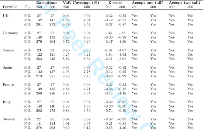
Exceptions VaR Coverage (%) Z-score Accept one tail? Accept two tail?
Portfolio CL 250 500 250 500 250 500 250 500 250 500
UK 99% 27 27 0.94 0.94 -0.32 -0.32 Yes Yes Yes Yes
95% 142 141 4.95 4.91 -0.12 -0.21 Yes Yes Yes Yes
90% 281 273 9.79 9.52 -0.37 -0.87 Yes Yes Yes Yes
Germany 99% 27 27 0.94 0.94 -.32 -.32 Yes Yes Yes Yes
95% 140 132 4.88 4.60 -0.30 -0.98 Yes Yes Yes Yes
90% 279 264 9.72 9.20 -0.47 -1.36 Yes Yes Yes Yes
Greece 99% 23 23 0.80 0.80 -1.07 -1.07 Yes Yes Yes Yes
95% 122 121 4.25 4.22 -1.84 -1.92 Yes Yes Yes Yes
90% 253 245 8.82 8.54 -2.11 -2.61 Yes Yes Yes Yes
Spain 99% 27 27 0.94 0.94 -0.32 -0.32 Yes Yes Yes Yes
95% 142 137 4.95 7.78 -0.12 -0.55 Yes Yes Yes Yes
90% 279 271 9.72 9.45 -0.49 -0.99 Yes Yes Yes Yes
France 99% 27 27 0.94 0.94 -0.32 -0.32 Yes Yes Yes Yes
95% 139 135 4.84 4.71 -0.38 -0.72 Yes Yes Yes Yes
90% 280 286 9.76 9.34 -0.43 -1.18 Yes Yes Yes Yes
Italy 99% 27 27 0.94 0.94 -0.32 -0.32 Yes Yes Yes Yes
95% 140 140 4.88 4.88 -0.30 -0.30 Yes Yes Yes Yes
90% 282 275 9.83 9.59 -0.74 -0.30 Yes Yes Yes Yes
Sweden 99% 27 25 0.94 0.87 -0.32 -0.69 Yes Yes Yes Yes
95% 141 134 4.91 4.67 -0.21 -0.81 Yes Yes Yes Yes
90% 278 263 9.69 9.17 -0.55 -1.49 Yes Yes Yes Yes
Table 6: Testing the reliability of the VaR model based on standard normal hypothesis test. Returns generated using selected elliptical copulas; time horizon = 1 day; 250-day and 500-day observation periods.
2 3 4 5 6 7 8 9 10 11 12 13 14 15 16 17 18 19 20 21 22 23 24 25 26 27 28 29 30 31 32 33 34 35 36 37 38 39 40 41 42 43 44 45 46 47 48 49 50 51 52 53 54 55 56 57 58 59
For Peer Review Only
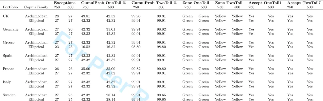
Exceptions CumulProb OneTail% CumulProb TwoTail% Zone OneTail Zone TwoTail Accept OneTail? Accept TwoTail?
Portfolio CopulaFamily 250 500 250 500 250 500 250 500 250 500 250 500 250 500 UK Archimedean 28 27 49.81 42.32 99.96 99.91 Green Green Yellow Yellow Yes Yes Yes Yes Elliptical 27 27 42.32 42.32 99.91 99.91 Green Green Yellow Yellow Yes Yes Yes Yes Germany Archimedean 27 26 42.32 35.01 99.91 98.82 Green Green Yellow Yellow Yes Yes Yes Yes Elliptical 27 27 42.32 42.32 99.91 99.91 Green Green Yellow Yellow Yes Yes Yes Yes Greece Archimedean 27 27 42.32 42.32 99.91 99.91 Green Green Yellow Yellow Yes Yes Yes Yes Elliptical 23 23 16.52 16.52 98.80 98.80 Green Green Yellow Yellow Yes Yes Yes Yes Spain Archimedean 27 27 42.32 42.32 99.91 99.91 Green Green Yellow Yellow Yes Yes Yes Yes Elliptical 27 27 42.32 42.32 99.91 99.91 Green Green Yellow Yellow Yes Yes Yes Yes France Archimedean 26 26 35.00 35.00 99.82 99.82 Green Green Yellow Yellow Yes Yes Yes Yes Elliptical 27 27 42.32 42.32 99.91 99.91 Green Green Yellow Yellow Yes Yes Yes Yes Italy Archimedean 27 27 42.32 42.32 99.91 99.91 Green Green Yellow Yellow Yes Yes Yes Yes Elliptical 27 27 42.32 42.32 99.91 99.91 Green Green Yellow Yellow Yes Yes Yes Yes Sweden Archimedean 27 25 42.32 28.14 99.91 99.65 Green Green Yellow Yellow Yes Yes Yes Yes Elliptical 27 25 42.32 28.14 99.91 99.65 Green Green Yellow Yellow Yes Yes Yes Yes
Table 7: Testing the reliability of the VaR model based on BCBS requirements. Time horizon = 1 day; 250- and 500-day observation periods. CumulProb = cumulative probability.
21 URL: http://mc.manuscriptcentral.com/rejf 3 4 5 6 7 8 9 10 11 12 13 14 15 16 17 18 19 20 21 22 23 24 25 26 27 28 29 30 31 32 33 34 35 36 37 38 39 40 41 42 43 44 45 46 47 48 49 50 51 52 53 54 55 56
For Peer Review Only
Exceptions Test Statistic Accept?
Portfolio CL 250 500 250 500 250 500
UK 99% 28 27 0.02 0.10 Yes Yes
95% 141 138 0.04 0.22 Yes Yes
90% 277 264 NaN NaN No No
Germany 99% 27 26 0.10 0.26 Yes Yes 95% 137 132 0.31 0.99 Yes Yes
90% 266 259 NaN NaN No No
Greece 99% 27 27 0.1 0.1 Yes Yes 95% 143 140 0.00 0.09 Yes No
90% 282 279 NaN NaN No No
Spain 99% 27 27 0.10 0.10 Yes Yes 95% 142 142 0.02 0.02 Yes Yes
90% 283 283 NaN NaN No No
France 99% 26 26 0.26 0.26 Yes Yes 95% 140 130 0.09 1.37 Yes Yes
90% 272 253 NaN NaN No No
Italy 99% 27 27 0.10 0.10 Yes Yes 95% 143 143 0.00 0.00 Yes Yes
90% 283 281 NaN NaN No No
Sweden 99% 27 25 0.10 0.50 Yes Yes 95% 141 137 0.04 0.31 Yes Yes
90% 280 269 NaN NaN No No
Table 8: Testing the reliability of the VaR model based on Kupiec’s POF coverage test. Returns generated using Archimedean copulas. Time horizon = 1 day; 250-day and 500-day observation periods. 2 3 4 5 6 7 8 9 10 11 12 13 14 15 16 17 18 19 20 21 22 23 24 25 26 27 28 29 30 31 32 33 34 35 36 37 38 39 40 41 42 43 44 45 46 47 48 49 50 51 52 53 54 55 56 57 58 59
For Peer Review Only
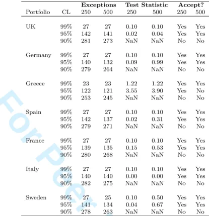
Exceptions Test Statistic Accept?
Portfolio CL 250 500 250 500 250 500
UK 99% 27 27 0.10 0.10 Yes Yes
95% 142 141 0.02 0.04 Yes Yes
90% 281 273 NaN NaN No No
Germany 99% 27 27 0.10 0.10 Yes Yes 95% 140 132 0.09 0.99 Yes Yes
90% 279 264 NaN NaN No No
Greece 99% 23 23 1.22 1.22 Yes Yes 95% 122 121 3.55 3.90 Yes No
90% 253 245 NaN NaN No No
Spain 99% 27 27 0.10 0.10 Yes Yes 95% 142 137 0.02 0.31 Yes Yes
90% 279 271 NaN NaN No No
France 99% 27 27 0.10 0.10 Yes Yes 95% 139 135 0.15 0.53 Yes Yes
90% 280 268 NaN NaN No No
Italy 99% 27 27 0.10 0.10 Yes Yes 95% 140 140 0.00 0.00 Yes Yes
90% 282 275 NaN NaN No No
Sweden 99% 27 25 0.10 0.50 Yes Yes 95% 141 134 0.04 0.67 Yes Yes
90% 278 263 NaN NaN No No
Table 9: Testing the reliability of the VaR model based on Kupiec’s POF coverage test. Re-turns generated using elliptical copulas. Time horizon = 1 day; 250- and 500-day observation periods.
7
Summary and Conclusion
Because VaR models attempt to capture the behaviour of asset returns in the left tail, it is important that the model is constructed such that it does not underestimate the proportion of outliers and hence the true VaR. The normality assumption of asset returns might severely underestimate the true VaR because extreme values are assumed to be very unlikely to occur. Therefore for a reliable VaR model, it is important to take into account the choice of time horizon, the observation period, and the type of volatility models being used. We construct our VaR model using copulas with a DCC M-GARCH volatility model for a time horizon of one day. We then check the reliability of the model by back-testing on a window of 250 and 500 observation periods and record the number of exceptions produced.
As the observation period increases from 250 to 500 days at a 99% confidence level, the number of exceptions produced is unchanged using elliptical copulas with the exception of
3 4 5 6 7 8 9 10 11 12 13 14 15 16 17 18 19 20 21 22 23 24 25 26 27 28 29 30 31 32 33 34 35 36 37 38 39 40 41 42 43 44 45 46 47 48 49 50 51 52 53 54 55 56 57 58
For Peer Review Only
Sweden, which exhibits a difference of 2. With Archimedean copulas, there is a difference of 1, 1, and 2 for the UK, Germany and Sweden, respectively, at the 99% confidence level. The number of exceptions produced is also very close to the expectation (i.e., 29) with the exception of Greece for the elliptical Student’s-t copula. This suggests that the model at a 99% confidence level captures VaR extremely well because the difference in exceptions is very minimal or zero.
At the 95% confidence level, there is a significant difference between the number of exceptions produced in some of the countries when using 250- and 500-observation periods for both Archimedean and elliptical copulas. Although the number of exceptions is quite close to the expectation, 143, the significant difference indicates that there is greater room for error in estimating VaR at the 95% compared with the 99% confidence level. However, back-testing results indicate that the VaR model performed quite well at the 95% confidence level except for the models of Greece in the 500-observation period.
At a 90% confidence level, the difference in the number of exceptions is quite high for both copula families. The tail dependence structure of the portfolio returns is not quite accounted for and hence, the model fails to capture extreme events.
Back-testing results from Kupiec’s POF test confirm the above analysis. The model is accepted at the 99% and 95% confidence levels for both copula families except for in Greece, where the elliptical Student’s-t copula rejects the model at a 95% confidence level with a 500-day observation period. At a 90% confidence level, Kupiec’s POF test rejects the model for both copula families.
For the standard normal hypothesis test and Basel “traffic light” test, we perform one-and two-tailed tests. Although Basel is only concerned with the underestimation of risk, we performed a two-tailed test to make sure that the model does not overestimate risk and thereby result in excess capital being provided (Best, 2000). The model is accepted in all cases for both one-tailed and two-tailed tests. However, for both Archimedean and elliptical copulas, the Basel “traffic light” test places the VaR model in the yellow zone for a
two-2 3 4 5 6 7 8 9 10 11 12 13 14 15 16 17 18 19 20 21 22 23 24 25 26 27 28 29 30 31 32 33 34 35 36 37 38 39 40 41 42 43 44 45 46 47 48 49 50 51 52 53 54 55 56 57 58 59
For Peer Review Only
tailed test when using 250- and 500-observation periods, suggesting that there might be some instances of overestimation of risk since for a one-tailed test the model falls in the green zone in all instances.
It is also important to note that the standard normal hypothesis test and the Basel “traffic light” test do not specify whether the number of exceptions produced is too small. That is, the model will not be rejected if the number of exceptions is too low, which would lead to overestimation of VaR. Kupiec’s POF test rejects the model if the number of exceptions produced is too high or too low. This is why the standard normal hypothesis test and Basel “traffic light” test fail to reject the model at the 90% confidence level. Thus, from the banks perspective, Kupiec’s POF test is preferable and superior because it accounts for both underestimation and overestimation of risk. Back-testing results also suggest that the type of copula family used (i.e., elliptical or Archimedean) to model the dependence structure does not have a strong effect when dealing with quantile VaRs. The results are quite similar based on the number of exceptions produced.
This study suggests a challenging yet possible development in the world of risk manage-ment, that is, to design a model based on the Basel requirements that detects when the number of exceptions produced by a VaR model is too low.
References
Alexander, C., 2008. Market Risk Analysis, Practical Financial Econometrics. Vol. II. John Wiley & Sons.
Bauwens, L., Laurent, S., Rombouts, J. V., 2006. Multivariate garch models: a survey. Journal of applied econometrics 21 (1), 79–109.
Berkowitz, J., Christoffersen, P., Pelletier, D., 2011. Evaluating value-at-risk models with desk-level data. Management Science 57 (12), 2213–2227.
3 4 5 6 7 8 9 10 11 12 13 14 15 16 17 18 19 20 21 22 23 24 25 26 27 28 29 30 31 32 33 34 35 36 37 38 39 40 41 42 43 44 45 46 47 48 49 50 51 52 53 54 55 56 57 58
For Peer Review Only
Berkowitz, J., Obrien, J., 2002. How accurate are value-at-risk models at commercial banks? The journal of finance 57 (3), 1093–1111.
Best, P., 2000. Implementing value at risk. John Wiley & Sons.
Bob, N. K., 2013. Value at risk estimation. a garch-evt-copula approach. Mathematiska institutionen.
Bollerslev, T., Engle, R. F., Nelson, D. B., 1994. Arch models. Handbook of econometrics 4, 2959–3038.
Cherubini, U., Luciano, E., 2001. Value-at-risk trade-off and capital allocation with copulas. Economic notes 30 (2), 235–256.
Cherubini, U., Luciano, E., Vecchiato, W., 2004. Copula methods in finance. John Wiley & Sons.
Cherubini, U., Mulinacci, S., Gobbi, F., Romagnoli, S., 2011. Dynamic Copula methods in finance. Vol. 625. John Wiley & Sons.
Clayton, D. G., 1978. A model for association in bivariate life tables and its application in epidemiological studies of familial tendency in chronic disease incidence. Biometrika 65 (1), 141–151.
Drehmann, M., 2007. Conference–2007 discussion in conference 2007.
Embrechts, P., Lindskog, F., 2003. A. mcneil (2001b),modelling dependence with copulas and applications to risk management,. Preprint, ETH Zurich.
Embrechts, P., McNeil, A., 1999. D. straumann [1999], correlation and dependency in risk management: properties and pitfalls, departement of mathematik, ethz. Tech. rep., Z¨urich, Working Paper. 2 3 4 5 6 7 8 9 10 11 12 13 14 15 16 17 18 19 20 21 22 23 24 25 26 27 28 29 30 31 32 33 34 35 36 37 38 39 40 41 42 43 44 45 46 47 48 49 50 51 52 53 54 55 56 57 58 59
For Peer Review Only
Embrechts, P., McNeil, A., Straumann, D., 2002. Correlation and dependence in risk man-agement: properties and pitfalls. Risk manman-agement: value at risk and beyond, 176–223. Engle, R., 2002. Dynamic conditional correlation: A simple class of multivariate
general-ized autoregressive conditional heteroskedasticity models. Journal of Business & Economic Statistics 20 (3), 339–350.
Engle, R. F., Kroner, K. F., 1995. Multivariate simultaneous generalized arch. Econometric theory 11 (01), 122–150.
Fantazzini, D., 2008. Dynamic copula modelling for value at risk. Frontiers in Finance and Economics 5 (2), 72–108.
Fengler, M. R., Herwartz, H., 2008. Multivariate volatility models. Springer.
Frank, M. J., 1979. On the simultaneous associativity off (x, y) andx+y- f (x, y). Aequationes mathematicae 19 (1), 194–226.
Frey, R., McNeil, A. J., McNeil, A. J., McNeil, A. J., 2001. Modelling dependent defaults. ETH, Eidgen¨ossische Technische Hochschule Z¨urich, Department of Mathematics.
Ghalanos, A., 2015. The rmgarch models: Background and properties.(version 1.2-8). URL http://cran. r-project. org/web/packages/rmgarch/index. html.
Gumbel, E. J., 1960. Bivariate exponential distributions. Journal of the American Statistical Association 55 (292), 698–707.
Holton, G. A., 2002. History of value-at-risk.
Holton, G. A., 2014. Value-at-risk: theory and practice. e-book at http://value-at-risk.net. Huang, J.-J., Lee, K.-J., Liang, H., Lin, W.-F., 2009. Estimating value at risk of portfolio by
conditional copula-garch method. Insurance: Mathematics and economics 45 (3), 315–324.
3 4 5 6 7 8 9 10 11 12 13 14 15 16 17 18 19 20 21 22 23 24 25 26 27 28 29 30 31 32 33 34 35 36 37 38 39 40 41 42 43 44 45 46 47 48 49 50 51 52 53 54 55 56 57 58
For Peer Review Only
Jorion, P., 2007. Value at risk: the new benchmark for managing financial risk. Vol. 3. McGraw-Hill New York.
Kuester, K., Mittnik, S., Paolella, M. S., 2006. Value-at-risk prediction: A comparison of alternative strategies. Journal of Financial Econometrics 4 (1), 53–89.
Li, D. X., 1999. On default correlation: A copula function approach. Available at SSRN 187289.
Malz, A. M., 2011. Financial risk management: Models, history, and institutions. Vol. 538. John Wiley & Sons.
McNeil, A. J., Frey, R., 2000. Estimation of tail-related risk measures for heteroscedastic financial time series: an extreme value approach. Journal of empirical finance 7 (3), 271– 300.
Nelsen, R. B., 2007. An introduction to copulas. Springer Science & Business Media.
on Banking Supervision, B. C., 1996. Supervisory framework for the use of” backtesting” in conjunction with the internal models approach to market risk capital requirements. Bank for International Settlements.
Patton, A. J., 2004. On the out-of-sample importance of skewness and asymmetric depen-dence for asset allocation. Journal of Financial Econometrics 2 (1), 130–168.
Resti, A., 2008. Pillar II in the New Basel Accord: the challenge of economic capital. Risk books.
Sheikh, A. Z., Qiao, H., 2010. Non-normality of market returns: A framework for asset allocation decision making (digest summary). Journal of Alternative Investments 12 (3), 8–35. 2 3 4 5 6 7 8 9 10 11 12 13 14 15 16 17 18 19 20 21 22 23 24 25 26 27 28 29 30 31 32 33 34 35 36 37 38 39 40 41 42 43 44 45 46 47 48 49 50 51 52 53 54 55 56 57 58 59
For Peer Review Only
Silva Filho, O. C., Ziegelmann, F. A., Dueker, M. J., 2014. Assessing dependence between financial market indexes using conditional time-varying copulas: applications to value at risk (var). Quantitative Finance 14 (12), 2155–2170.
Silvennoinen, A., Ter¨asvirta, T., 2009. Multivariate garch models. In: Handbook of financial time series. Springer, pp. 201–229.
Sklar, M., 1959. Fonctions de r´epartition `a n dimensions et leurs marges. Universit´e Paris 8. So, M. K., Philip, L., 2006. Empirical analysis of garch models in value at risk estimation.
Journal of International Financial Markets, Institutions and Money 16 (2), 180–197. Tsay, R. S., 2005. Analysis of financial time series. Vol. 543. John Wiley & Sons.
Tsay, R. S., 2013. Multivariate Time Series Analysis: With R and Financial Applications. John Wiley & Sons.
Tse, Y. K., Tsui, A. K. C., 2002. A multivariate generalized autoregressive conditional heteroscedasticity model with time-varying correlations. Journal of Business & Economic Statistics 20 (3), 351–362.
Yan, J., et al., 2007. Enjoy the joy of copulas: with a package copula. Journal of Statistical Software 21 (4), 1–21. 3 4 5 6 7 8 9 10 11 12 13 14 15 16 17 18 19 20 21 22 23 24 25 26 27 28 29 30 31 32 33 34 35 36 37 38 39 40 41 42 43 44 45 46 47 48 49 50 51 52 53 54 55 56 57 58
For Peer Review Only
Time plots of daily log return series for French stocks indicating presence of volatility clustering. 291x164mm (72 x 72 DPI) 2 3 4 5 6 7 8 9 10 11 12 13 14 15 16 17 18 19 20 21 22 23 24 25 26 27 28 29 30 31 32 33 34 35 36 37 38 39 40 41 42 43 44 45 46 47 48 49 50 51 52 53 54 55 56 57 58 59
For Peer Review Only
Time plots of daily log return series for German stocks indicating presence of volatility clustering.
291x164mm (72 x 72 DPI) 3 4 5 6 7 8 9 10 11 12 13 14 15 16 17 18 19 20 21 22 23 24 25 26 27 28 29 30 31 32 33 34 35 36 37 38 39 40 41 42 43 44 45 46 47 48 49 50 51 52 53 54 55 56 57 58
For Peer Review Only
Time plots of daily log return series for Greek stocks indicating presence of volatility clustering.
291x164mm (72 x 72 DPI) 2 3 4 5 6 7 8 9 10 11 12 13 14 15 16 17 18 19 20 21 22 23 24 25 26 27 28 29 30 31 32 33 34 35 36 37 38 39 40 41 42 43 44 45 46 47 48 49 50 51 52 53 54 55 56 57 58 59
For Peer Review Only
Time plots of daily log return series for Italian stocks indicating presence of volatility clustering. 291x164mm (72 x 72 DPI) 3 4 5 6 7 8 9 10 11 12 13 14 15 16 17 18 19 20 21 22 23 24 25 26 27 28 29 30 31 32 33 34 35 36 37 38 39 40 41 42 43 44 45 46 47 48 49 50 51 52 53 54 55 56 57 58
For Peer Review Only
Time plots of daily log return series for Spanish stocks indicating presence of volatility clustering. 291x164mm (72 x 72 DPI) 2 3 4 5 6 7 8 9 10 11 12 13 14 15 16 17 18 19 20 21 22 23 24 25 26 27 28 29 30 31 32 33 34 35 36 37 38 39 40 41 42 43 44 45 46 47 48 49 50 51 52 53 54 55 56 57 58 59
For Peer Review Only
Time plots of daily log return series for Swedish stocks indicating presence of volatility clustering. 291x164mm (72 x 72 DPI) 3 4 5 6 7 8 9 10 11 12 13 14 15 16 17 18 19 20 21 22 23 24 25 26 27 28 29 30 31 32 33 34 35 36 37 38 39 40 41 42 43 44 45 46 47 48 49 50 51 52 53 54 55 56 57 58
For Peer Review Only
Time plots of daily log return series for UK stocks indicating presence of volatility clustering. 291x164mm (72 x 72 DPI) 2 3 4 5 6 7 8 9 10 11 12 13 14 15 16 17 18 19 20 21 22 23 24 25 26 27 28 29 30 31 32 33 34 35 36 37 38 39 40 41 42 43 44 45 46 47 48 49 50 51 52 53 54 55 56 57 58 59