Borrowing Constraints, Entrepreneurial
Risks, and the Wealth Distribution in a
Heterogeneous Agent Model
Christiane Clemens
Maik Heinemann
FEMM Working Paper No. 8, February 2008
O
TTO
-
VON
-G
UERICKE
-U
NIVERSITY
M
AGDEBURG
F
ACULTY OF
E
CONOMICS AND
M
ANAGEMENT
F E M M
Faculty of Economics and Management Magdeburg
Working Pa per Se ries
Otto-von-Guericke-University Magdeburg Faculty of Economics and Management P.O. Box 4120 39016 Magdeburg, Germany
Borrowing Constraints, Entrepreneurial Risks,
and the Wealth Distribution in a
Heterogeneous Agent Model
Christiane Clemens∗ University of Magdeburg Maik Heinemann∗∗ University of Lüneburg February 27, 2008 Abstract
This paper deals with credit market imperfections and idiosyncratic risks in a two–sector heterogeneous agent dynamic general equilibrium model of oc-cupational choice. We focus especially on the effects of tightening financial constraints on macroeconomic performance, entrepreneurial risk–taking, and social mobility. Contrary to many models in the literature, our comparative static results cover the entire range of borrowing constraints, from complete markets to a perfectly constrained economy. In our baseline model, we find substantial gains in output, welfare, and wealth equality associated with re-laxing the constraints, but argue that it might also prove worthwhile to ex-amine the marginal gains from credit market improvements. Interestingly, the amount of entrepreneurial activity and social mobility increases if borrowing constraints become more tight. These results can be attributed to the general equilibrium nature of our approach, where optimal firm sizes and the demand for credit are determined endogenously. The comparative static results on the entrepreneurship rate and social mobility respond sensitively to a change in income persistence.
Keywords: DSGE model, wealth distribution, occupational choice, borrowing constraints JEL classification: C68, D3 , D8, D9, G0, J24
∗Otto–von–Guericke University Magdeburg, Germany,Christiane.Clemens@ww.uni-magdeburg.de ∗∗University of Lüneburg, Germany,heinemann@uni-lueneburg.de
1
IntroductionThis paper examines the effects of credit market imperfections and idiosyncratic risks on occupational choice, macroeconomic performance, as well as on the income and wealth distribution. Our analysis contributes to recent literature on dynamic stochastic heterogeneous agent general equilibrium models concerned with risk and distributional dynamics, for instance,Quadrini(2000),Meh(2005),Bohá˘cek(2006,
2007) andCagetti and De Nardi(2006a,b,c).
We develop a model which combines the features of aHuggett(1993) /Aiyagari
(1994)–type economy with occupational choice under risk à laKihlstrom and Laffont
(1979) andKanbur(1979a,b), and the two–sector approach of Romer(1990), but without endogenous growth. In each period of time, the risk–averse agents choose between between two alternative occupations. They either set up an enterprise in the intermediate goods industry which is characterized by monopolistic competi-tion.1 Or, they supply their labor endowment to the production of a final good in a perfectly competitive market. Producers of the final good use capital and labor inputs, and differentiated varieties of the intermediate good. All households are subject to an income risk. Managerial ability and productivity as a worker follow independent random processes. Entrepreneurial activity is rewarded with a higher expected income. Similar toLucas(1978), there is no aggregate risk.
The economic performance in the intermediate goods industry crucially depends on two factors: uncertainty and credit constraints. Business owners face an firm– specific productivity shock, and there are no markets available for pooling the idio-syncratic risks. Physical capital is the single input factor in the intermediate goods industry. Entrepreneurs maximize their profits if their business operates at the opti-mal firm size. For an individual wealth too sopti-mall to maintain the optiopti-mal firm size, the firm–owner would want to borrow the remaining amount on the credit market, where he might be subject to financial constraints. If the entrepreneur is wealthy enough, he operates his business at the profit–maximizing level and supplies the rest of his wealth to the capital market. Contrary to many models in the literature the two–sector general equilibrium approach allows us to endogenously determine optimal firm sizes and credit constraints, and we do not have to fall back on fixed investment projects (or entry costs respectively) in order to analyze the effects of credit market frictions. There is no further portfolio choice in our framework. To this end, our approach draws a simple picture of the empirical result, stated by
Heaton and Lucas(2000), that the entrepreneurial households’ business wealth on average constitutes a relevant fraction of their total wealth.
Capital accumulation plays a twofold role in the context outlined above: On the one hand, it endows individuals with the wealth necessary to set–up and
erate a firm. On the other hand, buffer–stock saving provides a self–insurance on intertemporal markets against the non–diversifiable income risk. Accordingly, we find that wealthier households are more likely to be members of the entrepreneurial class than poorer ones and there is a marked concentration of wealth in the hands of entrepreneurs which is consistent with recent empirical findings (cf. Quadrini,
1999; Holtz-Eakinet al.,1994a). Upward mobility of entrepreneurs in our model is primarily accumulation driven. The riskiness of entrepreneurial incomes looses its importance for occupational choice once the household’s income share generated from profits declines relative to his capital income. Nevertheless, in accordance with
Hamilton(2000), many entrepreneurs of our model enter and persist in business de-spite the fact that they have lower initial earnings than average wage incomes.
We are especially interested in the question of how tightening financial con-straints affects the macroeconomic general equilibrium regarding aggregate output, the sectoral allocation of capital and labor, factor prices, the income and wealth dis-tribution, occupational choice as well as the between–group mobility of households. Our comparative static analysis covers the entire range of borrowing constraints, from complete markets to a perfectly constrained economy. This is a novel approach since many models of the literature consider a fixed equity–to–loan ratio, or rest with a comparison of complete vs. a specific incomplete market, or they focus on the no–credit market scenario. We find that increasing the degree of constraint is ac-companied by substantial losses in aggregate output, consumption, wealth holdings, and welfare, while wealth inequality increases.
Reviewing the empirical evidence, there is a strong support for the hypothe-sis that borrowing constraints are an impediment to entering entrepreneurship; see Evans and Leighton (1989), Evans and Jovanovic (1989), Holtz-Eakinet al.
(1994b), Blanchflower and Oswald (1998), Moskowitz and Vissing-Jørgensen
(2002), as well asDesaiet al.(2003).
Gentry and Hubbard(2004) point out that external financing has important im-plications for individual investment and saving. This evidence is challenged by
Hurst and Lusardi (2004), who find that the likelihood of entering entrepreneur-ship relative to initial wealth is flat over a large range of the wealth distribution and increasing only for higher wealth levels of workers.
The general equilibrium nature of our approach generates surprising and almost counter–intuitive results regarding the impact of credit constraints on occupational choice under risk. If the idiosyncratic risks are serially correlated, more house-holds choose the entrepreneurial profession in the constrained compared to the unconstrained economy which is accompanied by a reduction in the average firm size, both results contradicting findings reported inCagetti and De Nardi(2006a). Wealth inequality does not necessarily decline if we relax borrowing constraints. Ad-ditionally, we observe an increase in between–group mobility, if credit constraints become more binding. Workers and entrepreneurs with high individual productivity
tend to remain in their present occupation, whereas low productivity individuals are more likely to switch between professions.
These results reverse completely, if we consideriidshocks to individual produc-tivity. In this case, credit constraints actually are an impediment to entrepreneurship. Only the wealthy workers tend to switch between occupations and between–group mobility drops down sharply for an increase in the tightness of credit constraints. Re-garding the functional distribution of income, we find that credit constraints have a redistributive effect by raising the profit income share at the cost of capital incomes. The results indicate that the stochastic nature of the underlying idiosyncratic shocks also plays an important role for the explanation of the general equilibrium effects of financial constraints and credit market imperfections.
Recent contributions in this area of research suffer from several shortcomings which our approach aims to overcome. In Quadrini (2000), occupational choice and the level of entrepreneurship is (more or less) entirely governed by the un-derlying productivity shocks. Li (2002) and Bohá˘cek (2006) discuss economies with a single sector of production which does not allow for factor movements be-tween industries and therefore neglects factor substitution. In our model, produc-ers of the intermediate and the final good are subject to competition, especially with respect to capital demand. Our approach does not have fixed entry costs (in terms of discrete investment projects) of entrepreneurship as in Ghataket al.
(2001),Fernández-Villaverdeet al.(2003) orClementi and Hopenhayn(2006) . In-stead, we have an endogenously determined optimal firm size and no discontinuities in individual credit demand. Occupational choice, entrepreneurial activity and per-formance crucially depend on monopoly profits, market shares and relative factor scarcity in the two sectors of production. Also different to Cagetti and De Nardi
(2006a) or Kitao (2008), the entrepreneurs of our economy are essential for ag-gregate output. We will show that the interdependence of sectors is important for the general equilibrium results on occupational choice, between–group mobility and the income and wealth distribution, and contributes to the explanation of the sometimes counter–intuitive effects of borrowing constraints outlined above. To this end, the present paper is an extended version ofClemens and Heinemann(2006) andClemens(2008), where we focus on the relation between entrepreneurial risk– taking and growth but do not consider financial constraints.
The paper is organized as follows: Section2develops the two–sector model. We describe the equilibrium associated with a stationary earnings and wealth distribu-tion. Because the formal structure of the model does not allow for analytical solu-tions, we perform numerical simulations of a calibrated model in order to examine the general equilibrium effects of an increase in the tightness of credit constraints. Section3gives information on the calibration procedure and related empirical ev-idence. Section4 discusses the simulation results. Section5 concludes. Technical details are relegated to the Appendix.
2
The Model 2.1 OverviewWe consider a neoclassical growth model with two sectors of production. Drawing fromQuadrini(2000) andRomer(1990), we consider a corporate sector with per-fectly competitive large firms who hire capital and labor services and use an inter-mediate good in order to produce a homogeneous output which can be consumed or invested respectively. The intermediate goods industry (noncorporate sector) con-sists of a large number of small firms operating under the regime of monopolistic competition. Each firm in this sector is owned and managed by an entrepreneur. Both sectors of production are essential.
Market activity in the intermediate goods industry is constrained. In order to run the business at the profit–maximizing firm size, entrepreneurs either possess sufficient wealth of their own, or they need to compensate for their lack of eq-uity by borrowing on the credit market, where they might be subject to borrowing constraints. The two–sector setting allows us to endogenously relate financial con-straints to individual characteristics and overall market activity.
The economy is populated by a continuum [0,1]of infinitely–lived households, each endowed with one unit of labor. In each period of time, individuals follow their occupation predetermined from the previous period and make a decision regarding their future profession, which is either to become producers of the intermediate good or to supply their labor services to the production of the final good. Labor efficiency as well as entrepreneurial productivity are idiosyncratic random variables. Regarding the associated income risk, we assume that wage incomes are less risky than profit incomes. There is no aggregate risk.
With respect to the timing of events, we assume that individual occupational choice takes place before the resolution of uncertainty. Once the draw of nature has occurred, entrepreneurs as well as workers in the final goods sector know their individual productivity. Those monopolists, who now discover their own wealth being too low to operate at the optimal firms size, will express their capital demand on the credit market, probably become subject to credit–constraints, and then start production. After labor and profit income is realized, the households decide on how much to consume and to invest. There is no capital income risk and no risk of production in the corporate sector.
2.2 Final Goods Sector
The representative firm of the final goods sector produces a homogeneous goodY using capital KF, labor L, and varieties of an intermediate good x(j),j∈[0,λ] as inputs. Production in this sector takes place under perfect competition and the price
ofY is normalized to unity. The production function is of the generalized CES–form2
Y =KFγL1−γ1−α Z λ
0 x(j)
αdj, 0<α<1, 0<γ<1. (1) Each type of intermediate good employed in the production of the final good is identified with one monopolistic producer in the intermediate goods sector. Con-sequently, the number of different types is identical with the population share λ of entrepreneurs in the population. The number of entrepreneurs is determined endogenously through occupational choices of the agents, which will be described below. Additive–separability of (1) in intermediate goods ensures that the marginal product of input jis independent of the quantity employed of j= j. Intermediate goods are close but not perfect substitutes in production.
The profit of the representative firm in the final goods sector,πF, is given in each period by
πF =Y−wL−(r+δ)KF− Z λ
0 p(j)x(j)dj, (2)
where p(j) denotes the price of intermediate good j. We further assume physical capital to depreciate over time at the constant rate δ, such that the interest factor is given byR=1+r−δ. Optimization yields the profit maximizing factor demands consistent with marginal productivity theory
KF = (1−α)γr+Yδ , (3) L= (1−α)(1−γ)Yw (4) x(j) =KFγL1−γ α p(j) 1/(1−α) . (5)
The monopolistic producer of intermediate good x(j) faces the isoelastic demand function (5), where the direct price elasticity of demand is given by −1/(1−α). Condition (4) describes aggregate labor demand in efficiency units. Equation (3) is the final good sector demand for capital services.
2.3 Intermediate Goods Sector
The intermediate goods sector consists of the population fractionλof entrepreneurs who self–employ their labor endowment by operating a monopolistic firm. Each monopolist produces a single variety j of the differentiated intermediate good by
2All macroeconomic variables are time–dependent. For notational convenience, we will drop the
employing capital from own wealth and borrowed resources according to the iden-tical constant returns to scale technology of the form
x(j) =θ(i)ek(i). (6) Firm owners are heterogeneous in terms of their talent as entrepreneurs. They differ with respect to the realization of an idiosyncratic productivity shock θ(i)e which is assumed to be non–diversifiable and uncorrelated across firms. We will give more details on the properties of the shock below. Entrepreneurs hire capital after the draw of nature has occurred. The firm problem essentially is a static one. Under perfect competition of the capital market, the producer treats the rental rate to capital as exogenously given and maximizes his profit
π(k(i),θ(i)e) =p(j)x(j)−(r+δ)k(i). (7) Utilizing the demand function for intermediate good type–i, (5), and the pro-duction technology (6), the optimal firm decision can be expressed in terms of the optimal firm sizek(i)∗as a function of capital input, which is given by:
k(i)∗=L(θ(i) e)1−αα γw (1−γ)(r+δ) γ . (8)
Because capital demand takes place after the draw of nature has occurred, there is no individual capital risk and no under–employment of input factors. The optimal firm size increases with random individual productivityθ(i)e, such that more pro-ductive business owners demand more capital on the capital market. Labor input in efficiency units determines the optimal firm size by means of the demand function for intermediate good type j. Aggregate employment is a weighted average and depends on the size of the labor force 1−λ, i.e. the population fraction of agents choosing the occupation of a worker, and the idiosyncratic shock on labor productiv-ityθw. The larger the labor force1−λ, the higher—ceteris paribus—will be aggregate employmentL. This goes along with fewer monopolists in the intermediate goods industry, less competition, and a larger market share, as measured by the optimal firm size.
2.4 Incomes and Equilibrium Income Shares in the Unconstrained Economy Households derive income from three sources: labor income, capital income and monopolistic profits. The technology parameters α and γ determine the division of aggregate income among the three income sources in the absence of financial constraints on entrepreneurial activity. According to marginal productivity theory, we obtain from (1) a labor share of (1−α)(1−γ) and a capital share of(1−α)γ. The remaining income shareαaccrues to the two types of income generated in the intermediate goods sector, and splits on profits withα(1−α)and capital income with α2, respectively, such that the economy–wide capital share amounts to(1−α)γ+α2.
2.5 Capital Market and Financial Constraints
Firms of the final goods sector and the intermediate goods industry differ with re-spect to access to financial markets. While the first are not constrained in their financing, the latter face greater difficulties in diversifying the risk from their en-trepreneurial activities and, moreover, are subject to borrowing constraints. En-trepreneurs of the intermediate goods industry, who are wealth–constrained in op-erating their business at the optimal size (8), seek external financing from finan-cial intermediaries. The credit market is imperfect with respect to lenders not be-ing able to enforce loan–repayment due to limited commitment of borrowers (cf.
Banerjee and Newman,1993). In order not to default on loan contracts, borrowing amounts are limited, and individual wealth acts as collateral. We do not explic-itly model financial intermediaries and assume that there is no difference between borrowing and lending rates.
In case of default, the financial intermediator is able to seize a fraction of the borrowers gross capital income (1+r)a(i). Alternatively, one could assume the entrepreneur’s profit income to act as collateral. The major difference between the two approaches is that, in the first case, borrowing amounts are entirely determined by the debtors individual wealtha(i), whereas in the second, they also depend on his entrepreneurial talentθ(i)e, which might be private information. We will discuss the consequences of the second formulation in a separate treatment below.
The creditor will lend to the borrower only the amount consistent with the bor-rower’s incentive compatibility constraint, such that it is in the borbor-rower’s interest to repay the loan and there is no credit default in equilibrium.
Letk(i) =a(i) +b(i) be the firm size an entrepreneur is able to operate at from own wealtha(i)and borrowed resourcesb(i). This operating capitalk(i)is not nec-essarily equal to the optimal firm sizek(i)∗determined in (8). An entrepreneur with individual wealtha(i)lower thank(i)∗would want to borrow the amountk(i)∗−a(i). In case ofk(i)<k(i)∗ the firm faces a borrowing constraint. Incentive compatibility requires that it is never optimal for the borrower to default, that is
π(i) + (1+r)a(i)π(i) +b(i)(1+r) + (1−φ)(1+r)a(i)
b(i)≤φa(i). (9)
The borrowing amount is limited such that the maximum possible loan is propor-tional to the borrowers individual wealtha(i). The parameterφis a measure for the extent to which a lender can use the borrower’s wealth income as collateral. Credit constraints become less tight with rising φ and vanish for large φ. The limiting cases consequently reflect the two cases of either complete enforceability(φ→∞) or no enforceability (φ=0), such that in the first case the borrower is considered solvent, whereas in the second one he is not. The sensitivity of results with respect to changesφconstitutes the major part of our numerical analysis later on.
Summing up, the operating firm sizek(i)of entrepreneuriwith productivityθ(i)e and wealtha(i)can be written as:
k(i) =k(θ(i)e,a(i)) =min[a(i),k(i)∗] +min[φa(i),k(i)∗−min[a(i),k(i)∗]]. (10) The first term on the RHS of (10) reflects the size of a firm not seeking external financing, where the business owner simply rests with his own wealth. The second term describes the amount an entrepreneur with wealth a(i) will actually borrow. The subsequent numerical analysis shows that the high–productivity entrepreneurs are more likely to be constrained than the low–productivity ones, because the opti-mal firm size and henceforth the capital demand increase in the productivity shock. An entrepreneur, whose individual wealth exceeds the level needed to operate his business at the optimal firm size will lend the amount a(i)−k(i)∗ on the cap-ital market at the equilibrium interest rate. The supply side of the capcap-ital market altogether consists of those entrepreneurs whose wealth exceeds their individual optimal firm size and of workers, who supply their savings. On the demand side we have the credit–constrained entrepreneurs and firms from the final goods indus-try. From this follows immediately that the size of the intermediate goods industry relative to the final goods sector essentially depends on occupational choice and individual wealth accumulation, both determined endogenously in equilibrium. 2.6 Idiosyncratic Risks
In each period of time, workers are endowed with one unit of raw labor and are subject to an idiosyncratic shockθw affecting labor supply in efficiency units, and exposing each of them to an uninsurable income risk. For simplicity, we assume that labor productivity θw evolves according to a first–order Markov process with
h=1,...,mstates, and θw,h>0. The transition matrix associated with the Markov process isPw.
Entrepreneurial productivity θe also evolves according to a first–order Markov process withh=1,...,mdifferent states θe,1,...,θe,m; θe,h>0, and transition
prob-ability Pe. Since agents can either be workers or entrepreneurs, it is possible to identify the occupational status of an agent with his productivity in the respective occupation. We assume worker productivities to be more evenly distributed than managerial skills, such that profit incomes in general are more risky than wage incomes. As is well–known from the literature, entrepreneurs on average are com-pensated with a positive income differential (aka ‘risk premium’) for bearing the production risk.
By modeling two distinct random processes for workers and entrepreneurs, we take into account that the two professions demand different talents, for instance spe-cific managerial skills. We assume the processesθw andθe to be uncorrelated, such that for an individual the conditional expectation of entrepreneurial productivity is
independent of the labor efficiency, if employed as a worker.3 A high productivity as a worker in the present does not necessarily indicate an equivalently high future productivity as an entrepreneur, if the individual should decide to switch between occupations in the next period. The associated probabilities are summarized in a
m×mtransition matrices Pn,n describing the transition from productivity stateθn,h
to stateθn,h forh,h=1,...,m,n=e,wandn=n.
We consider two different specifications regarding the Markov processes for en-trepreneurial talent and worker efficiency respectively. Shocks of the first setting are serially correlated, thus introducing a certain persistence in individual income processes. Currently highly productive workers and entrepreneurs are more likely to be highly productive in the future. The individual is able to infer from his present productivity how his future productivity in the same occupation will be. Shocks of the second setting are iid. Although empirically not supported, when confronted with the data (cf.Guvenen,2007, and references therein), the second setting allows us to illustrate the role intertemporal income persistence has for occupational choice and social mobility.
2.7 Intertemporal Decision and Occupational Choice
Each householdihas preferences over consumption and maximizes discounted ex-pected lifetime utility
E0 ∞
∑
t=0 βtU[c t(i)] 0<β<1.E0 is the expectation operator conditional on information at date 0 and β is the
discount factor. Individuals are assumed to be identical with respect to their pref-erences regarding momentary consumption c(i) which are described by constant relative risk aversion
U[c(i)] = ⎧ ⎪ ⎨ ⎪ ⎩ c(i)1−ρ 1−ρ forρ>0,ρ=1 lnc(i) forρ=1,
whereρdenotes the Arrow/Pratt measure of relative risk aversion.
In each period, the single household is endowed with a unit of raw labor and— in addition to his intertemporal decision—makes a choice on his future occupation, which is either to become a self–employed producer of an intermediate good in the monopolistically competitive market or to supply his labor services in efficiency units inelastically to the production of the final good. Occupational choice, once made in a certain period, is irreversible.
LetVw(a(i),θ(i)w,h)denote the optimal value function of an agent currently being a worker with wealtha(i), who is in productivity stateθw,h,h=1,...,m. If he decides
to remain a worker, his productivity evolves according to the transition matrix Pw of the underlying Markov process with states θw,1,...,θw,m. If, instead, he decides
to become an entrepreneur in the following period, his next period productivityθe is determined by the transition matrixPw,e. For analytical convenience, individual asset holdings are bounded from below, the lowest possible wealth level set toa=0. The associated maximized value function for a typical individual currently being a worker is given by Vw(a(i),θ(i)w,h) = max c(i)0,a(i)a U[c(i)] +β max ξ∈{0,1} EVwa(i),θ(i)w,h|θ(i)w,h,EVea(i),θ(i)e,h s.t. a(i)= (1+r)a(i) +θ(i)w,hw−c(i). (11) ξis a boolean variable which takes on the values0or1, depending on whether or not the agent decides to switch between occupations. r andw denote the equilibrium returns to capital and labor in efficiency units, which are constant over time for a stationary distribution of wealth and occupational statuses over agents. The optimal decision associated with the problem (11) is described by the two decision rules for individual asset holdings a(i)w=aw(a(i),θ(i)w,h) and the future professional state ξ(i)
w=ξw(a(i),θ(i)w,h).
LetVe(a(i),θ(i)e,h)denote the maximized value function of an entrepreneur with wealth a(i) in productivity state θ(i)e,h, who faces a decision problem similar to those of a worker. If he decides to remain an entrepreneur, his productivity evolves according to the transition matrixPe of the underlying Markov process with states θe,1,...,θe,m. If, instead, he decides to switch between occupations by becoming a
worker in the next period, his future productivity θw is determined by the transi-tion matrix Pe,w. With k(θ(i)e,h)∗ denoting the optimal firm size, the intertemporal problem of an entrepreneur currently in productivity stateθ(i)e,h, can be written as
Ve(a(i),θ(i)e,h) = max c(i)0,a(i)a U[c(i)] +β max ξ∈{0,1} EVea(i),θ(i)e,h|θ(i)e,h,EVwa(i),θ(i)w,h s.t. a(i)= (1+r)a(i) +π(k(i),θ(i)e,h)−c(i)
k(i) =min[a(i),k(θ(i)e,h)∗] +min[φa(i),k(θ(i)e,h)∗−min[a(i),k(θ(i)e,h)∗]] π(θ(i)e,h,k(i)) =p(x(i))x(θ(i)e,h,k(i))−(r+δ)k(i)
(12) Again,ξis a boolean variable, indicating the agent’s decision on leaving or remaining in his present occupation. The optimal decision is described by the decision rules
for individual asset holdingsa(i)e=ae(a(i),θ(i)e,h)and the future professional state ξ(i)
e=ξe(a(i),θ(i)e,h).4
In general, our model generates the same implications for individual savings and wealth accumulation under risk as, for instance, discussed inAiyagari (1994) or Huggett (1996). Similar toQuadrini (2000) we additionally consider occupa-tional choice. Consequently, wealth accumulation plays a two–fold role: On the one hand, the shocks to worker efficiency and entrepreneurial productivity generate an income risk which households respond to with buffer–stock saving. On the other hand, higher wealth levels protect entrepreneurs against the danger of being sub-ject to financial constraints. In terms ofSandmo(1970) there is only an income but no capital risk in our model, such that the share of risky incomes in total household income declines with growing wealth. Accordingly, the importance of risky prof-its providing negative incentives towards entrepreneurship fades for high levels of wealth.
2.8 Stationary Recursive Equilibrium
A stationary recursive competitive general equilibrium is an allocation, where equi-librium prices generate a distribution of wealth and occupations over agents which is consistent with these prices given the exogenous process for the idiosyncratic shocks and the agents’ optimal decision rules.
LetKF,Landx(j)Ddenote the demands of capital, effective labor and interme-diate goods in the final goods sector. We obtain aggregate labor supply by summing up individual labor supplies in efficiency units over the population fraction1−λof workers. Let, furthermore,qh,h=1,...,mdenote probabilities of states θw,h in the equilibrium distribution of labor productivities. The stationary recursive equilibrium is a set of value functionsVw(a,θw),Ve(a,θe), decision rulesaw(a;θw),ξw(a;θw)and
ae(a;θe),ξe(a;θe), pricesw,r,p(j)and a distribution λ,1−λof households over oc-cupations such that:
(i) the decision rulesaw(a;θw),ξw(a;θw)andae(a;θe),ξe(a;θe)solve the workers’ and entrepreneurs’ problems (11) and (12) at pricesw,r,p(j),
(ii) the aggregate demands of consumption, labor, capital and intermediate goods are the aggregation of individual demands. Factor and commodity markets clear at constant prices w,r,p(j), where factor inputs are paid according to
4Note that the value functions (11) and (12) may not be concave because of the boolean variable ξ, indicating binary choice between occupations. Similar toFernández-Villaverdeet al. (2003), we would like to stress that the dynamic programming algorithm underlying our computational modeling does not require concavity but monotonicity to converge to the true value function; see alsoBohá˘cek
their marginal product: Y =C+δK Z 1 0 k(i)di≡K=KF+ Z λ 0 k(i)di Z 1 λ m
∑
h=1 qhθw,h di=L x(j)S=x(j)D,(iii) the stationary distribution Γ(λ,a,Pe,Pw,Pe,w,Pw,e) of agents over individual wealth holdings, occupations and associated productivities is the fixed point of the law of motion which is consistent with the individual decision rules and equilibrium prices. The distributionλ,1−λof agents over occupations is time–invariant.
The decision rules for workers, aw(a,sw), ξw(a,sw), and entrepreneurs, ae(a,se), ξe(a,se), together with the stochastic processes for individual labor productivity and entrepreneurial productivity, determine the stationary distributionΓat equilibrium pricesw,r. The stationary distributionΓgoverns the entrepreneurship rate (i.e. the mass of firms in the intermediate goods sector), the efficiency units of labor sup-plied by workers, capital demand of the intermediate goods sector, and the aggre-gate capital supply, the latter equaling the mean of individual wealth holdings. Once the entrepreneurship rateλis derived, this together with the stationary distribution of entrepreneurial productivities determines the supply of intermediate goods.
3
CalibrationThe model is calibrated to match standard macro data from OECD countries. Table1
summarizes the parameterization of the model. Regarding preferences, we set the discount factorβand the coefficient of relative risk aversionρaccording to estimates from the literature, in order to generate equilibrium interest rates on safe assets consistent with empirical findings (cf.Mehra and Prescott, 1985; Obstfeld,1994). The parameters of production technology,α andγ, are chosen such as to generate an equilibrium labor income share of 0.63 which matches empirical observations e.g. for the U.S. economy (King and Rebelo,1999). The corresponding capital and profit income shares of the frictionless economy(φ→∞) are0.16 and 0.21. PSID data report a income share for entrepreneurs of around 22%. The depreciation rate is fixed at6%, which also is a standard choice in the literature.
The steady state of the simulated economy by and large replicates the Gini coef-ficient of wealth inequality in the range of 0.55 to 0.75 usually observed for OECD countries. Introducing occupational choice into Aiyagari (1994)–type models of
Table 1: Parameters of the baseline model
α γ δ β ρ φ
0.3 0.1 0.06 0.95 2.0 0↔∞
uninsurable shocks and borrowing constraints, improves the prediction of wealth inequality, especially in the upper tail of the distribution (cf.Quadrini,2000).
We consider an entrepreneur as someone, who owns and operates a small busi-ness, and who is willing to take risks, to be innovative, and to exploit profit oppor-tunities (Knight, 1921; Schumpeter,1930; Kirzner,1973). Definitions of self–em-ployment and entrepreneurial activity differ widely across countries.5 According to the OECD, self–employment encompasses“. . . those jobs, where the remuneration is directly dependent upon the profits derived from the goods and services produced. The incumbents make the operational decisions affecting the enterprise, or delegate such de-cisions while retaining responsibility for the welfare of the enterprise.” (OECD,2000, Ch. 5, p. 191). Our model generates self–employment business ownership rates around 20%, which is somewhat more at the upper range of values for OECD coun-tries (including owner–managers), matching councoun-tries like New Zealand (20.8%), Italy (24.8%), or Spain (18.3%); see also the annual Global Entrepreneurship Mon-itor (e.g. GEM 2005,Minnitiet al.) for data on total entrepreneurial activity.
Entry rates into entrepreneurship equal exit rates in the stationary recursive equilibrium. Our model was calibrated to generate entry rates around 15%, which is higher than the rates reported by Evans (1987) for the U.S. and also in the upper range of empirically plausible values for OECD countries (cf. Vale, 2006;
Aghionet al.,2007).
The fraction of aggregate capital employed in the (corporate) final goods sector strongly depends on two factors: First, on the strictness of financial constraints effective in the intermediate goods industry, which we vary over the entire domain from perfect markets(φ→∞) to a complete absence of credit markets(φ=0), and second, on the degree of persistence of the idiosyncratic shocks. Consequently, our results cover a wide range for the percentage of capital inputs in the final goods sector from 43% to over 60%, the latter being consistent with U.S. data reported byQuadrini (2000). The capital–to–output ratio of the simulated economy ranges around values of2.
To take account of empirically observed income persistence, we assume that the processes for labor efficiencyθw and entrepreneurial productivityθe are lognormal with normalized mean lnθw∼
N
−σ2w/2,σ2w
, lnθe ∼
N
−σ2e/2,σ2eand AR(1) of
the general form: lnθw= (pw−1)σ 2 w 2 +pwlnθw+σw 1−p2 wε, (13) lnθe= (pe−1)σ 2 e 2 +pelnθe+σe 1−p2 eε, (14)
whereε∼
N
(0,1). The process (13) was parameterized followingAiyagari(1994). With respect to the process (14) we assume an identical serial correlation, but choose a larger variance in order to reproduce the higher risk associated with entre-preneurial activity. Table2presents the parameter values underlying the stochastic processes.Table 2: Parameters of the stochastic processes σw pw σe pe
0.2 0.6 1.5 0.6
The processes are approximated with a five–state Markov chain by using the method described in Tauchen(1986). The transition matrices for individuals who decide to switch occupations are derived from the stationary distributions of the respective Markov processes. The probability for a worker (entrepreneur) of ending up in a specific state of entrepreneurial (worker) productivityθe,h (θw,h)is given by the stationary (unconditional) probabilities of this state. The algorithm for finding the equilibrium consists of three nested loops, starting from an initial guess on factor prices w,r and employment L, then iterating until markets are cleared and the conditions of a stationary recursive equilibrium are met.
4
ResultsOur baseline model is a model of income and earnings persistence. We investigate the effects of financial constraints on (a) inequality and the distribution of wealth, (b) on output, factor prices, and the factor income distribution, and (c) on occupa-tional choice and social mobility.
A common finding for models with credit market imperfections is that the prop-erties of the equilibrium often respond non–monotonically to parameter changes. If we look at the literature, we find models assessing the effects of credit market imperfections by assuming no credit market at all. Other approaches compare im-perfect to im-perfect markets. AsMatsuyama(2007, p. 3) points out, there is no reason to believe that, first, the effects of an imperfect market equal those of no credit market, and second, the effects of improving credit markets are similar to those of
completely eliminating market imperfections. Instead of discussing only a single case by assuming a predetermined magnitude of financial constraint, we vary the tightness of constraints in our simulations to cover the range from no credit market
(φ=0)to a perfect market(φ→∞).6 Although the value ofφis fixed exogenously, the credit demand as well as the amount of rationing is determined endogenously and depends on firm specific factors, such as the optimal business size (8), individual
wealth, equilibrium factor prices and the realization of the ability shock.
Regarding the comparative static results, we find that the properties of the equi-librium respond sensitive to a change in serial correlation. We contrast the baseline model, where processes are serially correlated, with the case of serially uncorrelated shocks and find striking differences with regard to the equilibrium entrepreneurship rate and mobility between occupations.
Our analysis proceeds as follows: We first investigate to what extent our model is able to replicate empirical evidence on wealth distributions. We then examine how the presence of credit constraints affects the key macroeconomic variables, such as aggregate output, average firm size, factor prices and factor income shares as well as individual incomes, household wealth and the degree of inequality, the latter measured by the Gini coefficient. In a next step, we analyze mobility be-tween occupations. The comparative static analysis concludes with the discussion of ability–related borrowing constraints. We also contrast the baseline model with the case of uncorrelated shocks.7
4.1 Results for the Baseline Model
Wealth distribution Figure1ashows the distribution of wealth over individuals for the two limiting cases of an unconstrained economy (φ→∞) versus fully absent markets for loans (φ=0). As can be seen, the presence of financial constraints tends to reduce the mass of very wealthy individuals. Moreover, the distribution becomes more concentrated at lower wealth levels in the case of no credit markets. Figure
1b, displaying the wealth distribution in a logarithmic scale, brings out more visibly the differences between the two cases, especially for the domain of very low wealth levels. A major consequence of borrowing constraints in the underlying model is that the fraction of individuals, for whom the bottom threshold (a(i)a=0) actually becomes binding, rises from about 2% of the population to a value around 5%.
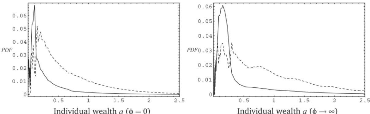
Figure2 shows the stationary distribution of wealth for the two limiting cases φ→∞andφ=0differentiated with respect to the two occupational classes. In
gen-6Tables3and4only display selected cases, with perfect markets(φ→∞), no credit markets(φ=0)
and the case, where the lower bound for the equity–loan–ratio is one half of the operating capital (φ=1). The upper limit is approximated withφ=1000in our numerical simulations. Figures4,6, and7cover a wider range of values forφfrom our simulations.
7Throughout the discussion of results we will refer to ‘optimal’ levels as those of the unconstrained
0.5 1 1.5 2 2.5 0 0.01 0.02 0.03 0.04 0.05 PDF
(a) Individual wealtha
-12 -10 -8 -6 -4 -2 0 0 0.01 0.02 0.03 0.04 0.05 PDF
(b) Log of individual wealthln(a)
Figure 1: Wealth distribution in the baseline model,φ→∞(dashed) andφ=0(solid)
0.5 1 1.5 2 2.5 0 0.01 0.02 0.03 0.04 0.05 0.06 Individual wealtha(φ=0) PDF 0.5 1 1.5 2 2.5 0 0.01 0.02 0.03 0.04 0.05 0.06 PDF Individual wealtha(φ→∞)
Figure 2: Wealth distribution in the baseline model for workers (solid) and entre-preneurs (dashed) withφ→∞andφ=0
eral, our model produces wealth distributions similar to those reported in the liter-ature for heterogeneous agent models with entrepreneurial activity (seeQuadrini,
1999,2000;Cagetti and De Nardi,2006a). We observe that workers are more con-centrated at lower wealth levels, and there exists a significant mass of wealthy en-trepreneurs but also a comparably large share of poorer ones. This is in line with empirical findings byGentry and Hubbard(2004);Hamilton(2000) as well as with related theoretical contributions (cf. Bohá˘cek, 2006, 2007). Relaxing credit con-straints significantly increases the mass of entrepreneurs in the upper tail of the distribution, but also leads towards an outward shift of the worker PDF of wealth, increasing mean and modal worker wealth levels.
Figure 3 shows the cumulative distribution of firm sizes in the intermediate goods sector for three distinct values of the parameterφwhich indicates the tight-ness of financial constraints. Each entrepreneur is able to operate his busitight-ness at the optimal firm size (8) in the perfect market case(φ→∞). Consequently, we observe
-5 -4 -3 -2 -1 0 1 2 0 0.2 0.4 0.6 0.8 1
Firm sizek(logarithmic scale)
CDF(k)
Figure 3: CDF of firm size in the baseline model with φ→∞ (dashed), φ=1.0
(dotted) andφ=0(solid)
a stepwise CDF, each step corresponding to the optimal firm size associated with one out of the five underlying possible productivity statesθe,h.
Consider next the caseφ=1, where entrepreneurs are able to acquire external financing up to maximum sum equal to their own wealth. Here, the operating firm size is bounded from above to twice the amount of individual wealth, which need not be the optimal firm size, especially, if the firm owner is highly productive. Recall at this point that the optimal firm size is endogenously determined; besides idiosyncratic random productivity also depending on factor prices, which in turn are determined by aggregate market activities and occupational choice in the general equilibrium.
The first observation is that the optimal firm sizes rise slightly for each possible state of entrepreneurial talentθe,h. This increase in firm sizes can be ascribed to the factor price effect. Borrowing constraints prevent the efficient allocation of capital among sectors such that too much capital is employed in the production of the final good. This is associated with a decline in the real interest rate, which in turn raises the optimal firm size in the intermediate sector for each state of productivity.
The second, major observation in the credit–constrained economy is that there is a positive mass of entrepreneurs between each two subsequent steps of optimal firm sizes, and the distribution is more concentrated at smaller firm sizes. Constraints become binding for many entrepreneurs, who now have to operate their enterprise at a suboptimally low scale. Non–surprisingly, this effect is aggravated, if we reduce the availability of external financing to naught. Forφ=0, steps in the CDF almost vanish, which means that more business owners are subject to constraints. The
Table 3: Simulation results — baseline model and modified credit constraint
Tightness of constraints
φ→∞ φ=1.0 φ=0
baseline model modified constraint
entrepreneurship rate (%) 0.230 0.247 0.243 0.250
∅firm size total 0.652 0.440 0.504 0.296
∅credit rationing total 0.000 0.330 0.205 0.637
∅profits total 0.134 0.124 0.130 0.114 final Y 0.147 0.130 0.139 0.111 goods KF(%) 0.438 0.521 0.492 0.612 sector KF 0.116 0.118 0.119 0.116 LF 0.820 0.796 0.805 0.786 factor w 0.113 0.103 0.109 0.089 prices r 0.028 0.017 0.022 0.007 w/(r+δ) 1.277 1.337 1.326 1.335 factor labor 0.630 0.630 0.630 0.630 income capital 0.160 0.134 0.142 0.114 shares profits 0.210 0.236 0.228 0.256 ∅wealth total 0.266 0.227 0.241 0.190 workers 0.203 0.167 0.180 0.128 entrepreneurs 0.477 0.410 0.431 0.378 ∅income workers 0.138 0.121 0.131 0.102 entrepreneurs 0.176 0.156 0.166 0.139 risk premium 0.118 0.141 0.126 0.218 ∅consumption 0.131 0.117 0.125 0.100 welfare -8.024 -8.966 -8.397 -10.504 wealth total 0.559 0.556 0.557 0.599 inequality workers 0.506 0.528 0.511 0.588 (Gini) entrepreneurs 0.546 0.488 0.525 0.478 mobility 0.143 0.154 0.152 0.156
optimal levels of firm sizes for the different states of productivity rise even further, due to the factor price effect. In numbers, if we compare the unconstrained with the completely constrained economy, businesses in the entrepreneurial sector on average operate at 32% of their respective optimal firm size.
Macroeconomic effects Table3and Figure4summarize the results for the macroe-conomic key variables of the calibrated baseline model. The general picture reflects the outcome one would expect from credit market improvements. Aggregate output
Y, consumption, aggregate wealth holdingsa, factor pricesr,wand incomes as well as welfare increase if we relax borrowing constraints.
2 4 6 8 10 0.3 0.4 0.5 0.6 0.7 0.8 0.9 1 φ
(a) % of optimal average firmsize
2 4 6 8 10 0.23 0.235 0.24 0.245 0.25 φ (b) Entrepreneurship rate 2 4 6 8 10 0.8 0.85 0.9 0.95 1 φ (c)Y relative toφ→∞ 2 4 6 8 10 -10.5 -10 -9.5 -9 -8.5 -8 φ (d) Welfare 2 4 6 8 10 0.19 0.2 0.21 0.22 0.23 0.24 0.25 0.26 φ (e) Wealth holdings
2 4 6 8 10 0.55 0.56 0.57 0.58 0.59 0.6 φ
(f) Gini of total wealth
2 4 6 8 10 0.2 0.3 0.4 0.5 0.6 φ labor capital profit
(g) Functional distribution of income
2 4 6 8 10 0.04 0.06 0.08 0.1 0.12 0.14 0.16 0.008 0.012 0.016 0.02 0.024 0.028 φ w(left scale) r(right scale) (h) Factor prices Figure 4: Macroeconomic effects of a change inφ, baseline model
2 4 6 8 10 0.12 0.14 0.16 0.18 0.2 0.22 φ
(i) Risk premium on entrepreneurial activity
2 4 6 8 10 0.144 0.146 0.148 0.15 0.152 0.154 0.156 φ (j) Mobility (% of population)
Figure 4: Macroeconomic effects of a change inφ, baseline model (cont.)
Figure4shows that, except for wealth inequality (which we will refer to later), the response of the macroeconomic variables to a change inφis monotonous. The overall loss in output of a perfectly constrained compared to a frictionless economy lies at about 25%, and wealth holdings only make up to 72% of their optimal level. Increasing financial constraints goes along with a substantial drop in economic per-formance. Average consumption declines by 24% and the associated welfare loss of the simulated model amounts to 30%.
We also see from Figure4that the response of output, wealth, factor prices, and welfare to a change inφis concave. The marginal gains of improving credit markets are much higher for small values ofφ, especially in the range of loan–to–equity ratios from0<φ<2, which is the empirically plausible domain. This interval accounts for more than two–thirds of the overall output loss associated with financial constraints. Given the general equilibrium nature of the underlying model, one would expect several adjustments to take place following a reduction in external financing as borrowing constraints become more tight. If there is only limited or no capital demand from the intermediate goods industry, we observe a capital–relocation effect between sectors. More capital is employed in the final goods industry. This amounts to shifting about 17% of the aggregate capital stock from the intermediate to the final goods sector over the entire range0φ<∞. The average excess demand for capital in the intermediate goods industry amounts to more than twice the average firm size.
With diminishing marginal returns, the equilibrium interest rate r, and accord-ingly the factor price for capitalr+δ, decline in both sectors of the economy. Recall-ing that entrepreneurial households receive income from two sources, profits and capital incomes, the income share reflecting the user costs of capital declines for any given level of individual wealth, whereas the profit share rises. Altogether, we
observe a shift in the functional income distribution from capital to profit incomes of 4.6 p.p. over the entire domain ofφ.8 The additional employment of capital c.p. raises labor productivity. The factor–price ratiow/(r+δ) increases, but only by a small scale of 4.4%, because this effect is partly offset by a reduction in intermediate good inputs, the latter reducing labor productivity.
The presence of credit constraints not necessarily implies that only those agents choose to become an entrepreneur, who have sufficient own wealth and borrowed resources to operate their business at the optimal firm sizek∗. These are the only firms which actually maximize their profits, whereas the constrained entrepreneurs are forced to operate at suboptimally small business sizes. Consequently, the aver-age firm size in the intermediate goods industry decreases substantially as financial constraints become more tight, and highly productive entrepreneurs are more af-fected by the constraints than those with a lowθe. Figure4a shows that in a com-pletely constrained economy the average firm size only amounts to around 32% of its optimal size.
Most strikingly, this result is also partly due to the fact that the entrepreneurship rate increases by almost 2 p.p. for smaller values ofφ. Instead of less competition in the intermediate goods industry, as one might have expected, we observe an increase in the number of firms in the constrained economy. This, however, comes at the cost of smaller market shares and lower average profits (–15%).
A higher rate of entrepreneurship as a consequence of tightening borrowing constraints is to some extent a counter–intuitive result and can be traced back to the general equilibrium nature of our approach. Credit constraints are only one out of several determinants of occupational choice. The competition for capital between the final and intermediate goods sector determines the equilibrium interest rate, the firm size and expected profits of the monopolistic enterprises. The expected premium of entrepreneurial incomes over wages, too, affects the individual decision on the future occupation. Figure 4i shows that the expected income differential attains its largest value in the perfectly constrained economy, then dropping sharply by more than 46% for an increase inφ.
Households continuously decide between two lotteries and possess (at least sub-jective) knowledge regarding the stochastic properties of the underlying shocks. If shocks are serially correlated, a low–productivity worker is aware of the fact that being also lowly productive in the future is a more probable outcome than other-wise. Consequently, he might be inclined to take his chances with entrepreneurship, knowing that his current productivity as a worker is not related to his future pro-ductivity as a business owner.9
8See2.4for a short remark on the equilibrium factor shares of the frictionless economy.
9Relaxing this assumption is left for future research; see alsoCagetti and De Nardi(2006a,
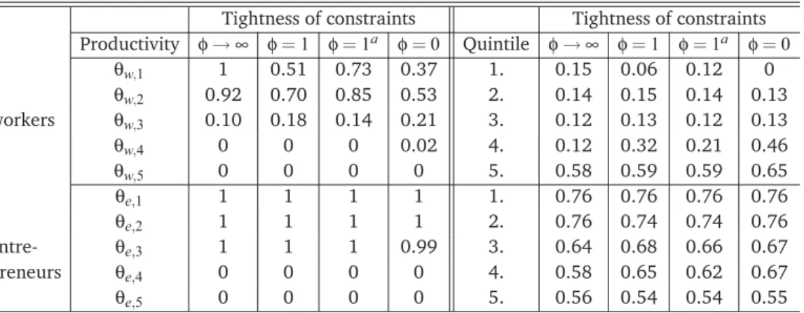
Table 4: Mobility in the baseline model: Individual probability of a switch in occupations with respect to current productivity state and wealth quintile
Tightness of constraints Tightness of constraints Productivity φ→∞ φ=1 φ=1a φ=0 Quintile φ→∞ φ=1 φ=1a φ=0 θw,1 1 0.51 0.73 0.37 1. 0.15 0.06 0.12 0 θw,2 0.92 0.70 0.85 0.53 2. 0.14 0.15 0.14 0.13 workers θw,3 0.10 0.18 0.14 0.21 3. 0.12 0.13 0.12 0.13 θw,4 0 0 0 0.02 4. 0.12 0.32 0.21 0.46 θw,5 0 0 0 0 5. 0.58 0.59 0.59 0.65 θe,1 1 1 1 1 1. 0.76 0.76 0.76 0.76 θe,2 1 1 1 1 2. 0.76 0.74 0.74 0.76 entre- θe,3 1 1 1 0.99 3. 0.64 0.68 0.66 0.67 preneurs θe,4 0 0 0 0 4. 0.58 0.65 0.62 0.67 θe,5 0 0 0 0 5. 0.56 0.54 0.54 0.55
aColumn depicts probabilities of the model with modified constraints, see Section4.2.
Regarding the wealth distribution, we first observe a sharp decline in the Gini coefficient for a rise in φ from 0.60 to 0.54, which is then followed by a gradual increase in overall wealth inequality back to a value of 0.56. This non–monotonic behavior of total wealth inequality can be explained, if we look at the within–group inequality for workers and entrepreneurs respectively. Table3shows that wealth be-comes more unevenly distributed among workers, whereas wealth inequality among entrepreneurs declines.10
Mobility Next, we are interested in the mobility between occupations taking place under the stationary distribution. Table3 and Figure4jshow that around 15% of the population switch between occupations in each period. We even observe over-all mobility to increase by 8% if credit constraints become more tight. While this change in overall mobility might seem small from a quantitative perspective, it is nevertheless remarkable, since it indicates that credit constraints not only increase the entrepreneurship rate of the economy but also the fluctuation between occupa-tions.
Table 4presents the quantitative results for each of the five productivity states θe,h,θw,h and with respect to wealth quintiles. A more detailed look at the mobility patterns shown in Table 4 reveals that generally workers and entrepreneurs who exhibit a low productivity (θ1−θ3) in their current profession decide to switch
be-tween professions, whereas the high productivity individuals (θ4,θ5) stay put. For
instance, all workers in the unconstrained economy, who currently are in the low-est labor productivity state, decide to take their chances with entrepreneurship in
10Notice, that the Gini coefficient does not allow for a simple decomposition of total inequality into
the next period. However, the probability of status change responds sensitive to the degree of credit availability. For φ=0, the probability drops down by almost two–thirds. As a general result we find that the likelihood of workers to start a busi-ness and become self–employed in the next period decreases in productivity and in constrained access to external financing. More productive workers show a larger persistence in their present occupation.
Regarding mobility, the picture is even more striking for individuals, who cur-rently are low productivity entrepreneurs. (Almost) All entrepreneurs finding them-selves in the lowest three productivity states change their occupation. They, (almost) with certainty will exit the market to seek employment as a worker in the next pe-riod. This results holds irrespective of the degree of constraint. Summing up, mo-bility over occupations in our model is confined to agents who are not successful in their current professions.
The intuition is as outlined before: Serially correlated shocks provide agents with a signal regarding future productivity. Since we assumed the processes for labor efficiency and entrepreneurial ability to be uncorrelated, a worker can infer from a low productivity today a probably low labor efficiency tomorrow, but this not necessarily indicates a equally low future ability as entrepreneur, which is given by the unconditional probability of states.
Table 4 also shows how the mobility over occupations depends on individual wealth. Conditional on the given occupation and the tightness of credit constraints, the values in the table represent the probability for a change of occupation for each quintile of the wealth distribution. As can be seen, the probability for a worker to become an entrepreneur increases in wealth, whereas the opposite is true for entrepreneurs. The general mobility pattern is robust over different levels ofφ. The result is, however, not quite surprising given the fact that agents are risk averse and that profit income is more risky than labor income.
While the effects of credit constraints on the mobility patterns for entrepreneurs are only small in scale, we observe significant effects on mobility patterns for work-ers. More tight credit constraints strikingly decrease the probabilities of becoming an entrepreneur for poor workers, while the corresponding probabilities for rich workers (especially for those in the fourth quintile) increase. New entrepreneurs are mainly recruited among the group of wealthy workers.
4.2 An Alternative Formulation of Borrowing Constraints
The borrowing of the baseline model were assumed to be entirely related to in-dividual wealth. We will now discuss a separate treatment, where the maximum loan also depends on the entrepreneur’s individual productivity. In case of de-fault, the lender is able to seize the fraction φ of the borrower’s gross income
-5 -4 -3 -2 -1 0 1 2 0 0.2 0.4 0.6 0.8 1
Firm sizek (logarithmic scale)
CDF(k)
Figure 5: CDF of firm size withφ=1for the baseline model (solid) and the model with modified credit constraint (dashed)
constraint making sure that it is never optimal for the borrower of going into default becomes:
π(θ(i)e,a(i) +b(i)) + (1+r)a(i)(1−φ)[π(θ(i)e,a(i) +b(i)) + (1+r)a(i)] + (1+r)b(i)
⇐⇒ ba((ii)) ≤φ+φπ(θ((i)e,a(i) +b(i))
1+r)a(i) (15)
The upper bound for the debt–to–equity ratio now also depends on the entrepren-eur’s profitability. It increases with a higher realization θ(i)e of the idiosyncratic productivity shock.
Figure5shows the resulting cumulative distribution function of firmsizes for the modified model and compares it with the baseline setting for the case ofφ=1. A comparison between eqs. (9) and (15) shows that including profit incomes into the collateral raises the debt–to–equity ratio by the amount of the second term on the RHS of equation (15).
Obviously, the model modification does not alter the general picture of how fi-nancial constraints affect the size distribution of firms. We observe a greater number of larger firms. The optimal firm sizes (indicated by the steps in the CDF) decrease slightly for each state of entrepreneurial talent θe,h. This, again, can be explained with the factor price effect. If being more productive compensates for a lack of wealth, we expect the overall credit supply to the intermediate goods industry to be larger than in the baseline model. Less capital is employed in the final good sector, and the real interest rate rises. The larger user cost of capital explain the decrease in the optimal firm size in the noncorporate sector for each state of productivity.
2 4 6 8 10 0.3 0.4 0.5 0.6 0.7 0.8 0.9 1 φ
(a) % of optimal firmsize
2 4 6 8 10 0.23 0.235 0.24 0.245 0.25 φ (b) entrepreneurship rate 2 4 6 8 10 0.8 0.85 0.9 0.95 1 φ (c)Y relative toφ→∞ 2 4 6 8 10 -10.5 -10 -9.5 -9 -8.5 -8 φ (d) welfare 2 4 6 8 10 0.55 0.56 0.57 0.58 0.59 0.6 φ
(e) Gini of total wealth
2 4 6 8 10 0.144 0.146 0.148 0.15 0.152 0.154 0.156 φ (f) mobility 2 4 6 8 10 0.12 0.14 0.16 0.18 0.2 0.22 φ (g) risk premium
Figure 6: Properties of the model with modified credit constraint (solid) for differ-ent levels ofφcompared to the baseline model (dashed)
The last column of Table3presents the results from the numerical simulation of the modified model forφ=1. Naturally, there should be no differences in results for the two limiting cases of perfect (φ→∞) or no credit market (φ=0) respectively. Figure6compares the baseline to the modified setting. We find the major results of our analysis preserved.
The significant effect is one in magnitude. Compared to the baseline model, the maximum loan is positively related to individual entrepreneurial productivity, which is effective for any given value of0<φ<∞. This constitutes a credit market improvement, because now also relatively poor but highly productive agents are el-igible for external financing. If we consider the case ofφ=1, the loss in aggregate output compared to the perfect market scenario now only amounts to 5%, versus 11.5% of the baseline model. Qualitatively similar results can be observed for aver-age wealth, individual incomes, consumption and factor prices, which exceed their corresponding values of the baseline economy. Wealth inequality is slightly larger under the modified borrowing constraint, which can mainly be ascribed to a more uneven distribution among firm owners.
The fraction of capital employed in the intermediate goods industry increases by roughly 3 p.p. Except for very small values of φ, the entrepreneurship rate of the modified model is smaller than in the baseline economy (see the above mentioned general equilibrium effects), but average firm sizes and profits are larger. The aver-age firm size attains around 77% (vs. 67%) of its respective optimal value, and the average excess demand for capital in the intermediate goods industry only amounts to 40% (vs. 75%) of average business size.
Altogether, we observe that the economy, where the maximum loan also depends on individual productivity, responds more sensitive to changes in φ, the marginal gains of relaxing borrowing constraints being larger than in the baseline model.
Regarding mobility, we also find results qualitatively similar to the original model. Mobility is decreasing if borrowing constraints are relaxed, and—except for very small values ofφ—the overall mobility between occupations is lower under the modified borrowing constraint. Table4shows how the probabilities of switch-ing between occupations with respect to productivity states and wealth quintiles are affected, if credit availability also depends on individual productivity. The proba-bility of switching occupations is higher for workers of the two lowest productivity states (θw,1,θw,2) over the entire range ofφ, which follows directly from (15), where
productivity unambiguously has a positive effect on the debt–to–equity ratio. Those entrepreneurs, who are members of the third and fourth quintile are less likely to switch, which reflects that ability compensates for lack of wealth.
Table 5: Simulation results withiidshocks
Tightness of constraints φ→∞ φ=1.0 φ=0
entrepreneurship rate (%) 0.245 0.244 0.240
∅firm size total 0.376 0.355 0.327
∅credit rationing total 0.000 0.045 0.129
∅profits total 0.093 0.093 0.094 final Y 0.108 0.105 0.100 goods KF (%) 0.438 0.456 0.489 sector KF 0.072 0.073 0.075 LF 0.758 0.759 0.763 factor w 0.090 0.087 0.082 prices r 0.045 0.041 0.033 w/(r+δ) 0.849 0.861 0.887 factor labor 0.630 0.630 0.630 income capital 0.160 0.154 0.143 shares profits 0.210 0.216 0.227 ∅wealth total 0.164 0.159 0.154 workers 0.054 0.053 0.039 entrepreneurs 0.502 0.450 0.517 ∅income workers 0.096 0.093 0.086 entrepreneurs 0.146 0.143 0.142 risk premium 0.030 0.065 0.140 ∅consumption 0.098 0.095 0.091 welfare -10.420 -10.713 -11.336 wealth total 0.637 0.631 0.676 inequality workers 0.323 0.362 0.414 (Gini) entrepreneurs 0.379 0.311 0.246 mobility 0.025 0.014 0.004
4.3 The Model withIIDShocks
Although income and earnings persistence is the relevant environment from an em-pirical point of view, we now confront the results from the baseline model with the case ofiidshocks. The major purpose of this exercise is to demonstrate how sensi-tive the model responds to a change in serial correlation, especially, if it comes to the implications for occupational choice and social mobility.
Table5shows the results from our numerical simulations, and Figure7compares the baseline setting to the model withiidshocks. We observe that the qualitative re-sults for aggregate output, wealth holdings, factor prices, consumption, and welfare closely resemble the baseline model, although the effects differ in magnitude.