QUANTITATIVE FINANCE RESEARCH CENTRE QUANTITATIVE F
INANCE RESEARCH CENTRE
Q
UANTITATIVE
F
INANCE
R
ESEARCH
C
ENTRE
Research Paper 255
Modelling the Evolution of Credit Spreads using the Cox
process within the HJM framework: a CDS Option Pricing Model
Carl Chiarella, Viviana Fanelli and Silvana Musti
ISSN 1441-8010 www.qfrc.uts.edu.au
Modelling the Evolution of Credit Spreads using the
Cox process within the HJM framework: a CDS
Option Pricing Model
Carl Chiarella
∗Viviana Fanelli
†Silvana Musti
‡Abstract
In this paper a simulation approach for defaultable yield curves is developed within the Heath et al. (1992) framework. The default event is modelled using the Cox pro-cess where the stochastic intensity represents the credit spread. The forward credit spread volatility function is affected by the entire credit spread term structure. The paper provides the defaultable bond and credit default swap option price in a proba-bility setting equipped with a subfiltration structure. The Euler-Maruyama stochastic integral approximation and the Monte Carlo method are applied to develop a numer-ical algorithm for pricing. Finally, the Antithetic Variable technique is used to reduce the variance of credit default swap option prices.
Keywords: Pricing, HJM model, Cox process, Monte Carlo method, CDS option
JEL Classification: C63, G13, G33
∗School of Finance and Economics, University of Technology, Sydney, PO Box 123, Broadway, NSW
2007, Australia ([email protected])
†Corresponding Author: Dipartimento di Scienze Economiche, Matematiche e Statistiche, Università
degli Studi di Foggia, Largo Papa Giovanni Paolo II, 1, 71100, Foggia, Italy ([email protected])
‡Dipartimento di Scienze Economiche, Matematiche e Statistiche, Università degli Studi di Foggia,
1
Introduction
Since the 1990s, the focus on credit risk has increased amongst academics and financial market practitioners. This is due to the concerns of regulatory agencies and investors regarding the high exposure of financial institutions to over-the-counter derivatives. It is also due to the rapid development of markets for price-sensitive and credit-sensitive instruments that allow institutions and investors to trade this risk.
The New Basel Accord (International Convergence of Capital Measurement and Capital Standard, Basel II, 26 January 2004) promotes the standards for credit risk management, obligating financial institutions to fulfill a variety of regulatory capital requirements. By increasing the reliability of the credit derivative market, the Basel II rules have contributed to its success.
In the credit risk literature two principal kinds of models are widely used: the structural models and the reduced form models.
Structural models were proposed by Merton (1974), Black and Cox (1976), Shimko et al. (1993) and Longstaff and Schwartz (1995), to cite the principal contributions. These models focus on the analysis of a firm’s structural variables: the default event derives from the evolution of the firm’s assets and it is completely specified in an endogenous way.
The main drawback of the structural approach is that since many of the firm’s assets are typically not traded, the firm’s value process is fundamentally unobservable, making implementation difficult. Furthermore, this approach assumes that only bonds with ho-mogeneous levels of seniority exist and that the risk-free rates are constant over the period of evaluation.
Zhou (1997) and Schönbucher (1996) are two important contributions that use jump diffusion processes for the evolution of the firm’s value in the Merton model. These models are more realistic in generating the shape of a credit spread term structure compared to the classical structural models that seem to underestimate credit spread values. Jump-diffusion models also have the advantage of allowing the default event to occur abruptly.
Reduced form models are characterized by a more flexible approach to credit risk. They mainly model the spread between the defaultable interest rate and the risk-free rate. The default time is a stochastic variable modelled as a stopping time. The two earliest contributions to this approach are those of Jarrow and Turnbull (1995) and Jarrow et al. (1997).
Jarrow and Turnbull (1995) consider a constant and deterministic Poisson intensity. In contrast, Jarrow et al. (1997) consider the issuer’s rating as the fundamental variable driving the default process and the rating dynamics are modelled as a Markov chain, where default is the absorbing state.
Lando (1998) uses a stochastic intensity, while the default process is described by a Cox process which allows a remarkable degree of analytical tractability. The Cox process is a generalization of the Poisson process when the intensity is random. If the Cox process is conditional on a particular realization of the intensity, it becomes an inhomogeneous Poisson process.
Das and Sundaram (2000) find a more flexible pricing methodology valid both for bonds and credit derivatives. A defaultable bond price is equal to the expected value of future payoffs discounted by a defaultable interest rate. The term structure models existing in the literature, such as Cox et al. (1985) and Heath et al. (1992) can then be used to model
the defaultable term structure.
An important result demonstrated in Duffie and Lando (2001) is the way in which a structural model of the Black and Cox (1976) type is consistent with the reduced form class of models when asymmetric information about structural characteristics are revealed.
Recently, academics and practitioners have utilized the risk-neutral pricing methodol-ogy to carry out credit spread term structure analysis. Duffie and Singleton (1999) provide a discrete-time reduced-form model in order to evaluate risky debt and credit derivatives in an arbitrage-free environment. They add a forward spread process to the forward risk-free rate process and use the Heath et al. (1992) approach to obtain the arbitrage-free drift restriction and by using the "Recovery of Market Value" condition (Duffie and Singleton (1999)), they provide a recursive formula that is easy to implement.
The HJM approach is used by Schönbucher (1998) in order to model the term structure of defaultable interest rates. The defaultable bond price is obtained under the following assumptions: i) positive recovery rates, ii) reorganization of the defaulted firms with the possibility of multiple default, and iii) uncertainty about the magnitude of the default. Furthermore, the firm’s default causes jumps in the defaultable interest rate process. Using the HJM approach, Schönbucher (1998) provides a drift restriction for the defaultable term structure. A similar result is obtained in Pugachevsky (1999), where the HJM drift restriction is obtained by applying the arbitrage free condition obtained in Maksyumiuk and G¸atarek (1999) and without assuming any jumps to default.
Finally, Jeanblanc and Rutkowski (2002), Jamshidian (2004) and Brigo and Morini (2005) suggest a different approach to defaultable bond and credit derivative modelling: in a probability space equipped with a subfiltration structure the default is modelled as a Cox process. Furthermore, Chen et al. (2008) provide a model for valuing a credit default swap when the interest rate and the hazard rate are correlated. They provide an explicit solution to the model by solving a bivariate Riccati equation. Their model is solved quickly so that all the parameters of the model are simultaneously estimated.
In this paper, we build on the cited recent literature and develop a model for credit spread term structure evolution and credit derivative pricing. The HJM model has been extensively analyzed in the literature from a theoretical point of view: our intent, instead, is to focus on the applications of the model for pricing technique purposes. In particular, we model the forward credit spread curve within the HJM framework using the theory of Cox processes where the stochastic intensity represents the credit spread. The HJM model is known to be one of the most general term structure models and for this reason we have chosen to extend its interest rate dynamics to the defaultable rate: the forward credit spread volatility function, the initial credit spread curve and specifications of the volatility structure are the sole inputs. Because of the arbitrage-free condition, the drift can be expressed in terms of the volatility. We assume a stochastic volatility for both the risk-free interest rate and the credit spread, so that analytical results are not readily available and model implementation is generally possible only via a numerical simulation approach. We develop and implement an efficient numerical algorithm that allows bond and credit derivative pricing. The accuracy of the calculated values is improved by the application of a well known method of variance reduction, the Antithetic Variable technique.
In Section 2 we describe the model. In Section 3 we outline the foundations of credit default swap (CDS) pricing and derive CDS option pricing formulae under the equivalent martingale measure. In Section 4 we outline the application of Monte Carlo simulation to
the HJM model based on the Euler-Maruyama discretisation of the forward rate dynam-ics. A variance reduction technique is applied to improve the efficiency of the Monte Carlo method and to provide more accurate numerical results for pricing. Then, the efficiency of the algorithm in terms of runtimes is investigated. The analysis concerning the run-time/accuracy trade-off indicates how the algorithm can be successfully utilized by credit risk practitioners in order to price credit risk products with satisfactory levels of accuracy and reasonable runtimes. Section 5 concludes.
2
Model setting
The model is set in a filtered probability space (Ω,F,(Ft)t≥0,P), T is assumed to be the finite time horizon andF =FT is theσ-algebra at time T. All statements and definitions are understood to be valid until the time horizonT. The probability space is assumed to be large enough to support both an Rd-valued stochastic process X ={X
t : 0≤t ≤T} that
is right continuous with left limit, and a Poisson processN(t)with N(0) = 0, independent of X.
The background driving process X generates the subfiltration H= (Ht)t≥0 = (σ(Xs : 0≤s≤t))t≥0 representing the flow of all background information except default itself and
H=HT is the sub-σ-algebra at timeT.
The Poisson process N(t) has a non negative and right-continuous stochastic intensity
λ(t) which is independent of N(t)and follows the diffusion process
dλ(t) = µλ(t)dt+σλ(t)dWλ(t), (1)
where µλ(t) is the drift of the intensity process, σλ(t) is the volatility of the intensity
process and Wλ is a standard Wiener process under the objective probability measure P.
The intensity process λ(t) is assumed to be adapted to H, and the assumption of time dependent intensity implies the existence of an inhomogeneous Poisson process.
In the subfiltration setting outlined above it is natural to consider an Ht-conditional
Poisson process in such a way that a Cox process is associated with the state variables process X and the intensity function λ(t). We define τi, i ∈ N, as the times of default
generated by the Cox process N(t) = P∞i=11{τi≤t} with intensity λ(t). In this paper we
only consider the time of the first default and it will be referred to with τ :=τ1. Then, the defaultable time τ is a stopping time, τ : Ω→R+
0, defined as the first jump time of N(t),
τ =inf{t ∈R+0|N(t)>0}.
The right-continuous default indicator process 1{τ≤t} generates the subfiltration Fτ =
(Fτ
t)t≥0 = (σ(1{τ≤s} : 0 ≤ s ≤ t))t≥0, that is assumed to be one component of the full filtration F = (Ft)t≥0. Since obviously Ftτ ⊂ Ft, ∀t ∈ R+0, τ is a stopping time with respect to F, but it is not necessarily a stopping time with respect to H. It follows that F=H∨Fτ, that is F
t=Ht∨Ftτ ∀t ∈R+0.
For any t ∈ R+0, we define the default probability as P(τ ≤ t|Ht) and the survival
probability as P(τ > t|Ht). These two quantities indicate, respectively, the probability of
default occurring or not occurring up to time t. In the subfiltration setting, asset pricing is consistent with the application of the iterated expectation law.
At any time t, the risk-free zero-coupon bond price is denoted by P(t, T), where T
represents the maturity time, T > t, and it is calculated according to
P(t, T) =e−RtTf(t,s)ds, (2)
where f(t, T) is the instantaneous risk free forward rate at time t applicable at fixed maturity T. Conversely, if the derivative of P(t, T) with respect to maturity T exists, the instantaneous risk free forward rate can be written in terms of the bond price as
f(t, T) = − ∂
∂TlogP(t, T). (3)
We assume that the forward rate is driven by the diffusion process
df(t, T) = α(t, T,·)dt+σ(t, T,·)dW(t), (4) where α(t, T,·) is the instantaneous forward rate drift function, σ(t, T,·) is the instanta-neous forward rate volatility function and W(t)is a standard Wiener process with respect to the objective probability measure P. The third argument in the brackets (t, T,·) indi-cates the possible forward rate dependence on other path dependent quantities, such as the spot rate or the forward rate itself. The instantaneous risk-free short rate r(t) is defined as r(t) :=f(t, t).
We recall that the HJM no-arbitrage drift restriction is
α(t, T,·) = σ(t, T,·) ·Z T t σ(t, s,·)ds−φ(t) ¸ . (5)
Similar statements hold for defaultable bonds. We indicate with Pd,R(t, T) the generic
price at any time t of a defaultable zero-coupon bond with maturity T and recovery rate
R. If we set Pd(t, T) := Pd,0(t, T), we have Pd(t, T) =1{τ >t}e− RT t fd(t,s)ds, (6)
where fd(t, T) is the instantaneous defaultable forward rate at time t applicable to fixed
maturity T. If the derivative of Pd(t, T) with respect to maturity T exists and assuming
that the default occurs after t, the instantaneous defaultable forward rate can be written in terms of the bond price as
fd(t, T) =−
∂
∂TlogPd(t, T) (7)
and is assumed to be modelled by the stochastic process
dfd(t, T) =αd(t, T,·)dt+σd(t, T,·)dWd(t), (8)
where αd(t, T,·) and σd(t, T,·) are, respectively, the drift function and the volatility
func-tion of the instantaneous defaultable forward rate. FurthermoreWd(t)is a standard Wiener
process with respect to the objective probability measureP. As in (4), the third argument in the brackets (t, T,·) indicates, again, the possible defaultable forward rate dependence
on other path dependent quantities, such as the defaultable spot rate or the defaultable forward rate itself.
Spot rate dynamics are derived from the forward rate dynamics, since rd(t) :=fd(t, t).
Recalling that the market is arbitrage free if and only if there exists a probability measure
e
Psuch that discounted asset price processes are martingales, the defaultable bond price is now obtained as the risk-neutral expectation of the discounted bond value, namely
Pd(t, T) = 1{τ >t}EPe[e− RT
t rd(s)ds|H
t] (9)
where e−RtTrd(s)ds is the defaultable stochastic discount factor and Pe is the risk-neutral
equivalent probability measure.
Following Lando (1998), the pricing formula at time t for a defaultable zero coupon bond with maturity T is given by
Pd(t, T) =EPe[e− RT t r(s)ds1{τ >T}|Ft] = =EPe[EPe[e− RT t r(s)ds1{τ >T}|HT ∨ Fτ t]|Ft] = =EPe[e− RT t r(s)ds1 {τ >t}EPe[1{τ >T}|HT ∨ Ftτ]|Ft] = =1{τ >t}EPe[e− RT t (r(s)+λ(s))ds|Ft] = =1{τ >t}EPe[e− RT t (r(s)+λ(s))ds|Ht]. (10)
The last equation follows from the law of iterated expectations. Comparing equation (9) with equation (10), we see that the default free and defaultable instantaneous spot rate are related by
rd(t) = r(t) +λ(t), (11)
where λ(t) is the (stochastic) intensity rate. So the credit spread at the short end is λ(t). Equation (11) suggests writing the credit spread across rates of all maturities as λs(t, T)
so that
fd(t, T) =f(t, T) +λs(t, T). (12)
We assume for λs(t, T) the dynamics
λs(t, T) =λs(0, T) + Z t 0 αλ(s, T,·)ds+ Z t 0 σλ(s, T,·)dWλ(s), (13)
whereαλ(t, T,·)is the drift,σλ(t, T,·)is the volatility of the credit spread curves andWλ(t)
is a standard Wiener process under P. For (11) and (12) to be compatible at T = t we must have
λ(t) = λs(t, t). (14)
From (13) it follows that the stochastic integral equation for λ(t)may be written
λ(t) = λs(t, t) = λs(0, t) + Z t 0 αλ(s, t,·)ds+ Z t 0 σλ(s, t,·)dWλ(s), (15)
from which (the subscript 2 denotes partial derivative with respect to the second argument)
dλ(t) = · αλ(t, t,·) + Z t 0 αλ2(s, t,·)ds+ Z t 0 σλ2(s, t,·)dWλ(s) ¸ dt+ σλ(t, t,·)dWλ(t). (16)
Thus in order that (1) and (16) be compatible it must be the case that theµλ(t)andσλ(t)
in equation (1) are given by
µλ(t) = αλ(t, t,·) + Z t 0 αλ2(s, t,·)ds+ Z t 0 σλ2(s, t,·)dWλ(s), σλ(t) = σλ(t, t,·).
For simplicity of expression we shall assume stochastic differential equations driven by one Brownian motion for both the risk-free forward rate and the credit spread. We denote the correlation between the Brownian motionsdW and dWλ becomes a scalar coefficient as
ρ=corr(dW, dWλ). (17)
We use the Heath et al. (1992) approach to model the term structure of defaultable interest rates. The main advantages of the HJM model are that in the formulation of the spot rate process and bond price process the market price of interest rate risk drops out by being incorporated into the Wiener process under the risk neutral measure; the model is automatically calibrated to the initial yield curve and the drift term in the forward rate differential equation is a function of the volatility term. As result of the latter characteristic, the HJM model can be considered as a class of models, each one identified by the choice of a volatility function. Consequently, we need to give a specific functional form to the volatility term in order to obtain a specific HJM model. The main complication of this approach is that some volatility functions make the dynamics for r(t) and rd(t) path dependent,
in other words non-Markovian, and since the bond price dynamics depend on these, they also become non-Markovian making the model difficult to handle, both analytically and numerically.
Using the HJM approach, we show in Appendix B that the no-arbitrage restriction on the drift of the credit spread process may be written as
αλ(t, T) =ρ · σ(t, T) Z T t σλ(t, s)ds+σλ(t, T) Z T t σ(t, s)ds ¸ dv +σλ(t, T) Z T t σλ(t, s)ds−σλ(t, T)φλ(t).
so that the stochastic dynamics for the defaultable forward rate, written in integral form, are fd(t, T) =f(0, T) +λs(0, T) +R0t h σ(v, T)RvT σ(v, s)ds+σλ(v, T) RT v σλ(v, s)ds i dv +R0tρ h σ(v, T)RvT σλ(v, s)ds+σλ(v, T) RT v σ(v, s)ds i dv +R0t h σ(v, T)dWf(v) +σλ(v, T)dWfλ(v) i . (18) In (18) f W(t) = W(t)− Z t 0 φ(s)ds, (19) f Wλ(t) = Wλ(t)− Z t 0 φλ(s)ds, (20)
are Wiener processes under the risk neutral measurePe and φ(t) andφλ(t)are respectively
the market prices of interest rate risk and credit spread risk. We consider a fairly general case of proportional volatility models. Following Chiarella et al. (2005) we consider a volatility function of the form
σ(t, T,·) =e−αf(T−t)[a
0+arr(t) +aff(t, T)]γ, γ >0 (21)
where r(t) is the spot interest rate and f(t, T) is the forward interest rate. Besides, we assume a credit spread stochastic volatility with the functional form
σλ(t, T,·) =e−αλ(T−t)[b0+b1λ(t) +b2λs(t, T)]γ, γ >0 (22)
where λ(t) is the spot credit spread and λs(t, T) is the forward credit spread. The factor
e−αλ(T−t) expresses the direct dependence of volatility on time to maturity. We have chosen to extend the functional form adopted for the risk-free forward rate to the spread volatility. Indeed, regression analysis applied to market data has shown a linear dependence of volatility both onλ(t) andλs(t, T), suggesting the coefficients that will be applied later
on (see equation (34) below) in the numerical implementation. We refer the reader to Fanelli (2007) for the volatility parameter analysis.
The result (10) can be extended to the case with non-zero recovery rate, defining the recovery rate R as the percentage of the par value at maturity refunded by the protection seller. We assume, as in Hull and White (2000, 2001), no systematic risk in recovery rates so that expected recovery rates, observed in the real world, are also expected recovery rates in the risk-neutral world. In the model implementation we use the recovery rate estimated by Moody’s (Moody’s Investors Service (2007)).
Applying properties of the Cox process and the law of iterated expectations, we calcu-late, under the equivalent martingale measure and in the case of positive recovery rate, R, the generic price at time t of a defaultable bond with maturity T according to
Pd,R(t, T) = EPe h e−RtTr(s)ds1 {τ >T}+Re− RT t r(s)ds1{τ≤T}|Ft i =EPe h e−RtTr(s)ds1 {τ >T}|Ft i +EPe h R(e−RtTr(s)ds(1−1 {τ >T})|Ft i =EPe h EPe h e−RtTr(s)ds1 {τ >T}|HT ∨ Ftτ i |Ft i +EPe h Re−RtTr(s)ds|F t i −EPe h EPe h Re−RtTr(s)ds1 {τ >T}|HT ∨ Ftτ i |Ft i =EPe h e−RtTr(s)ds1 {τ >t}EPe £ 1{τ >T}|HT ∨ Ftτ ¤ |Ft i +EPe h Re−RtTr(s)ds|F t i −EPe h e−RtTr(s)ds1 {τ >t}EPe £ R1{τ >T}|HT ∨ Ftτ ¤ |Ft i =1{τ >t}EPe h e−RtT(r(s)+λ(s))ds|H t i +EPe h Re−RtTr(s)ds|H t i −1{τ >t}EPe h Re−RtT(r(s)+λ(s))ds|H t i =RP(t, T) + (1−R)1{τ >t}EPe h e−RtT(r(s)+λ(s))ds|H t i . (23)
3
Credit default swap option
A credit default swap (CDS) is a contract between two parties, the protection buyer and the protection seller, which provides insurance against the default risk of a third party, called the reference entity. The protection buyer pays a periodic fee to the protection seller in exchange for a contingent payment upon a credit event occurring. Here we assume a CDS contract with maturityT for receiving protection against the default risk of a bond. This CDS is issued on an obligation with maturity T and allows a credit event payment (1-R) if the default occurs before time T, where R is the recovery rate, and τ < T is the default time.
Following Brigo and Morini (2005),S(t)is the rate calculated at timetrepresenting the amount paid by the protection buyer to the seller at every time Ti, i= 1, ..., n to receive
protection until timeTn. The time interval(Ti−Ti−1)represents the annual fraction. The buyer’s discounted payoff π(t, S(t)) att < T is
π(t, S(t)) = (1−R) n X i=1 D(t, Ti)1{Ti−1<τ≤Ti} | {z }
Floating or Contingent Leg
− n X i=1 D(t, Ti)(Ti−Ti−1)1{τ >Ti}S(t) | {z }
Fixed or Fee Leg
, (24)
where
D(t, T) =e−RtTr(s)ds (25)
is the discount factor on the interval[t, T]andr(t)is the risk-free spot interest rate. Under the risk neutral measure, the price at time t of a CDS with maturity T and rate S(t)is
CDS(t, S(t), T) =EPe[π(t, S(t))|Ft]. (26)
By substituting (24) into (26) and applying the properties of Cox processes and the iterated expected value law as already applied in the equation (10), we obtain
CDS(t, S(t), T) = n X i=1 EPe £ (1−R)D(t, Ti)1{Ti−1<τ≤Ti}|Ft ¤ − n X i=1 EPe £ D(t, Ti)(Ti−Ti−1)1{τ >Ti}S(t)|Ft ¤ (27) = n X i=1 EPe h EPe h (1−R)e−RtTir(s)ds(1 {τ >Ti−1}−1{τ >Ti})|HTi ∨ F τ t i Ft i − n X i=1 EPe £ EPe £ D(t, Ti)(Ti−Ti−1)1{τ >Ti}S(t)|HTi ∨ Ftτ ¤ Ft ¤ = n X i=1 1{τ >t}(1−R)EPe h e−RtTir(s)ds(e− RTi−1 t λ(s)ds −e− RTi t λ(s)ds)|F t i
− n X i=1 S(t)1{τ >t}EPe h e−RtTir(s)dse− RTi t λ(s)ds(T i−Ti−1)|Ft i = n X i=1 1{τ >t}(1−R)EPe h e−RtTir(s)ds(e− RTi−1 t λ(s)ds−e− RTi t λ(s)ds)|H t i − n X i=1 S(t)1{τ >t}EPe h e−RtTir(s)dse− RTi t λ(s)ds(T i −Ti−1)|Ht i = n X i=1 (1−R) n EPe h e−RtTir(s)dse− RTi−1 t λ(s)ds|H t i −Pd(t, Ti) o − n X i=1 S(t)(Ti−Ti−1)Pd(t, Ti). (28)
We calculate the fair rate S(t), called the par CDS spread, as the rate that sets the value of the CDS (28) to zero, thus
S(t) = (1−R) Pn i=1 n EPe h e−RtTir(s)dse− RTi−1 t λ(s)ds|Ht i −Pd(t, Ti) o Pn i=1(Ti−Ti−1)Pd(t, Ti) . (29)
Formula (29) may be approximated by (see Brigo and Morini (2005))
S(t) = (1−R) Pn iP=1{Pd(t, Ti−1)−Pd(t, Ti)} n i=1(Ti−Ti−1)Pd(t, Ti) . (30)
We now consider at timet a CDS option with maturity Ts and strike rate K issued on
a CDS which provides protection against default over the period [Ts, Tn=T], and denote
its value asCDSO(t, Ts, T). It has the discounted payoff given by
D(t, Ts)[CDS(Ts, K, T)]+ =D(t, Ts) CDS(Ts, K, T)−CDS(Ts, S(Ts), T) | {z } 0 + . (31)
By substituting (27) into (31), we obtain the discounted CDS option payoffχ(t, K)at time
t χ(t, K) =1{τ >Ts}D(t, Ts)× ×EPe £Pn i=s+1(Ti−Ti−1)D(Ts, Ti)1{τ >Ti}|HTs ¤ (S(Ts)−K)+. (32)
The CDS option price at time t is equal to the expected value of χ(t, K), conditional on Ft, CDSO(t, Ts, T) = EPe[χ(t, K)|Ft], = EPe " D(t, Ts)1{τ >Ts}EPe " n X i=s+1 (Ti−Ti−1)D(Ts, Ti)1{τ >Ti}|HTs # × ×(S(Ts)−K)+|Ft ¤ = 1{τ >t}EPe " D(t, Ts)1{τ >Ts} ( n X i=s+1 (Ti−Ti−1)Pd(Ts, Ti) ) (S(Ts)−K)+|Ht # . (33)
4
The numerical scheme
We consider the problem of a T-maturity zero coupon bond price evaluated at time t= 0, when only the initial forward curve is available. Such evaluation requires the simulation of the entire forward rate curve evolution under some volatility specification. As no analytical methods seem possible, we employ the Monte Carlo simulation method. We use a variance reduction procedure, in particular the Antithetic Variable (AV) technique, to improve numerical accuracy and reduce computational effort. We calculate the prices of all assets evaluated in this paper according to this technique and the last two columns of the Tables 1-6 in Appendix A show the numerical results. The basic task of the numerical algorithm we use is to simulate a possible evolution of the defaultable forward curve (18), fd(t, T),
over the time horizon[0, T], once given the initial forward curvefd(0, T), where 0≤t ≤T
and T ≤ T. The efficiency of the chosen numerical scheme has already been established for non-defaultable bond pricing in Chiarella et al. (2005), and it seems to provide an adequate technique to handle a non-Markovian evolution.
In the model implementation we use the iTraxx indices as credit spread values. The daily historical data is extracted from the Bloomberg provider. The period of reference is 21/03/2005-22/02/2007 and we consider the first series for 3 and 7-year maturity iTraxx indices and the third series for 5 and 10-year maturity iTraxx indices in order to have comparable daily data. By interpolating the index values relative to the various maturities, we obtain the initial spot credit spread curve.
Following Chiarella et al. (2005) we take the default free forward rate volatility function
σ(t, T, r(t), f(t, T)) =e−0.2(T−t)[0.016476−1.3353r(t) + 1.19843f(t, T)] and the spread volatility function
σλ(t, T, λ(t), λs(t, T)) =e−(T−t)[1.41494λ(t) + 0.61693λs(t, T)] (34)
based on the analysis of Fanelli (2007).
We divide [0, T] into N subintervals of length 4t = T
N, so that n = 4tt, m = 4Tt for 0 ≤ t ≤ T ≤ T and f(t, T) = f(n∆t, m∆t). The Euler-Maruyama discretisation is used to approximate the stochastic integral equation (18) (see Kloeden and Platen (1999)).
We start by considering at time zero the initial defaultable forward curve with generic maturity T = m∆t, where 1 ≤ m ≤ N, that is fd(0,0) = rd(0), fd(0,∆t), fd(0,2∆t),
...,fd(0, N∆t). Hence we obtain the generic recursive formula for the defaultable forward
curve evolution in the form
fd((n+ 1)∆t, m∆t) = f(n∆t, m∆t) +λ(n∆t, m∆t,·) +σ(n∆t, m∆t,·)Pmi=−n1σ(n∆t, i∆t,·)∆t+σλ(n∆t, m∆t,·) Pm−1 i=n σλ(n∆t, i∆t,·)∆t +ρ£σ(n∆t, m∆t,·)Pmi=−n1σλ(n∆t, i∆t,·)∆t+σλ(n∆t, m∆t,·) Pm−1 i=n σ(n∆t, i∆t,·)∆t ¤ +σ(n∆t, m∆t,·)∆fW(n+ 1) +σλ(n∆t, m∆t,·)∆fWλ(n+ 1). (35)
The numerical algorithm is used to price zero coupon defaultable bonds using equation (10), or equation (23) if there is a non-zero recovery rate. We test the accuracy of the scheme by comparing the estimates with the analytical bond price at time 0 calculated according to the exact formula
Pd(0, T) =e− RT
where fd(0, t) is the observed initial defaultable forward curve.
Thus we calculate the k−th bond price (k = 0,1,2, ...,Π) corresponding to the k−th
simulated path according to
Pk
d(0, N∆t) = e− PN−1
j=0 [rk(j∆t)+λk(j∆t)]∆t, (36)
where each simulated forward curve also determines the evolution of the spot rate over the maturity period [0, T]by setting m=n+ 1 in (35). Simulations are repeated overQ paths and the approximate defaultable bond price value at time zero is given by
PdM C(0, N∆t) = Q1
Q
X i=0
Pdi(0, N∆t). (37)
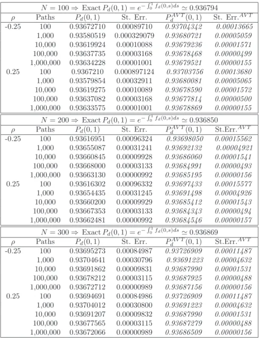
The numerical results for the simulations of time zero bond prices with one year ma-turity are displayed in Table 1. Here and in all the Tables we use the Antithetic Variable technique in order to improve numerical accuracy and reduce computational effort. In Table 1 the third and fourth columns refer to the results obtained with the plain Monte Carlo Algorithm, while the last two columns are obtained with the Antithetic Variable technique. For each discretisation (N = 100, 200,300) the exact defaultable bond prices are calculated and can be compared in Table 1 to the simulated bond prices obtained by varying the number of paths and the correlation coefficient. This comparison gives us one test of the efficiency of the algorithm and verifies the accuracy of the numerical method. In Table 1 we illustrate the impact on the standard error of variations of N and Π. In particular, in the case of one million paths, the standard error becomes significant at only the fifth decimal place. We use both negative and positive correlation values, even though the negative correlation is the more consistent with the observed market situation.
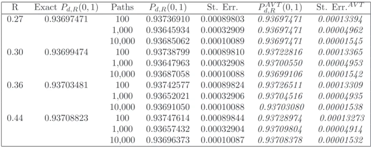
In the case of positive recovery rate, the value Pk
d,R(0, N∆t)is approximated by Pk d,R(0, T) =R e− PN−1 j=0 rk(j∆t)∆t+ (1−R)e− PN−1 j=0 [rk(j∆t)+λk(j∆t)]∆t, (38)
and again the Monte Carlo bond price may be computed. Table 2 shows the simulated initial price of a bond maturing in one year usingΠ = 100/1,000/10,000respectively, using
recovery rates observed in the market (see Moody’s Investors Service (2007)) and N =
200. In this case we assume only negative correlation. Also in this case we can compare simulated results with the actual ones and independently of the recovery rate value, the method reaches an accuracy of almost four decimal figures after 10,000 simulated paths.
PAV T
d andSt. ERR.AV T represent respectively the evaluation using the Antithetic Variable
technique and its standard error. The reduction in the standard errors demonstrates the effectiveness of this technique.
We now consider the general case in which we wish to evaluate at timet0,0≤t0 ≤T ≤
T, a defaultable bond with maturityT and zero recovery rate. We simulate the evolution of the function f(t, τ), τ ≥ t, τ ∈ [0, T], with t varying in [0, t0]. For every t ∈ [0, t0] we obtain therefore an approximation to the curve f(t, τ), τ ≥ t. We simulate Q evolutions of the curve and for each k−thsimulated curve at time t0, we calculate the corresponding bond value
Pk
d(t0, T) = e−
RT
so that the price at t0, evaluated at 0, of a bond price with maturity T, that we denote
Pd(0, t0, T), is calculated according to
Pd(0, t0, T) = EPe[Pd(t0, T)|F0], which can be approximated by the Monte Carlo method as
PM C d (0, t0, T) = 1 Q Q X k=1 Pk d(t0, T)'EPe[Pd(t0, T)|F0].
For these calculations we simply use the Euler-Maruyama integral approximation
Z T t0 fk d(t0, s)ds= NX−1 i=n fk d(n∆t, i∆t)∆t.
The numerical results are shown in Table 3. We calculate the value of a zero coupon bond with 5-year maturity at timet = 2and of a zero coupon bond with 10-year maturity at time
t = 5. The effect of different combinations of (N,Π) on the standard error is shown and the best accuracy is obtained with N = 500, Π = 10,000. More accurate approximations are obtained in the sixth column by applying the AV technique.
Turning now to the credit default swap, we assume at time tthe purchase of a CDS on a defaultable zero coupon bond with maturity T and recovery rate R. The contract gives protection against a default event occurring at time τ over the single interval [Tk−1, Tk],
where we recall thatTk=k∆t,Tk−1 = (k−1)∆t and T =N∆t.
Using the Monte Carlo simulation approach above we obtain the approximate fair rate
S(0) at time zero as
SMC(0) = (1−R)PdM C(0,(k−1)∆t)−PdM C(0, k∆t) (k∆t−(k−1)∆t)PM C
d (0, k∆t)
. (39)
In Table 4 we display numerical results for a credit default swap contract on a risky zero coupon bond with recovery rate 0.30 and maturity 3 years, denoted Pd,0.3(0,3) and we takeN = 300. The protection buyer pays a fee S(0)in exchange for protection against a default occurring at timeτ over the interval[0,1]. In the first row of the table, the exact CDS rate, calculated using formula (30), is displayed. The accuracy of the approximation improves by increasing the number of paths. The standard error is significant at the fourth decimal place. The fourth and fifth columns display the results obtained with the variance reduction technique.
Finally, we consider the credit default swap option. To price this we need to evaluate at time zero a call option with maturity Ts, 0 < Ts < T, issued on a CDS. Under the
terms of the CDS, the protection buyer pays a fixed fee K in exchange for a contingent payment(1−R)upon a credit event occurring over the period [Ts, T]. The CDSO value is
equal to the expected value of the discounted payoff at maturity date with respect to the risk-neutral measure Pe, namely (see equation (33))
CDSO(0, Ts, T) = 1{τ >0}EPe £ Pd(0, Ts) © (T −Ts)Pd(Ts, T) ª (S(Ts)−K)+|H0 ¤ . (40)
In the numerical scheme the option maturity times are Ts =n∆t and T = N∆t and the
Monte Carlo price is given as
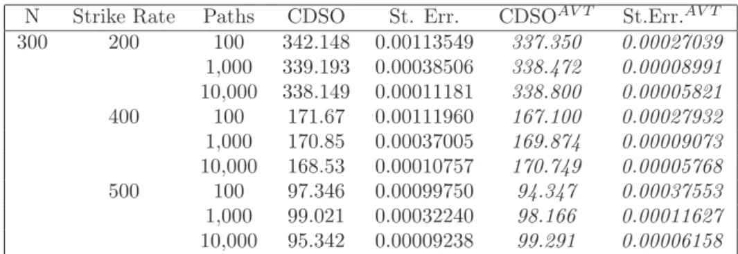
CDSOM C(0, n∆t, N∆t) = Q1 Q X k=1 CSDOk(0, n∆t, N∆t), (41) where CDSOk(0, n∆t, N∆t) = PkM C d (0, n∆t) © (N∆t−n∆t)PkM C d (n∆t, N∆t) ª (Sk(n∆t)−K)+. (42) In Table 5 we present the numerical results for the CDSO calculations. At time zero we price a call option with maturity date Ts = 2 issued on a CDS. The CDS has a zero
coupon bond Pd,0.30(0,3) as its underlying and the default protection period is [2,3]. We
implement the model using different strike prices and N = 300. The simulated prices
reflect the actual market behaviour as they decrease when the strike rate increases. On the contrary, the results shown in Table 6 are related to prices of the call option according to different numbers of paths, when the strike rate is equal to 200 bp. In both tables Monte Carlo simulations with the number of paths equal to 1,000, already gives a CDSO value with three decimal accuracy. The last two columns in both tables show the AV technique results.
We can observe that the AV method’s standard error always turns out to be one quarter of the standard error obtained by the standard Monte Carlo method. The accuracy of the prices increases by one decimal place with the application of the AV technique. Results displayed in the Tables 1-6 show how the accuracy of the numerical computations increases with N and with the number of simulations Π. Besides, by observing the results we verify that the AV technique is efficient because it fulfills the condition of effectiveness, namely
2V ar(CDSOAV T)≤V ar(CDSO). (43) In our final analysis we seek to assess the efficiency of the algorithm in terms of runtimes. We compute the root mean-square deviation (RMSD) of the one year maturity zero coupon bond price, P(0, N∆t), from the “true” value, PT r(0, N∆t), using AV technique Monte
Carlo bond prices with 100, 1,000, 10,000 and 100,000 paths, with values of N of 100, 200 and 300 and correlation ±0.25. The “true” price is estimated using 1,000,000 paths
according with N =100, 200 and 300. Then, for eachN, we compute the RMSDs:
RMSDΠ= v u u t1 Π Π X i=1 (Pi(0, N∆t)−PT r(0, N∆t))2
with Π = 100; 1,000; 10,000; 100,000. In Table 7 we provide the RMSD values and the corresponding runtimes for different N and Π in the case of positive and negative cor-relations. We find that increasing the number of paths, the pricing accuracy improves, confirming the previous considerations made about the AV technique results (Table 1). Clearly, both in the case of correlation coefficient equal to −0.25 and 0.25, the algorithm runs faster when N = 100 than in the other cases. In particular, for each Π, the runtime
triples by increasing the discretisation from 100 to 200 and it doubles when N goes from 200 to 300. In contrast, for a given Π, the accuracy basically remains unchanged when
N = 100,200 and 300. For each N, by increasing the number of paths from 100 to 1,000 the accuracy improves by one decimal place, while it remains basically unchanged moving from 1,000 to 10,000 paths. The best accuracy trade-off is obtained with 100,000 paths: for all discretisations the accuracy improves by two decimal places with respect to the one obtained with Π = 100. This allows us to assert that the best efficiency trade-off of the algorithm is obtained withN = 100, because runtimes are the lowest. With regard to the number of simulated paths, the choice will depend on the accuracy required. Data shown in Table 7 are plotted in Figures 1-6. On the horizontal axis we measure the runtimes (sec-onds) on a logarithm scale in order to better highlight the computational time differences among the computed values. On the vertical axis the RMSDs are reported. The Figures are a more intuitive representation of the Table 7 data and they allow the reader to more readily appreciate the conclusions drawn above.
5
Conclusions
We have developed an HJM model for the defaultable interest rate term structure when the forward rate volatility functions depend on time to maturity, on the instantaneous defaultable spot rate and on the entire forward curve. The Cox process describes the default event and its intensity denotes the credit spread.
The described volatility functions are path dependent and therefore difficult to han-dle both analytically and numerically. Using a simple numerical scheme, based on the Euler-Maruyama discretisation of stochastic integrals, we develop an algorithm to simu-late the evolution of the entire defaultable curve over the time horizon in an efficient way. A more detailed discussion of the numerical scheme and further numerical results of its implementation are provided by Fanelli (2007).
The expected bond value conditional on the realization of the Cox process intensity is computed by using an inhomogeneous Poisson process. In this way, the explicit reference to the default event is eliminated and is defined as a function of the default process intensity. We use the Monte Carlo method to calculate the defaultable bond price both in the case of zero recovery rate and positive recovery rate. The numerical results indicate the algorithm’s efficiency for evaluating corporate bonds and credit derivatives. The developed pricing algorithm also allows the evaluation of forward risky bond prices. Furthermore, we develop a numerical algorithm for CDS and CDS option pricing. The Antithetic Variable technique improves the accuracy of the simulated prices by reducing the standard error.
The numerical analysis is completed with the study of the trade off between runtimes and accuracy, suggesting the suitable combinations of number of paths/level of discretisa-tion, in order to reach the accuracy required in the price evaluations. The analysis indicates how the algorithm can be successfully utilized by credit risk practitioners in order to price credit risk products with satisfactory accuracy levels and reasonable runtimes.
As the number of credit derivatives grows continuously, new approaches for their eval-uation are required. Consequently, future research will need to develop new algorithms for the evaluations of other more exotic type credit derivatives, such as basket products.
HJM framework is used to model the term structure evolution of electricity forward/futures prices and the contracts of interest have various types of exotic features, such as swing options.
A
Tables of Numerical Results
Table 1: I-Time zero ZCB Price N = 100⇒ ExactPd(0,1) =e−
R1
0fd(0,s)ds'0.936794
ρ Paths Pd(0,1) St. Err. PdAV T(0,1) St. Err.AV T
-0.25 100 0.93672710 0.00089710 0.93704342 0.00013665 1,000 0.93580519 0.000329079 0.93680721 0.00005059 10,000 0.93619924 0.00010088 0.93679236 0.00001571 100,000 0.93637735 0.00003168 0.93678468 0.00000499 1,000,000 0.93634228 0.00001001 0.93679521 0.00000155 0.25 100 0.9367210 0.000897124 0.93703756 0.00013680 1,000 0.93579854 0.00032911 0.93680081 0.00005065 10,000 0.93619275 0.00010089 0.93678590 0.00001572 100,000 0.93637082 0.00003168 0.93677814 0.00000500 1,000,000 0.93633575 0.00001001 0.93678869 0.00000155 N = 200⇒ ExactPd(0,1) =e− R1 0fd(0,s)ds'0.936850
ρ Paths Pd(0,1) St. Err. PdAV T(0,1) St.Err.AV T
-0.25 100 0.93616951 0.00096324 0.93698050 0.00015562 1,000 0.93655087 0.00031241 0.93692132 0.00004921 10,000 0.93660845 0.00009928 0.93686060 0.00001541 100,000 0.93668000 0.00003133 0.93684991 0.00000493 1,000,000 0.93663130 0.00000992 0.93685195 0.00000156 0.25 100 0.93616302 0.00096332 0.93697433 0.00015577 1,000 0.93654435 0.00031245 0.93691498 0.00004926 10,000 0.93660200 0.00009929 0.93685412 0.00001543 100,000 0.93667353 0.00003133 0.93684343 0.00000494 1,000,000 0.93662481 0.00000992 0.93684546 0.00000157 N = 300⇒ ExactPd(0,1) =e− R1 0fd(0,s)ds'0.936869
ρ Paths Pd(0,1) St. Err. PdAV T(0,1) St.Err.AV T
-0.25 100 0.93695273 0.00084987 0.93726909 0.00011487 1,000 0.93704641 0.00030796 0.93691223 0.00004632 10,000 0.93691862 0.00009831 0.93687990 0.00001531 100,000 0.93678212 0.00003115 0.93687925 0.00000488 1,000,000 0.93672712 0.00000989 0.93687156 0.00000156 0.25 100 0.93694691 0.00084986 0.93726909 0.00011487 1,000 0.93704012 0.00030800 0.93691223 0.00004632 10,000 0.93691207 0.00009832 0.93687990 0.00001531 100,000 0.93677565 0.00003115 0.93687279 0.00000488 1,000,000 0.93672066 0.00000989 0.93686509 0.00000156
Table 2: Time zero ZCB Prices in the case of positive recovery rate (R)
R ExactPd,R(0,1) Paths Pd,R(0,1) St. Err. Pd,RAV T(0,1) St. Err.AV T
0.27 0.93697471 100 0.93736910 0.00089803 0.93697471 0.00013394 1,000 0.93645934 0.00032909 0.93697471 0.00004962 10,000 0.93685062 0.00010089 0.93697471 0.00001545 0.30 0.93699474 100 0.93738799 0.00089810 0.93722816 0.00013365 1,000 0.93647963 0.00032908 0.93700550 0.00004953 10,000 0.93687058 0.00010088 0.93699106 0.00001542 0.36 0.93703481 100 0.93742577 0.00089824 0.93726511 0.00013309 1,000 0.93652021 0.00032906 0.93704516 0.00004935 10,000 0.93691050 0.00010088 0.93703080 0.00001538 0.44 0.93708823 100 0.93747614 0.00089844 0.93728974 0.00013273 1,000 0.93657432 0.00032904 0.93709804 0.00004914 10,000 0.93696373 0.00010087 0.93708378 0.00001532
Table 3: Forward ZCB Prices
ρ N Paths Pd(0,2,5) St.Err. PdAV T(0,2,5) St.Err.AV T
-0.25 500 100 0.77723533 0.00384184 0.77869190 0.00107819 1,000 0.77870174 0.00131634 0.77929703 0.00039613 10,000 0.77930372 0.00041341 0.77931346 0.00010909 0.25 100 0.777138976 0.00383949 0.77859926 0.00107728 1,000 0.77859938 0.00131551 0.77919335 0.00039684 10,000 0.77919522 0.00041326 0.77923799 0.00010945
ρ N Paths Pd(0,5,10) St.Err. Pd(0,5,10)AV T St.Err.AV T
-0.25 1,000 100 0.64604114 0.005267 0.64792752 0.00359192
1,000 0.65095188 0.00183757 n.a. n.a. 0.25 100 0.64589044 0.00525009 0.64774897 0.00360483
1,000 0.65072434 0.00183321 n.a. n.a.
n.a. =not available
Table 4: Time zero Credit Default Swaps on a risky zero coupond bond with R= 0.3and maturity of 3 years
Exact CDS=470.499 bp
Paths CDS Rate St.Err. CDSAV T Rate St.ErrAV T
100 468.847 0.00073091 469.509 0.00026824
1,000 469.089 0.00027412 470.219 0.00010172
10,000 469.498 0.00008365 n.a. n.a.
Table 5: I-Time zero CDSO Prices
N Strike Rate Paths CDSO St. Err. CDSOAV T St.Err.AV T
300 200 100 342.148 0.00113549 337.350 0.00027039 1,000 339.193 0.00038506 338.472 0.00008991 10,000 338.149 0.00011181 338.800 0.00005821 400 100 171.67 0.00111960 167.100 0.00027932 1,000 170.85 0.00037005 169.874 0.00009073 10,000 168.53 0.00010757 170.749 0.00005768 500 100 97.346 0.00099750 94.347 0.00037553 1,000 99.021 0.00032240 98.166 0.00011627 10,000 95.342 0.00009238 99.291 0.00006158
Table 6: II-Time zero CDSO Prices
Strike rate N Paths CDSO St. Err. CDSOAV T St.Err.AV T
200 300 100 342.148 0.00113549 337.350 0.00027039 1,000 339.193 0.00038506 338.472 0.00008991 10,000 338.149 0.00011181 338.800 0.00005821 600 100 350.523 0.00134806 341.788 0.00032076 1,000 341.322 0.00038406 341.778 0.00009147 10,000 338.704 0.00011164 341.481 0.00003511
Table 7: Accuracy vs Runtimes ρ=-0.25
N=100 N=200 N=300
Paths RMSD Runtime Paths RMSD Runtime Paths RMSD Runtime 100 1.39×10−04 0.953 100 1.56×10−04 3.406 100 1.22×10−04 6.953 1,000 5.06×10−05 9.531 1,000 4.93×10−05 31.781 1,000 4.63×10−05 69.406 10,000 1.57×10−05 92.015 10,000 1.54×10−05 316.031 10,000 1.53×10−05 693.938 100,000 4.99×10−06 842.422 100,000 4.98×10−06 3,813.730 100,000 4.88×10−06 6,998.060 ρ=0.25 N=100 N=200 N=300
Paths RMSD Runtime Paths RMSD Runtime Paths RMSD Runtime 100 1.39×10−04 0.875 100 1.56×10−04 3.171 100 1.22×10−04 69.531
1,000 5.07×10−05 8.734 1,000 4.93×10−05 31.484 1,000 4.63×10−05 69.734
10,000 1.57×10−05 88.078 10,000 1.54×10−05 321.625 10,000 1.53×10−05 691.734
Accuracy vs Runtimes of Simulated ZCB Price 0 2 4 6 8 10 12 14 16 0.95 9.53 92.01 842.42 Time (sec) R M S D ( x 1 0 ^ -5 ) 100 paths 1,000 paths 100,000 paths 10,000 paths Figure 1: N=100,ρ=−0.25 0 2 4 6 8 10 12 14 16 0.87 8.73 88.07 963.85 Time (sec) R M S D ( x 1 0 ^ -5 ) 100 paths 1,000 paths 10,000 paths 100,000 paths Figure 2: N=100, ρ=0.25 0 2 4 6 8 10 12 14 16 18 3.40 31.78 316.03 3,813.73 Time (sec) R M S D ( x 1 0 ^ -5 ) 1,000 paths 100 paths 10,000 paths 100,000 paths Figure 3: N=200,ρ=−0.25 0 2 4 6 8 10 12 14 16 18 3.17 31.48 321.62 3,421.39 Time (sec) R M S D ( x 1 0 ^ -5 ) 100 paths 1,000 paths 10,000 paths 100,000 paths Figure 4: N=200, ρ=0.25 0 2 4 6 8 10 12 14 6.95 69.40 693.93 6,998.06 Time (sec) R M S D ( x 1 0 ^ -5 ) 100 paths 1,000 paths 10,000 paths 100,000 paths Figure 5: N=300,ρ=−0.25 0 2 4 6 8 10 12 14 6.95 69.73 691.73 6,922.59 Time (sec) R M S D ( x 1 0 ^ -5 ) 100 paths 1,000 paths 10,000 paths 100,000 paths Figure 6: N=300, ρ=0.25
B
The HJM model for the defaultable term structure
From equation (12) and the assumed dynamics of f(t, T) and λs(t, T), the HJM forward
defaultable term structure dynamics may be expressed in the form
dfd(t, T) =α(t, T,·)dt+αλ(t, T,·)dt+σ(t, T,·)dW(t) +σλ(t, T,·)dWλ(t). (44)
Integrating both sides, we obtain the instantaneous defaultable forward rate expressed in the integral form
fd(t, T) =f(0, T) +λs(0, T) + Rt 0 α(v, T,·)dv+ Rt 0 αλ(v, T,·)dv +R0tσ(v, T,·)dW(v) +R0tσλ(v, T,·)dWλ(v), (45) where:
- f(0, T) and λs(0, T) are, respectively, the initial forward risk-free rate curve and the
initial forward spread curve, observable at time t = 0;
- α(t, T,·) andαλ(t, T,·)are the instantaneous drift functions of the risk-free forward rate
and credit spread, where the third argument indicates the possible dependence on other path dependent variables, such as the spot rate, the forward rate itself or the credit spread;
- σ(t, T,·)and σλ(t, T,·)are the instantaneous volatility functions of the risk-free forward
rate and credit spread, where, as above, the third argument indicates the aforemen-tioned possible dependence on other path dependent variables, such as the spot rate, the forward rate itself or the credit spread;
- W(t)and Wλ(t) are Wiener processes with respect to the objective probability measure
P.
In the following, we denote the price of a defaultable ZCB with zero recovery rate as
Pd(t, T). Therefore, in the case of no default, we have:
Pd(t, T) = e− RT
t fd(t,s)ds =e− RT
t (f(t,s)+λs(t,s))ds. (46)
By the use of Fubini’s Theorem for the stochastic integral and application of Ito’s lemma, the defaultable bond price is found to satisfy the stochastic differential equation
dPd(t, T) = [r(t) +λ(t) +b(t, T) +bλ(t) +ρa(t, T)aλ(t, T)]Pd(t, T)dt +a(t, T)Pd(t, T)dW(t) +aλ(t, T)Pd(t, T)dWλ(t), (47) where ( a(v, t) :=−Rvtσ(v, s)ds, aλ(v, t) :=− Rt v σλ(v, s)ds, (48)
and ( b(v, t) = −Rvtα(v, s)ds+1 2a(v, t)2, bλ(v, t) =− Rt v αλ(v, s)ds+12aλ(v, t)2. (49) Equation (47) can be also written in return form as
dPd(t, T)
Pd(t, T)
= [r(t) +λ(t) +b(t, T) +bλ(t) +ρa(t, T)aλ(t, T)]dt
+a(t, T)dW(t) +aλ(t, T)dWλ(t). (50)
In order to obtain the no arbitrage condition, we start from (50) and apply the Schön-bucher (1998) approach and the Björk (2004) methodology. That is we apply the economic principle that the expected excess return on the defaultable bond is equal to the risk pre-mium. Thus keeping in mind that a(t, T) and aλ(t, T) are respectively “the amounts of
risk” associated with the Wiener increments dW(t) and dWλ(t) we write [r(t) +b(t, T) +bλ(t, T) +ρa(t, T)aλ(t, T)]−r(t) =
φ(t)a(t, T) +φλ(t)aλ(t, T), (51)
whereφis the market price of interest rate (W(t)) risk andφλis the price of spread (Wλ(t))
risk. Equation (51) is the “martingale measure equation”. It allows the transition from the actual risky world under the objective P measure to the risk neutral world under the measure Pe. On the left-hand side we have the excess rate of return for the defaultable bond over the risk-free rate, and on the right-hand side we have the linear combination of the volatilities and market prices of risk that yield the instantaneous risk premium. Some simple rearrangements express (51) in the more convenient form
b(t, T)−φ(t)a(t, T) +bλ(t, T)−φλ(t)aλ(t, T) +ρa(t, T)aλ(t, T) = 0. (52)
By substituting (48) and (49) into (52) we obtain − Z T t α(t, s)ds+1 2 µZ T t σ(t, s)ds ¶2 − Z T t αλ(t, s)ds +1 2 µZ T t σλ(t, s)ds ¶2 +ρ Z T t σ(t, s)ds Z T t σλ(t, s)ds +φ(t) Z T t σ(t, s)ds+φλ(t) Z T t σλ(t, s)ds= 0. (53)
By differentiating with respect to T, the above expression can be rewritten in the form −α(t, T) +σ(t, T) Z T t σ(t, s)ds−αλ(t, T) +σλ(t, T) Z T t σλ(t, s)ds+ρσ(t, T) Z T t σλ(t, s)ds +ρσλ(t, T) Z T t σ(t, s)ds−φ(t)σ(t, T)−φλ(t)σλ(t, T) = 0. (54)
From (54) we can obtain the HJM forward rate drift restriction for defaultable processes, namely αd(t, T) =α(t, T) +αλ(t, T) =σ(t, T) Z T t σ(t, s)ds+σλ(t, T) Z T t σλ(t, s)ds +ρ · σ(t, T) Z T t σλ(t, s)ds+σλ(t, T) Z T t σ(t, s)ds ¸ −φ(t)σ(t, T)−φλ(t)σλ(t, T). (55)
We define two new processes
f W(t) =W(t) + Z t 0 (−φ(s))ds, (56) and f Wλ(t) =Wλ(t) + Z t 0 (−φλ(s))ds, (57) so that dfW(t) =dW(t)−φ(t)dt, (58) and dfWλ(t) =dWλ(t)−φλ(t)dt. (59)
For later calculations we note that the last two equations imply that
dW(t) =dWf(t) +φ(t)dt, (60) and
dWλ(t) =dWfλ(t) +φλ(t)dt. (61)
By an application of Girsanov’s Theorem fW(t)and Wfλ(t) will be Wiener processes under e
P. By substituting (55), (60) and (61) into (44) we obtain
dfd(t, T) = · σ(t, T) Z T t σ(t, s)ds+σλ(t, T) Z T t σλ(t, s)ds +ρσ(t, T) Z T t σλ(t, s)ds+ρσλ(t, T) Z T t σ(t, s)ds ¸ dt +σ(t, T)dfW(t) +σλ(t, T)dWfλ(t). (62)
By integrating, we obtain the instantaneous defaultable forward rate dynamics in stochastic integral equation form, namely
fd(t, T) =f(0, T) +λs(0, T) + Z t 0 · σ(v, T) Z T v σ(v, s)ds+σλ(v, T) Z T v σλ(v, s)ds ¸ dv + Z t 0 ρ · σ(v, T) Z T v σλ(v, s)ds+σλ(v, T) Z T v σ(v, s)ds ¸ dv + Z t 0 h σ(v, T)dWf(v) +σλ(v, T)dWfλ(v) i . (63)