Saïd Business School
Research Papers
Saïd Business School RP 2017-18
The Saïd Business School’s working paper series aims to provide early access to high-quality and rigorous academic research. Oxford Saïd’s working papers reflect a commitment to excellence, and an interdisciplinary scope that is appropriate to a business school embedded in one of the world’s major research universities.
The Lender of Last Resort in a General Equilibrium
Framework
Akshay Kotak
Saïd Business School, University of Oxford
Han N. Ozsoylev
Saïd Business School, University of Oxford
Dimitrios Tsomocos
Saïd Business School, University of Oxford
October 2017
The Lender of Last Resort in a General Equilibrium Framework
∗Akshay Kotak†1, Han N. Ozsoylev‡2, and Dimitrios Tsomocos§3 1Saïd Business School and Green Templeton College, University of Oxford
2Koç University, and Saïd Business School, University of Oxford 3Saïd Business School and St. Edmund Hall, University of Oxford
October 15, 2017
Abstract
This paper models the role of the lender of last resort (LoLR) in a general equilibrium framework. We allow for heterogeneous agents and a risk-averse banking sector, and incorporate the frictions of endogenous default, liquidity, and money. Adverse supply shocks in monetary endowments trig-ger default, leading to deterioration in the value of bank assets, and subsequent bank illiquidity in some states of the world. LoLR intervention is then assessed with regards to its economy-wide effect on welfare, bank profitability, and the level of default. The results provide a rationalisation for constructive ambiguity and the ‘too big to fail’ problem.
JEL Classification Numbers: E58, G21, G28
Keywords: Lender of last resort, default, bank bailouts, constructive ambiguity
∗
Acknowledgments: We would like to thank Kwangwon Ahn, Charles Goodhart, Li Lin, Thomas Noe, Udara Peiris, Oren Sussman, Alexandros Vardoulakis and Geoffrey Wood for their invaluable advice and comments. Kotak would also like to thank the Saïd Foundation for financial support. All errors herein are ours.
† [email protected] ‡ [email protected] § [email protected] 1
1
Introduction
The concept of the lender of last resort (LoLR) traces its origins to the works of Henry Thorn-ton (1802) and Walter Bagehot (1873) who outlined measures that the Bank of England need undertake to ensure the sound functioning of the British banking system in times of crisis. As outlined in Humphrey (1989), this classical paradigm of the LoLR as envisioned by Thornton and Bagehot, stressed “protecting the aggregate money stock, not individual institutions; let-ting insolvent institutions fail; accommodalet-ting sound institutions only; charging penalty rates; requiring good collateral; and preannouncing these conditions well in advance of any crisis so that the markets know exactly what to expect.”1
Bordo (1990) lists four major schools of thought regarding the role of the LoLR: The first is the classical paradigm of Thornton (1802) and Bagehot (1873) wherein the LoLR has a clearly articulated policy of lending to any bank that is illiquid but solvent, at a penalty rate,2 and against sound collateral (valued at pre-crisis prices).3 The second is the doctrine prompted by Goodfriend and King (1988) who argue that the LoLR need only intervene to provide aggregate liquidity to the banking sector by way of open market operations. They assert that LoLR assistance to individual institutions is similar to the private provision of line-of-credit services in that it requires costly monitoring. They, therefore, deem it redundant given the development of the interbank market and assert that it encourages excessive risk taking. The third school of thought, based on the work of Goodhart (1987, 1988, 1999), argues that the LoLR cannot disentangle temporary liquidity shocks from permanent solvency shocks, and therefore advocates basing assistance on several factors, including the wider implications of the choice between assistance and refusal, as well as the assessed conditions of the banks in difficulties.4 Finally, the fourth school of thought proposes free banking with no regulatory intrusion.5 Bordo (1990) surveys the literature on free banking and concludes, based on historical evidence, that there is normally a need for a monetary authority to act as the lender of last resort. This would be especially true in the face of a major aggregate shock that produces a widespread demand for
1
The vast body of literature on the topic that has since accumulated has been extensively surveyed by Freixas et al. (2000).
2
As noted in Goodhart (1999), Bagehot did not explicitly use the term ‘penalty’ rate. Goodhart asserts that by use of the phrase ‘high rate of interest’, Bagehot meant a rate above the market rate prior to the crisis, but not necessarily higher than that prevailing at the time of LoLR action.
3Rochet and Vives (2004) present a modern reformulation of the classical Bagehotian doctrine in a model
with a developed interbank market. Unlike standard models of coordination failure, their model does not rely on the multiplicity of equilibria but has a unique Bayesian equilibrium in which an illiquid but solvent bank is, with positive probability, unable to find liquidity assistance in the interbank market. This prompts the need for LoLR intervention coupled with other policy measures.
4This view is contended by Bordo (1990) who claims that assistance to insolvent banks was the exception
rather than the rule until the 1970s, and that “liberal assistance to insolvent banks, combined with deposit insurance which is not priced according to risk, encourages excessive risk-taking, creating the conditions for even greater assistance to insolvent banks in the future.”
5Goodhart (1988, 1995) states that Bagehot (1873) supported the theoretical idea of a free banking regime
with no government intrusion, but felt that it would be too unrealistic to implement and thus sought to reform the Bank of England as the next best option.
high-powered money, a problem that a laissez faire, unregulated system of commercial banks cannot adequately tackle.
While there is still much debate about the goals and objectives of a lender of last resort, it seems to have been satisfactorily established that they should exist, and this issue has come to the fore again in light of the recent financial crisis.6 There has been dissent, particularly because of the issue of moral hazard, dating all the way back to the nascent days of central banking, as evinced in the writings of François-Nicolas Mollien (1845) and Herbert Spencer (1878). However, as Goodhart (1987) and Kindleberger and Aliber (2011) have noted, with the evolution of the banking system and the looming spectre of contagion, there is a fairly convincing case for intervention. Bordo (1986, 1990) provides extensive historical evidence and asserts that a public body, acting as LoLR serves to abate financial crises. Goodhart and Schoenmaker (1995) study a sample of 104 bank crises across 24 countries between the 1980s and early 1990s. Of these, 73 ended up in bailouts, and in 20 of the remaining 31 cases (which ended in liquidation), deposit insurance payments were made. Rosas (2006) studies 46 cases of bank bailouts and develops a model of government policy response based on several key institutional parameters. He finds that good Bagehotian LoLR responses tend to occur in relatively closed economies, under a democratic regime, that suffer a macroeconomic shock. He also stresses the importance of sound institutions to complement such policy responses.
The aim of this study is to address the hitherto unattempted task of modelling the lender of last resort function in a general equilibrium framework. A general equilibrium approach with its tenets of “agent optimization, market clearing (i.e., perfect competition with flexible prices), and rational expectations” (Geanakoplos and Tsomocos, 2002) is desirable to study the interaction between the real and banking sectors. Additionally, the modelling approach chosen here allows for heterogeneous agents, endogenous default, liquidity, and money – all critical elements in studying a model of financial crises in the tradition of Fisher (1933), Minsky (1977), Allen and Gale (1999, 2000), and Kindleberger and Aliber (2011).
To this end, we design a two-period monetary general equilibrium model with heterogeneous households and a risk averse banking sector, represented by a single bank,7 and incorporate the frictions of default and money. The model is based on the work of Goodhart et al. (2010), which itself builds upon earlier works by Goodhart et al. (2004, 2005, 2006a,b), and Tsomocos (2003). At the outset, we model a strategic game between the commercial bank and the LoLR wherein each is unaware of the other’s strategy but their payoff functions are common knowledge. The bank chooses between an (exogenous) investment profile that has high tail risk, and one that has low tail risk, and this choice affects its endowments in different states in the future.
6
See Barrell and Davis (2008); Bordo (2008).
7We concede that our current one-bank model underestimates the contagion effect of default, and therefore
underestimates the importance of LoLR action in stemming contagion in a system with heterogeneous banks. Additionally, since our model has only two periods, the charter value of the bank in the second period goes to zero. This overstates the moral hazard implications of LoLR assistance, as in an infinite horizon model the
If it chooses a profile with high tail risk, it ends up with relatively higher endowment in good states of nature but ends being illiquid in bad states of nature. A low tail risk profile on the other hand, ensures that the bank remains liquid in all future states of nature. The central bank acting as the LoLR, unaware of the exact nature of the bank’s balance sheet, may choose
ex ante to adopt a doveish stance and bail the distressed bank out or be hawkish and liquidate the bank.8 The strategic choices of the commercial bank and the LoLR determine the set of decision variables and the budget sets of all agents, and the economy subsequently attains the corresponding general equilibrium.
The economy modelled is one of exchange without production. Households maximize ex-pected utility from the consumption of a single good, across both time periods and across all states of nature. The commercial bank issues short term loans to provide liquidity in the mar-ket, since households are subject to cash-in-advance constraints. It also issues inter-period loans for agents to borrow against expected future earnings. The bank itself borrows from depositors, and from the central bank in the form of repo loans, pledging its future monetary endowment as collateral. This endowment may be thought of as other (exogenous) assets of the bank. Based on the bank’s ex ante choice of risk profile, and the state of nature realised, it may end up in a state where its monetary endowment has lower value than its loan obligations, forcing it to default on its repo loan – and depending on the LoLR’s stance, it may or may not be bailed out. This has implications for the default decisions of households, and affects the aggregate level of default in the economy. Default between the agents and the commercial bank is modelled as continuous default à la Shubik and Wilson (1977), that is, agents can partially (or fully) default on their debt obligations to the bank if they choose to do so.
It is also worth noting how the LoLR’s objective function is set up in our model. Current literature highlights the preservation of financial stability as one of the key roles of modern central banks (Ortiz, 2009; Goodhart, 2011). We aimed to formalise an objective function for the lender of last resort in keeping with this role. Following Goodhart et al. (2004) and Tsomocos (2003), we therefore set up an objective function for the LoLR that is increasing in banking sector profitability and decreasing in the aggregate level of default in the economy.
We calibrate the model described above to study the equilibrium strategies employed by the two players, namely, the bank and the LoLR. In our calibrated model, we find that the unique Nash equilibrium of the game is one of mixed strategies with the LoLR committing ex ante
to a strategy of bailing out the bank in some cases, and not in other cases.9 We consider this mixed-strategy Nash equilibrium to be a rationalisation of the policy ofconstructive ambiguity. In practice, constructive ambiguity has often been used to reduce moral hazard: Introducing
8
Another interesting setup would be to study the game as a sequential one with the LoLR deciding on a tough/soft policy stance and the commercial bank responding with a safe/risky investment profile. One would expect to find the time inconsistency problem with the LoLR not being credibly able to commit to a tough policy stanceex ante, analogous to that studied by Kydland and Prescott (1977).
9
Our aim here is to study what the optimalex antestance of the LoLR should be towards bailing out distressed banks in this framework. The issue of dynamic inconsistency of LoLR policy is beyond the scope of this study.
uncertainty about the availability of LoLR support can force banks to behave more prudently since they would no longer be certain of receiving assistance.
Our calibrations also reveal behaviour akin to the ‘too big to fail’ problem: We study com-parative statics of the relative importance of aggregate default in the LoLR’s objective function. We find that, the higher this relative importance is, the LoLR is more likely to bail out the bank in equilibrium. As a result, the bank is also more likely to choose an investment profile with high tail risk. In other words, the greater the perceived spillover effects of the bank’s failure are, the more the bank can hold the LoLR to ransom and pile on risk.
Obtaining a micro-founded rationalisation of constructive ambiguity and the ‘too big to fail’ problem, in a general equilibrium framework with both real and banking sectors, is a novel contribution of this paper. Most of the related literature focuses solely on the interaction be-tween commercial banks and the LoLR while investigating these issues. For instance, Freixas (1999), Freixas et al. (2000) and Freixas et al. (2004) study constructive ambiguity, and more generally, the role of the lender of last resort in such partial equilibrium settings.10 The theo-retical justification of constructive ambiguity in these papers is based on the classic arguments for discretion and the need for flexibility to allow a central bank to retain credibility.11 The ‘too big to fail’ problem has also been theoretically rationalised in the related literature on LoLR, e.g., by Goodhart and Huang (2005). They develop a partial equilibrium macro-level model of the LoLR. Their main claim is that financial contagion caused by the failure of a bank induces panic and uncertainty and leads to more volatile financial markets wherein predicting behaviour becomes more difficult. This makes it harder to correctly execute remedial macro-policy. In the static setup of Goodhart and Huang (2005), the LoLR weighs the cost of the provision of emergency liquidity assistance to an illiquid bank that may turn out to be insolvent, against the loss from getting macro-policy (in this case, the level of high-powered money which is con-trolled through open market operations) wrong in the face of the failure of the bank. This setup results in it being optimal for the central bank to provide LoLR support to banks larger than a threshold size, since larger banks would induce more uncertainty and hence bring about a
10Freixas (1999) asserts that LoLR intervention is essentially equivalent to extending the benefits of deposit
insurance to uninsured claim holders and is therefore distortionary. However, there are externalities generated by bank failures especially in light of the intricate network of interbank relationships, as noted in Allen and Gale (1999), and the LoLR needs to weigh the benefits of curbing a contagious systemic panic in the present against the cost of potential increases in risk taking in the future. Freixas et al. (2004) study optimal LoLR policy in the face of such moral hazard and find that LoLR intervention improves efficiency if the source of moral hazard is in the incentives for banks to screen loans. If instead, the source is in loan monitoring by banks, then the LoLR should not intervene and the interbank markets would discipline banks that engage in excessive risk taking. Freixas et al. (2000) note constructive ambiguity can be introduced in a variety of styles – uncertainty about whether assistance will be offered at all, about the timing of assistance, and about the conditions that come attached with the offer of assistance.
11
Enoch et al. (1997) claim that another justification for ambiguity is that optimal policy rules are a function of perfect and complete information – something that one almost never finds in banking. In the face of incomplete information, and given the short turnaround time available for critical LoLR intervention, even seemingly simple policy rules become hard to assess and implement. Affording regulators discretion in these cases helps minimize
larger expected loss due to incorrect macro-policy. This, of course, amplifies the moral hazard problem for big banks as they are deemed ‘too big to fail’ by the central bank.12
To the best of our knowledge, this paper is the first to study the lender of last of resort function in a general equilibrium framework. The payoff functions of both the LoLR and the bank are based on the competitive equilibrium values of the endogenous variables in the exchange economy. These endogenous variables include, among other things, interest rates, households’ default rates to the bank, and the bank’s re-payment rate on deposits. These variables of the exchange economy, in turn, depend on the strategic choices made by the LoLR and the bank, as the bank’s choice of investment risk profile affects households’ budget sets (through their borrowing constraints). Hence, the Nash equilibrium of the simultaneous game between the LoLR and the bank is linked to the competitive equilibrium of the exchange economy. We admit that our general equilibrium analysis is for now rudimentary in some aspects and we establish existence and (local) uniqueness of equilibrium only by calibration. Further research needs to be done on the general existence and uniqueness of equilibrium in this framework.
Section 2 below elaborates the strategic game, the structure of the economy modelled, the sequence of agent actions, and the market structure. Section 3 defines the equilibrium of the model and discusses its properties. A parametrised version of the model is presented in section 4. Section 5 details the comparative statics studied and section 6 concludes.
2
The model
2.1 Strategic game formulation
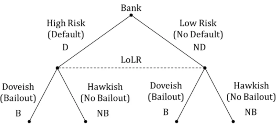
We model a strategic game between the commercial bank and the LoLR. The commercial bank borrows from the central bank (a proxy for the interbank market) through a repo loan which is collateralised. The bank’s monetary endowment is used to collateralise the loan and depending on itsex antechoice of risk profile, the bank may end up in a state where its monetary endowment has lower value than its loan obligations forcing it to default on the repo loan.13 The central bank acting as LoLR is unaware of the risk profile chosen the bank14, and has to determine its ex ante policy stance without knowledge of the risk profile chosen by the bank. We therefore have the following game tree:
12
Goodhart and Huang (2005) extend their analysis to a dynamic setup as well. In that setup, the probability of a future bank failure and the likelihood of an illiquid bank being insolvent are dependent on past LoLR actions and the optimal LoLR policy in this case is found to be non-monotonic in bank size, and time-varying.
13
We calibrate our model such that if the bank chooses a low risk profile, it is solvent in all future states of nature, whereas if it chooses a high risk profile, it defaults in bad states of nature.
14
In our calibration, we choose risk profiles that have the same expected value but differing riskiness (variance). This is in line with the asymmetry of information assumed in our game – the central bank may be able to assess the quality of collateral with regards to expected value but not in terms of riskiness.
Figure 1: Strategic game tree
The payoff function for the commercial bank is its expected lifetime utility as elaborated below in Section 2.7.3. We assume a plausible payoff function for the Central Bank (as the LoLR), in the spirit of Goodhart et al. (2004) and Tsomocos (2003). In these papers, financial fragility is characterised by an sharp decline in banking sector profitability coupled with a substantial increase in aggregate default. Financial fragility is detrimental since it precipitates welfare losses in the economy. The payoff of the Central Bank (as LoLR) is therefore chosen to be a simple, linear function of bank profitability (increasing) and the level of default in the economy (decreasing) less the costs of a bailout. These costs, denoted byC, include monetary costs of the bailout borne by taxpayers, and non-monetary costs such as a softening of banks’ budget constraints and a subsequent increase in moral hazard, and other political costs.
ΠCB =ξ1 X s∈S∗ θsπγs +ξ2 X s∈S∗ θs(1−νs)−C (1)
Formally, we have a strategic game Γ =
N,(Ai)i∈N,(Fi)i∈N
with:
A set of players: N ={Bank(γ), Central Bank - LoLR (CB)}
Action sets: Aγ ={Default (D), No Default (N D)} ACB ={Bailout (B), No Bailout (N B)}
Payoff functions: Fγ(a) = Πγ|(η,(σh)
h∈H)(a) ∀a∈Aγ×ACB
FCB(a) = ΠCB|(η,(σh)
h∈H)(a) ∀a∈Aγ×ACB
Note that the action Default (D) for the bank signifies choosing an investment profile with high tail risk (which is calibrated to ensure default in bad states of nature), it is not anex ante
choice to default in all future states of nature. Similarly, the action No Default (ND) signifies the bank choosing an investment profile with low tail risk, which ensures that it ends up being solvent in all states of nature.
endoge-choices (apart from its choice of exogenous risk profile) are continuous and competitively deter-mined in equilibrium and hence they are not strategic choices in the game. The LoLR’s payoff function is as defined in equation 1 above, and the bank’s payoff function is as defined in Section 2.7.3 below.
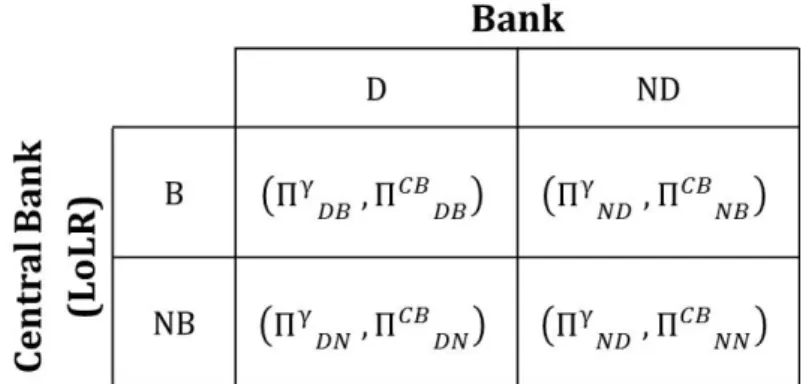
Figure 2: Payoff table for the strategic game
The risk profile chosen by the bank in the game is exogenous to the GE model but is linked to the quality of the collateral against which it borrows from the central bank and determines whether or not it will default in the bad state. The central bank is unaware of this strategic choice ex ante (and therefore doesn’t know ex ante whether the bank will default or not) – this is the information asymmetry at the heart of the simultaneous game and this is why even though the two players may not make their moves at the same time, de factothe game can be analysed as a simultaneous game the game since each player is unaware of the actions of the other. This asymmetry is resolved by the Nash Equilibrium of the simultaneous game.
2.2 The economy
The economy modelled is a two period, static world which includes two agent-households (α, β) and a representative commercial bank (γ). There are two time periods, and S possible states of nature in the second period. Statesoccurs with probabilityθs. There is a single, perishable
consumption good in this model. Households maximize the utility15of consumption of this good in each time period t ∈ T = {0,1}, and across each state of nature s ∈ S. Banks maximize their expected profits. The set of all states is denoted s∈S∗ ={0} ∪S. The set of all agents is denotedh∈H={α, β, γ}.
Household α is relatively wealthier at t = 0 while household β is relatively wealthier at
t = 1. The households therefore trade in order to smoothe consumption. Both households interact with the commercial bank γ. There is an exogenous cash endowment given to each household free of any obligation (ms ≥ 0, for s ∈ S∗). Endowments in goods and cash are
15
In our simulations, we use a constant relative risk aversion (CRRA) utility functionu(c) = c1−1−ρρ, to be able to consider wealth effects.
allowed to vary across states of nature.
Figure 3: Structure of the model
2.3 Money
Money is the stipulated means of exchange and store of value in this model. It is introduced through cash-in-advance constraints, implying that households can only purchase the consump-tion good by paying in cash. Money is fiat and has no consumpconsump-tion value but its value derives from the fact that it is essential to conduct trade in the goods market. The Central Bank controls the supply of money and injects it into the economy in both time periods. In the first period the commercial bank γ borrows from depositors and extends long term loans. It also uses its future monetary endowment as collateral to take on a repo loan from the Central Bank and provides short-term liquidity att= 0 to allow households to make purchases with cash. In the second period, the bank pays back depositors, the repo loan and issues short-term liquidity that is repaid at the end of the period when all the money exits the economy, since it has no consumption value.
2.4 Default
All loan contracts are defaultable in this model. Default, in our model, is endogenous and therefore a decision variable for agents. Short-term (intraperiod) loans, deposits and long-term (interperiod) loans are unsecured in our model. Default in these markets is therefore modelled as a continuous phenomenon as was first studied by Shubik and Wilson (1977) and was extended to a general equilibrium framework by Dubey et al. (2005). In this case, the repayment rate
face a non-pecuniary penalty which reduces utility by a constant rate ‘λ’ per monetary unit of account not repaid. The default penalties for the short-term loan, long-term loan, and deposit markets are denoted λs, ¯λs, and λds, respectively. Each additional monetary unit of account
defaulted increases income of the debtor and this has a marginal effect on the agent’s utility. However not delivering this additional unit of account also entails a utility loss equal to the default penalty λ. In equilibrium agents therefore decide to default completely, not at all, or partially depending on the marginal gain and marginal loss in utility from defaulting.
Since we assume that expectations are rational in equilibrium, the expected rates of delivery on short-term loans, long-term loans and deposits are equal to the actual rates of delivery. This allows us to establish default as an equilibrium phenomenon that can coexist with the orderly functioning of the financial system.
In addition, repo loans offered by the central bank to the commercial bank are secured by collateral. The commercial bankγ would therefore chooses to default on its repo loan obligation att= 1 when the value of the collateral i.e. the monetary endowment in states∈Sis less than the repo loan amount. In case the commercial bank defaults and the central bank decides to bail it out, it lets the bank continue despite of the default on the repo loan and offers the commercial bank additional funds at a discount window at a discount rate τ. If instead the central bank’s stance is to not bail the commercial bank out, in the bad state of nature, when the commercial bank is unable to repay the repo loan in full, the central bank seizes the collateral, liquidates the bank and pays out depositors in order of seniority.
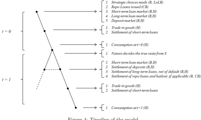
Figure 4: Timeline of the model
B: Bank, LoLR: Lender of Last Resort, CB: Central Bank, H: Households
2.5 Timing
There are five markets that convene at each time period t∈ T. The short-term (intraperiod) loan, long-term (interperiod) loan, deposit, and repo loan markets meet at the beginning of each time period, and the goods market meets subsequently in each period. As in Goodhart et al. (2010), this setup is chosen because it “maximizes the number of transactions possible and allows households to borrow in the short-term money market in order to invest in long-term bond or asset markets. It also allows for an explicit speculative motive for holding money.” A timeline of the model is provided in Figure 4.
2.6 Decision variables and budget sets
We denote macro variables, which are determined in equilibrium and which each household takes as fixed, by η= (p,r, rd, ρ,¯r)∈RS
∗ + ×RS
∗
+ ×R+×R+×R+.
The vectors of householdα andβ’s decisions are denoted,σα ∈Σα(η) andσβ ∈Σβ(η), re-spectively. σα= (bα, qα, µα, dα, να)∈
RS+×R+×R+×R+×R+andσβ = (bβ,qβ,µβ,µ¯β,ν¯β,νβ)∈
R+×RS+×RS+×R+×RS+×RS+.
The vector of the commercial bank γ’s decisions is denoted σγ ∈ Σγ(η) where σγ = (πγ,mγ,m¯γ, µγd, µγR,νγ)∈RS
∗ + ×RS
∗
+ ×R+×R+×R+×RS+.
ps : Price of the good in state s∈S∗
rs : Short-term loan rate offered by the bank in states∈S∗ rd : Interest rate on deposits offered by the bank
ρ : Interest rate on repo loans offered by the central bank ¯
r : Long-term loan rate offered by the bank
bhs : Amount of money spent on goods by householdh∈ {α, β}in states∈S∗ qhs : Quantity of goods offered for sale by householdh∈ {α, β} in states∈S∗ µhs : Short-term borrowing by householdh∈ {α, β} in states∈S∗
νsh : Short-term loan repayment rate of householdh∈ {α, β} in states∈S∗ dα : Deposit by householdα att= 0
¯
µβ : Long-term borrowing by householdβ att= 0 ¯
νsβ : Long-term repayment rate of householdβ in states∈S ch : Coefficient of risk aversion of agent h∈H
θs : Probability of states∈S ch
s : Consumption of household h∈ {α, β} in states∈S∗ ehs : Goods endowment of householdh∈ {α, β}in states∈S∗ mhs : Monetary endowment of household h∈ {α, β} in states∈S∗
eγs,i : Monetary endowment of bankγin states∈S∗, under risk profilei∈ {H, L}
MCB : Money supply att= 0
MsCB : Money injection by the central bank in the short-term loan market in state
s∈S
τ : Borrowing rate at the discount window in case of a bailout
λs : Non-pecuniary penalty for defaulting on short-term loans in states∈S∗
¯
λs : Non-pecuniary penalty for defaulting on long-term loans in states∈S λDs : Non-pecuniary penalty for defaulting on deposits in states∈S
πγ0 : Bank profits att= 0
mγs : Short-term loan extension by the bank in state s∈S∗
¯
mγ : Long-term loan extension by the bank att= 0
µγR : Amount borrowed by the bank via repo loans at t= 0
µγd : Amount borrowed by the bank via deposits att= 0
νsγ : Bank’s repayment rate on deposits in states∈S∗ cγ0 : Bank’s retained earnings att= 0
2.7 Agents’ behaviour
2.7.1 Household α
Householdα maximizes its utility from the consumption of the good in each period, and across each state of nature. Endowed with relatively more of the good at t = 0 than at t = 1, and
with cash, it smoothes consumption by selling part of its endowment at t= 0 and depositing part of its wealth with the commercial bankγ. In the second period, it uses its wealth to buy some of the consumption good.
Agentα’s optimization problem is as follows max σα∈Σ α Πα={u(cα0)−λ0max[0,(1−ν0α)µα0]}+ X s∈S θsu(cαs) s.t. Bα(η) ={σα∈Σα(η) : (01α)−(s1α)}
Agentα faces the following constraints: (01α) dα ≤ µ α 0 1 +r0 +mα0 (02α) µα0ν0α≤p0q0α (s1α) bαs ≤dα(1 +rd)νsγ+mαs
(01α) says that in the beginning oft = 0, household α borrows short-term and deposits these funds along with its monetary endowment for use in t= 1.
(02α) says that at the end oft= 0, household α repays the short-term loan using the proceeds of good sales.
(s1α) says that at the beginning of each states∈S, householdαuses the returns on its deposits and its monetary endowment to purchase the good.
Note that household α cannot sell more than its endowment and therefore q0α ≤eα0. θs is the
probability of state s occurring, cα
0 = (eα0 −q0α) is household α’s consumption in state 0 and cαs = (eαs +bαs
ps) is householdα’s consumption in states∈S.
2.7.2 Household β
Householdβ is endowed with relatively more of the good att= 1 than att= 0, and with cash. In order to smoothe consumption, it takes on an interperiod loan from the bankγ to buy some of the consumption good at t= 0. In the second period, it sells some of its endowment to pay
back part of its loan.
Household β’s optimization problem is as follows max σβ∈Σ β Πβ =u(cβ0) +X s∈S θs{u(cβs)−λ¯smax[0,(1−ν¯sβ)¯µβ]−λsmax[0,(1−νsβ)µβs]} s.t. Bβ(η) ={σβ ∈Σβ(η) : (01β)−(s2β)}
Household β faces the following constraints: (01β) bβ0 ≤ µ¯ β 1 + ¯r +m β 0 (s1β) µ¯βν¯sβ ≤ µ β s 1 +rs +mβs (s2β) µβsνsβ ≤psqβs
(01β) says that in t = 0, household β takes out a long-term loan and uses this along with its monetary endowment to purchase the consumption good.
(s1β) says that at the beginning of each states ∈S, household β repays some fraction of the long-term loan using short-term borrowings and irs monetary endowment.
(s2β) says that at the end of each state s∈ S, household β repays the short-term loan using the proceeds of good sales.
Note that householdβcannot sell more than its endowment and thereforeqβ
s ≤eβs.c β 0 = (e β 0+ bβ0 p0)
is household β’s consumption in state 0 and cβs = (eβs −qsβ) is household β’s consumption in state s∈ S. Its utility in state s∈ S is subject to a default penalties which are linear in the amount defaulted.
2.7.3 Commercial bank γ
The commercial bankγ is risk averse and maximizes expected utility of profits in both periods. It has quadratic preferences over profits i.e. it faces a portfolio allocation problem wherein it tries to diversify idiosyncratic risk. It borrows from depositors and from the central bank via a repo loan collateralized by its future monetary endowment. It uses these funds to extend short term liquidity in both periods and extend long-term credit via an interperiod loan. It faces a shock in monetary endowment that may make it illiquid in the bad state of nature, forcing it to default on its repo loan obligation. Depending on the realization of this shock and the policy stance of the LoLR, which is unknown to it, the commercial bank γ solves one of the following
three optimization problems.
The commercial bankγ’s optimization problem is as follows (a) No Default Case
max σγ∈ΣγΠ γ ={πγ 0 −cγ(π γ 0)2}+ X s∈S θs{πγs −cγ(πsγ)2−λDsmax[0,(1−νsγ)µ γ d]} s.t. Bγ(N D)(η) ={σγ ∈Σγ(η) : (01γ)−(s2γ)}
In this case, the commercial bankγ faces the following constraints: (01γ) mγ0+ ¯mγ≤ µ γ d 1 +rd + µ γ R 1 +ρ +e γ 0 (02γ) π0γ ≤mγ0(1 +r0)ν0α
LetSγ ⊆S denote all the states where the bank is solvent on its repo loan, i.e.
eγs > µγR ∀s∈Sγ
In the No Default case,Sγ=S and therefore the bank’s second period budget constraints are:
(s1γ) mγs +µγdνsγ+µγR≤∆(02γ) + ¯mγ(1 + ¯r)¯νsβ+eγs
(s2γ) πsγ≤mγs(1 +rs)νsβ
(01γ) says that int= 0, the commercial bankγ borrows from depositors and from the Central Bank, via a repo loan, and this combined with its monetary endowment is used to fund short-term and long-short-term loan offerings. The bank’s monetary endowment (which may be thought of as its other assets) is used as collateral for the repo loan taken from the Central Bank.
(02γ) says that at the end oft= 0, the commercial bankγ keeps short-term loan repayment as profit.
(s1γ) says that at the beginning of each states∈S, where the value of bank’s monetary endow-ment is greater than that of the repo loan repayendow-ment, bank γ uses long term loan repayment, its monetary endowment in states, and the cash carried over from the first period (∆(02γ)) to pay back depositors and the Central Bank, and issue short-term loans in states.
(s2γ) says that at the end of each state s∈S, bank γ keeps the short-term loan repayment as profit.
(b) Bailout Case max σγ∈Σ γ Πγ ={πγ0 −cγ(π0γ)2}+X s∈S θs{πγs −cγ(πsγ)2−λDsmax[0,(1−νsγ)µ γ d]} s.t. Bγ(DB)(η) ={σγ∈Σγ(η) : (01γ)−(s2γ)(DB)}
In this case, the commercial bankγ faces the following constraints: (01γ) mγ0 + ¯mγ≤ µ γ d 1 +rd + µ γ R 1 +ρ +e γ 0 (02γ) π0γ ≤mγ0(1 +r0)ν0α
For all statess∈Sγ the bank’s second period budget constraints are: (s1γ) mγs +µγdνsγ+µγR≤∆(02γ) + ¯mγ(1 + ¯r)¯νsβ+eγs
(s2γ) πsγ≤mγs(1 +rs)νsβ
For all statess /∈Sγ the bank’s second period budget constraints are:
(s1γ)(DB) mγs+µγdνsγ≤∆(02γ) + ¯mγ(1 + ¯r)¯νsβ+ µ γ B 1 +τ (s2γ)(DB) πγs ≤mγs(1 +rs)νsβ−µ γ B
(01γ) says that int= 0, the commercial bankγ borrows from depositors and from the Central Bank, via a repo loan, and this combined with its monetary endowment is used to fund short-term and long-short-term loan offerings. The bank’s monetary endowment (which may be thought of as its other assets) is used as collateral for the repo loan taken from the Central Bank.
(02γ) says that at the end oft= 0, the commercial bankγ keeps short-term loan repayment as profit.
(s1γ) says that at the beginning of each state s ∈ Sγ, where the value of bank’s monetary endowment is greater than that of the repo loan repayment, bank γ uses long term loan re-payment, its monetary endowment in state s, and the cash carried over from the first period (∆(02γ)) to pay back depositors and the Central Bank, and issue short-term loans in states. (s2γ) says that at the end of each states∈Sγ, bankγ keeps the short-term loan repayment as profit.
(s1γ)(DB) says that at the beginning of each state s /∈Sγ, where the value of bank’s monetary endowment is lower than that of the repo loan repayment, bankγ defaults on its repo loan but is bailed out and allowed to borrow from the discount window at an interest rate τ and uses this default window borrowing along with long term loan repayment, and the cash carried over from the first period to pay back depositors and to issue short-term loans in state s.
to repay the discount window borrowing (in full) and keeps the rest as profit. (c) No Bailout Case max σγ∈Σ γ Πγ={π0γ−cγ(πγ0)2}+ X s∈Sγ θs{πsγ−cγ(πγs)2−λDs max[0,(1−νsγ)µ γ d]} s.t. Bγ(DN)(η) ={σγ ∈Σγ(η) : (01γ)−(s2γ)}
The commercial bank γ faces the following constraints: (01γ) mγ0 + ¯mγ ≤ µ γ d 1 +rd + µ γ R 1 +ρ +e γ 0 (02γ) πγ0 ≤mγ0(1 +r0)ν0α
For all states s∈Sγ the bank’s second period budget constraints are: (s1γ) mγs +µγdνsγ+µγR≤∆(02γ) + ¯mγ(1 + ¯r)¯νsβ +eγs
(s2γ) πsγ≤mγs(1 +rs)νsβ
(01γ) says that int= 0, the commercial bankγ borrows from depositors and from the Central Bank, via a repo loan, and this combined with its monetary endowment is used to fund short-term and long-short-term loan offerings. The bank’s monetary endowment (which may be thought of as its other assets) is used as collateral for the repo loan taken from the Central Bank.
(02γ) says that at the end oft= 0, the commercial bankγ keeps short-term loan repayment as profit.
(s1γ) says that at the beginning of each state s ∈ Sγ, where the value of bank’s monetary endowment is greater than that of the repo loan repayment, bank γ uses long term loan re-payment, its monetary endowment in state s, and the cash carried over from the first period (∆(02γ)) to pay back depositors and the Central Bank, and issue short-term loans in states. (s2γ) says that at the end of each state s∈ Sγ, bank γ keeps the short-term loan repayment as profit. Since the bank rationally expects not to be bailed out if it defaults, its maximization problem is restricted to the states s∈Sγ. In this case, when the bank defaults on its repo loan (i.e. ins /∈Sγ), the Central Bank seizes the collateral and hands over all remaining bank assets to depositors who are the senior creditors. We assume costless liquidation of the bank’s assets. The depositors have to therefore take a haircut on their deposits. The effective repayment rate on deposits for the states s /∈Sγ is therefore defined as,νsγ = ∆(02γ)+ ¯mγ(1+¯r)¯νsβ
µγd ∀s /∈S γ.
2.8 Market clearing conditions
Each of the five markets in the model clears at a price that balances supply and demand in equilibrium. The market clearing conditions are:
(M C1) p0 = bβ0 q0α (M C2) ps= bα s qα s , ∀s∈S (M C3) (1 +r0) = µα0 mγ0 (M C4) (1 +rs) = µβs (mγs +MsCB) , ∀s∈S (M C5) (1 + ¯r) = ¯ µβ ¯ mγ (M C6) (1 +rd) = µγd dα (M C7) (1 +ρ) = µγR MCB
(M C1) and (M C2) say that in each states∈S∗ the goods market clears when the amount of
money offered for the good is exchanged for the quantity of the good offered for sale.
(M C3) says that at t = 0 the short-term loan market clears when the amount of short-term
credit demanded by households is exchanged for the amount of short-term credit offered by the bank.
(M C4) says that in each state s ∈ S the short-term loan market clears when the amount of
short-term credit demanded by households is exchanged for the amount of short-term credit offered by the bank and the amount injected by the central bank.
(M C5) says that the long-term loan market clears when the amount of long-term credit
de-manded by households is exchanged for the amount of long-term credit offered by the bank. (M C6) says that the deposit market clears when the amount of deposit borrowing demanded
by the bank is exchanged for the amount of deposits offered by households.
(M C7) says that the repo loan market clears when the amount of interbank borrowing demanded
by the bank is exchanged for the amount of money supplied by the central bank.
3
Equilibrium
There are two equilibrium concepts contained within this model – equilibrium in the strategic game, and a rational expectations equilibrium corresponding to each of the possible combina-tions of player accombina-tions. Their definicombina-tions and properties are explained below.
3.1 Definitions
3.1.1 Nash equilibrium
The mixed extension of the (finite) strategic game Γ =
N,(Ai)i∈N,(Fi)i∈N is the strategic game ˆΓ = N, ∆ (Ai)i∈N ,Fˆi i∈N
wherein ∆ (Ai) is the set of probability distributions over Ai, and for each α∈ ×j∈N∆ (Aj), ˆFi(α) =Pa∈A
Q
j∈Nαj(aj)
Fi(a).
The mixed strategy Nash equilibrium of the strategic game Γ =
N,(Ai)i∈N,(Fi)i∈N
is the Nash equilibrium of its mixed extension ˆΓ =
N, ∆ (Ai)i∈N ,Fˆi i∈N
. For the game defined in this paper, it is therefore a distribution over a profile of actionsα∗ ∈∆ (Aγ)×∆ (ACB) with
the property that for every player-typei∈N,every pure strategy in the support of αi∗ is a best response to α∗−i.
3.1.2 Monetary equilibrium with commercial banks, default, and the lender of last resort
Based on the strategic choices of the Bank and the LoLR, one of three possible equilibria attains. We say that (η,(σh)h∈H)(xx),(xx)∈ {N D, DB, DN} is a monetary equilibrium with
commercial banks, default, and the lender of last resort (MEBDL) iff:
(1) σα∈ arg max σα∈Bα(η) Πα (2) σβ ∈ arg max σβ∈Bβ(η) Πβ (3) σγ ∈ arg max σγ∈Bγ(xx)(η) Πγ, (xx)∈ {N D, DB, DN} (4) Equations (M C1) – (M C7) hold
Conditions (1), (2) and (3) ensure optimizing behaviour by both households and the com-mercial bank, and condition (4) implies that all markets clear. An equilibrium is therefore characterized by market clearing, rational expectations (i.e. correct anticipation of current and future prices, interest rates and repayment rates) and by agents optimizing within their budget sets.
3.2 Properties
3.2.1 Properties of the Nash equilibrium
The simultaneous game between the Bank and Central Bank has no pure strategy Nash equi-librium, so long as we have:
ΠγDB >ΠγN D>ΠγDN ΠCBDN >ΠCBDB
and, ΠCBN B >ΠCBN N
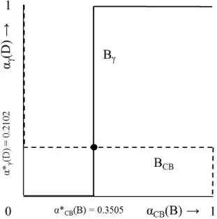
Allowing for mixed strategies, the bank is indifferent between Defaulting or Not Defaulting if the Central Bank plays a mixed strategy wherein it chooses to Bailout with probability
α∗CB(B) = (Π γ N D−Π γ DN) (ΠγDB−ΠγDN)
Similarly, the Central Bank would be indifferent between Bailing out or not if the bank plays a mixed strategy wherein it chooses to default with probability
α∗γ(D) = (Π
CB
N B−ΠCBN N)
(ΠCBDN −ΠCBDB) + (ΠCBN B−ΠCBN N)
We therefore have the mixed strategy Nash equilibrium α∗ ∈ ∆ (Aγ)×∆ (ACB) in the game
Γ = N,(Ai)i∈N,(Fi)i∈N with: Action sets: Aγ ={Default (D), No Default (N D)} ACB ={Bailout (B), No Bailout (N B)} Probability distributions: α∗(Aγ) = ( (ΠCBN B−ΠCBN N) (ΠCB DN −ΠCBDB) + (ΠCBN B−ΠCBN N) , (Π CB DN−ΠCBDB) (ΠCB DN −ΠCBDB) + (ΠCBN B−ΠCBN N) ) α∗(ACB) = ( (ΠγN D−ΠγDN) (ΠγDB−ΠγDN), (ΠγDB−ΠγN D) (ΠγDB−ΠγDN) )
3.2.2 Properties of the MEBDL
The following properties of the monetary equilibrium with commercial banks, default, and the lender of last resort hold. The existence of a local, stable equilibrium is proved numerically (see appendix). The formal proofs of the properties follow directly from Tsomocos (2003).
Relative Structure of Interest Rates The relative structure of interest rates is affected by the credit extension of banks and by default by agents. Overall liquidity in the model affects interest rates because it is a finite horizon model and fiat money must exit the system in the final period. Both inside and outside money therefore exit the system in the final period through loan repayments from households to banks and banks to the central bank. Default emerges as an equilibrium phenomenon affecting interest rates because the interest rates that clear the different debt markets price in the corresponding expected repayment rates through rational expectations.
Monetary Policy Non-Neutrality Given the presence of outside money in the model and default in debt markets, we have positive nominal interest rates ensuing since fiat money has a positive value and price. This value is derived from the role of money in facilitating all trans-actions, enforced through the cash-in-advance constraint. This also highlights the importance of liquidity.
The Quantity Theory of Money This model has a non-trivial quantity theory of money. Nominal changes affect both prices and quantities and therefore have a real effect. In each state
s∈S, nominal income equals the total money stock since all the liquidity available is pushed through to the goods market.
The Fisher Effect Nominal period interest rates are approximately equal to real inter-est rates plus expected inflation and a risk premium.
4
Calibration
Henceforth, we limit our discussion to a calibration of the model. First, for each possible combi-nation of strategic choices of the commercial bank and the LoLR, we compute the (competitive) monetary equilibrium attained across households and the commercial bank in our calibrated model. Subsequently, given the payoffs based on the computed monetary equilibria, we solve for the Nash equilibrium of the strategic game between the commercial bank and the LoLR.
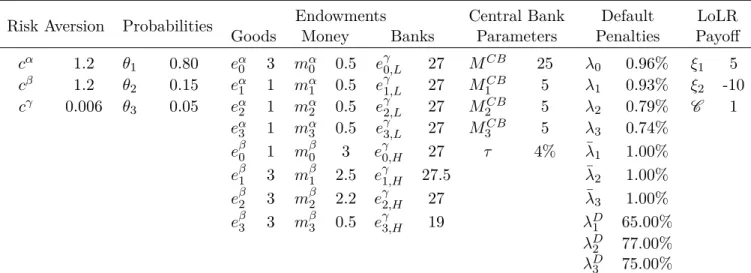
The exogenous variables used for the calibration of the economy are summarised below in Table 1. The parameters are chosen to clearly illustrate the effects of the ex ante strategic
0.8 and 0.15 respectively, and a ‘bad’ state with probability 0.05. Agentαis modelled as being relatively wealthier in the first period and therefore a net lender, whereas agent β is relatively wealthier in the second period and is therefore a net borrower. The exogenous risk profiles of the bank eγs,i, s ∈ S, i ∈ {H, L} are chosen such that they have the same expected value but differ significantly in riskiness. The high risk profile carries substantial tail risk, with a large reduction in value in the bad state of nature, while the low risk profile is risk free. Default penalties are chosen to allow for partial repayment (i.e. an intermediate level of default) in all states, to clearly observe changes across the different monetary equilibria.
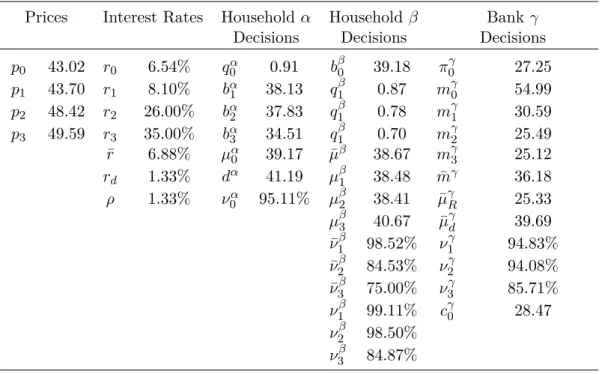
Tables 2, 3, and 4 summarise the values of decision variables and prices that attain at the No Default, Default & Bailout, and Default & No Bailout monetary equilibrium, respectively. To allow for an appropriate comparison of the different equilibria, the exogenous variables used in all three monetary equilibria are the same except for exogenous risk profiles of the bank
eγs,i, s ∈S, i ∈ {H, L} which differ based on the strategic choice of the bank. The No Default monetary equilibrium is realised when the bank chooses the low risk (riskless) profile, and results in the bank being solvent in all states of nature. The monetary endowments of the bank in this equilibrium are set to beeγs,L, s∈S. From the point of view of the bank (and the other agents), the No Default & No Bailout monetary equilibrium is identical to the No Default & Bailout monetary equilibrium, hence we have only one calibration. In the Default monetary equilibria, the only exogenous parameters that are different to the No Default monetary equilibrium are the monetary endowments of the bank which are now set to the high risk profile i.e. eγs,H, s∈S. Apart from the change in exogenous parameters, as described in Section 2.7 the budget sets and choice sets of the agents are different based on the stance of the LoLR assumed.
Table 1: Exogenous variables
Risk Aversion Probabilities Endowments Central Bank Default LoLR
Goods Money Banks Parameters Penalties Payoff
cα 1.2 θ1 0.80 eα0 3 mα0 0.5 e γ 0,L 27 MCB 25 λ0 0.96% ξ1 5 cβ 1.2 θ2 0.15 eα1 1 mα1 0.5 e γ 1,L 27 M1CB 5 λ1 0.93% ξ2 -10 cγ 0.006 θ3 0.05 eα2 1 mα2 0.5 e γ 2,L 27 M2CB 5 λ2 0.79% C 1 eα3 1 mα3 0.5 e3γ,L 27 M3CB 5 λ3 0.74% eβ0 1 mβ0 3 eγ0,H 27 τ 4% λ¯1 1.00% eβ1 3 mβ1 2.5 eγ1,H 27.5 λ¯2 1.00% eβ2 3 mβ2 2.2 eγ2,H 27 λ¯3 1.00% eβ3 3 mβ3 0.5 eγ3,H 19 λD1 65.00% λD2 77.00% λD 3 75.00% ch : Coefficient of risk aversion of householdh∈H
θs : Probability of states∈S
ehs : Goods endowment of householdh∈ {α, β}in state s∈S∗ mhs : Monetary endowment of household h∈ {α, β} in states∈S∗
eγs,i : Monetary endowment of bank γ in states∈S∗, under risk profile i∈ {H, L}
MCB : Money supply at t= 0
MsCB : Money injection by the central bank in the short-term loan market in states∈S τ : Borrowing rate at the discount window in case of a bailout
λs : Non-pecuniary penalty for defaulting on short-term loans in state s∈S∗
¯
λs : Non-pecuniary penalty for defaulting on long-term loans in states∈S λDs : Non-pecuniary penalty for defaulting on deposits in states∈S
Table 2: Monetary equilibrium values, No Default (ND) Prices Interest Rates Household α Household β Bank γ
Decisions Decisions Decisions
p0 43.02 r0 6.54% q0α 0.91 b β 0 39.18 π γ 0 27.25 p1 43.70 r1 8.10% bα1 38.13 q β 1 0.87 m γ 0 54.99 p2 48.42 r2 26.00% bα2 37.83 q β 1 0.78 m γ 1 30.59 p3 49.59 r3 35.00% bα3 34.51 q β 1 0.70 m γ 2 25.49 ¯ r 6.88% µα0 39.17 µ¯β 38.67 mγ3 25.12 rd 1.33% dα 41.19 µβ1 38.48 m¯γ 36.18 ρ 1.33% ν0α 95.11% µβ2 38.41 µ¯γR 25.33 µβ3 40.67 µ¯γd 39.69 ¯ ν1β 98.52% ν1γ 94.83% ¯ ν2β 84.53% ν2γ 94.08% ¯ ν3β 75.00% ν3γ 85.71% ν1β 99.11% cγ0 28.47 ν2β 98.50% ν3β 84.87%
ps : Price of the good in state s∈S∗
rs : Short-term loan rate offered by the bank in states∈S∗
¯
r : Long-term loan rate offered by the bank
rd : Interest rate on deposits offered by the bank
ρ : Interest rate on repo loans offered by the central bank
qh
s : Quantity of goods offered for sale by householdh∈ {α, β} in states∈S∗ bhs : Amount of money spent on goods by householdh∈ {α, β}in states∈S∗ µhs : Short-term borrowing by householdh∈ {α, β} in states∈S∗
νh
s : Short-term loan repayment rate of householdh∈ {α, β} in states∈S∗ dα : Deposit by householdα att= 0
¯
µβ : Long-term borrowing by householdβ att= 0 ¯
νβ
s : Long-term repayment rate of householdβ in states∈S πγ0 : Bank profits att= 0
mγs : Short-term loan extension by the bank in state s∈S∗
¯
mγ : Long-term loan extension by the bank att= 0
µγR : Amount borrowed by the bank via repo loans att= 0
µγd : Amount borrowed by the bank via deposits att= 0
νsγ : Bank’s repayment rate on deposits in states∈S∗ cγ0 : Bank’s retained earnings att= 0
Table 3: Monetary equilibrium values, Default & Bailout (DB) Prices Interest Rates Household α Household β Bank γ
Decisions Decisions Decisions
p0 42.98 r0 6.16% q0α 0.91 b β 0 39.06 π γ 0 27.25 p1 43.52 r1 8.10% bα1 37.66 q β 1 0.87 m γ 0 55.06 p2 47.86 r2 26.00% bα2 36.36 q β 1 0.76 m γ 1 30.45 p3 49.95 r3 35.00% bα3 35.48 q β 1 0.71 m γ 2 25.05 ¯ r 7.11% µα0 39.12 µ¯β 38.62 mγ3 29.11 rd 1.13% dα 41.00 µβ1 38.32 m¯γ 36.06 ρ 7.09% ν0α 95.26% µβ2 37.86 µ¯γR 26.77 µβ3 46.05 µ¯γd 39.56 ¯ ν1β 98.25% ν1γ 93.93% ¯ ν2β 83.49% ν2γ 90.64% ¯ ν3β 74.79% ν3γ 88.41% ν1β 98.28% cγ0 28.44 ν2β 96.05% µγB 7.04 ν3β 77.04%
ps : Price of the good in state s∈S∗
rs : Short-term loan rate offered by the bank in states∈S∗
¯
r : Long-term loan rate offered by the bank
rd : Interest rate on deposits offered by the bank
ρ : Interest rate on repo loans offered by the central bank
qh
s : Quantity of goods offered for sale by householdh∈ {α, β} in states∈S∗ bhs : Amount of money spent on goods by householdh∈ {α, β}in states∈S∗ µhs : Short-term borrowing by householdh∈ {α, β} in states∈S∗
νh
s : Short-term loan repayment rate of householdh∈ {α, β} in states∈S∗ dα : Deposit by householdα att= 0
¯
µβ : Long-term borrowing by householdβ att= 0 ¯
νβ
s : Long-term repayment rate of householdβ in states∈S πγ0 : Bank profits att= 0
mγs : Short-term loan extension by the bank in state s∈S∗
¯
mγ : Long-term loan extension by the bank att= 0
µγR : Amount borrowed by the bank via repo loans att= 0
µγd : Amount borrowed by the bank via deposits att= 0
νsγ : Bank’s repayment rate on deposits in states∈S∗ cγ0 : Bank’s retained earnings att= 0
µγB : Additional funds borrowed by the bank at the discount window when bailed out att= 1
Table 4: Monetary equilibrium values, Default & No Bailout (DN) Prices Interest Rates Household α Household β Bank γ
Decisions Decisions Decisions
p0 42.92 r0 1.94% qα0 0.91 b β 0 38.90 π γ 0 30.38 p1 42.72 r1 8.10% bα1 35.55 q β 1 0.83 m γ 0 55.16 p2 47.25 r2 26.00% bα2 34.75 q β 1 0.74 m γ 1 29.72 p3 184.63 r3 542.28% bα3 32.11 q β 1 0.17 m γ 2 24.50 ¯ r 0.87% µα0 39.07 µ¯β 38.57 m¯γ 35.90 rd 0.87% dα 39.32 µβ1 37.53 µ¯ γ R 25.22 ρ 7.42% ν0α 98.95% µβ2 37.17 µ¯γd 39.41 µβ3 32.11 ν1γ 88.94% ¯ ν1β 96.51% ν2γ 86.91% ¯ ν2β 82.20% cγ0 25.27 ¯ ν3β 16.45% ν1β 94.72% ν3γ 80.22% ν2β 93.49% ν3β 100%
ps : Price of the good in state s∈S∗
rs : Short-term loan rate offered by the bank in states∈S∗
¯
r : Long-term loan rate offered by the bank
rd : Interest rate on deposits offered by the bank
ρ : Interest rate on repo loans offered by the central bank
qh
s : Quantity of goods offered for sale by householdh∈ {α, β} in states∈S∗ bhs : Amount of money spent on goods by householdh∈ {α, β}in states∈S∗ µhs : Short-term borrowing by householdh∈ {α, β} in states∈S∗
νh
s : Short-term loan repayment rate of householdh∈ {α, β} in states∈S∗ dα : Deposit by householdα att= 0
¯
µβ : Long-term borrowing by householdβ att= 0 ¯
νβ
s : Long-term repayment rate of householdβ in states∈S πγ0 : Bank profits att= 0
mγs : Short-term loan extension by the bank in state s∈Sγ
¯
mγ : Long-term loan extension by the bank att= 0
µγR : Amount borrowed by the bank via repo loans att= 0
µγd : Amount borrowed by the bank via deposits att= 0
νsγ : Bank’s repayment rate on deposits in states∈Sγ cγ0 : Bank’s retained earnings att= 0
As can be seen from the tables above, the No Default monetary equilibrium leads to stable prices and reasonable levels of default, with an expected drop in credit extension by the bank in the bad state of nature, and a subsequent increase in default levels. This effect is exacerbated in the two Default monetary equilibria since in this case the bad state is characterised by a significant drop in the bank’s monetary endowment. In the case of the Default & Bailout monetary equilibrium, the availability of bailout funds at the discount window allows the bank to borrow in the bad state and extend credit despite the shock in the value of its monetary endowment and this allows for prices to remain stable and at levels comparable to the no default monetary equilibrium. Default levels are slightly higher in this monetary equilibrium since the presence of the discount window in the bad state of nature is rationally expected by all agents and this allows for a shifting in consumption which increases the marginal benefit from defaulting in the good states, thereby increasing the default levels slightly. The Default & No Bailout monetary equilibrium is much starker in contrast to the other two. In this case the bank defaults in the third state and so credit extension in this state stems solely due to the liquidity injection by the central bank in short-term debt markets. Short term interest rates in this state therefore spike up and this precipitates default by householdβ in the long-term debt market. This reduces the value of the bank’s assets, which are seized by the central bank upon its default, and handed over to the senior creditors – depositors. The depositors therefore end up taking a haircut on their debt. The shortage in credit supply precipitated by the failure of the bank in the bad state also affects the goods market raising prices significantly in this state.
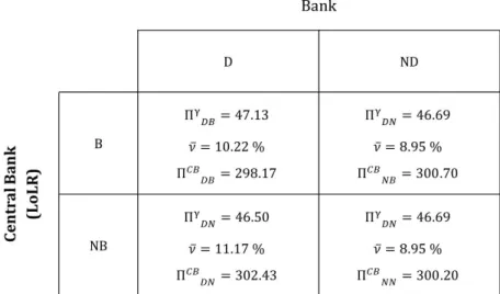
Figure 5: Payoffs of the two players in the strategic game
Figure 5 lists the payoffs for the two players given their strategic choices: Bailout (B) versus No Bailout (NB) choices for the LoLR, and Default (D) versus No Default (ND) choices for the bank. Figure 6 illustrates the mixed strategy Nash equilibrium, along with the best