A Two-Step Estimation Procedure and a Goodness-of-Fit Test for Spatial Extremes Models

(1)

Doctoral Dissertations University of Connecticut Graduate School

11-20-2013

A Two-Step Estimation Procedure and a

Goodness-of-Fit Test for Spatial Extremes Models

Hongwei Shang

University of Connecticut - Storrs, [email protected]

Follow this and additional works at:https://opencommons.uconn.edu/dissertations

Recommended Citation

Shang, Hongwei, "A Two-Step Estimation Procedure and a Goodness-of-Fit Test for Spatial Extremes Models" (2013).Doctoral

Dissertations. 256.

(2)

Goodness-of-Fit Test for Spatial Extremes

Models

Hongwei Shang, Ph.D. University of Connecticut, 2013

ABSTRACT

Parametric max-stable processes are increasingly used to model spatial extremes. Since the dependence structure is specified for block maxima, the data used for inference are block maxima from all sites. To improve the estimation efficiency, we propose a two-step approach with composite likelihood that utilizes site-wise daily records in addition to block maxima. Besides the parameter estimation, there is no formal model checking and diagnosis method for spatial extremes modeling yet. Model diagnosis in practice has been informal and mostly based on visual checking tools such as residual plot and quantile-quantile plot. We proposed a goodness-of-fit test for max-stable processes based on the comparison between a nonparametric and a parametric estimator of the corresponding unknown multivariate Pickands dependence function.

The proposed two-step procedure separates the estimation of marginal parameters and dependence parameters into two steps. The first step estimates the marginal pa-rameters with an independence Likelihood by ignoring the spatial dependence. Given

(3)

the marginal parameter estimates, the second step estimates the dependence parameters with a pairwise likelihood using block maxima. In a simulation study, the two-step ap-proach was found to provide more efficient estimator for the parameters and return levels than the composite likelihood approach based on block maxima data only. We applied the method to the maximum daily winter precipitation from 36 sites in California over 55 years, and compared with the composite likelihood approach.

A class of goodness-of-fit tests is proposed given the fact that the dependence struc-ture of a max-stable process is completely characterized by an extreme-value copula. The nonparametric estimators of the Pickands dependence function used in this work are those recently studied by Gudendorf and Segers. The parametric estimators rely

on the use of the pairwise pseudo-likelihood which extends the concept of composite

pairwise likelihood to a rank-based context. Approximate p-values for the resulting

margin-free tests are obtained by means of aone- or two-level parametric bootstrap. The

finite-sample performance of the tests is investigated in dimension 10 under the Smith, Schlather and geometric Gaussian models. An application of the tests to rainfall data is finally presented.

Key words: Extreme value analysis; Extreme-value copula; Extremal coefficient;

(4)

Goodness-of-Fit Test for Spatial Extremes

Models

Hongwei Shang

B.S., Applied Mathematics, Harbin Institute of Technology, Harbin, China, 2006 M.S., Management Science and Engineering, Harbin Institute of Technology, Harbin,

China, 2008

A Dissertation

Submitted in Partial Fulfillment of the Requirements for the Degree of

Doctor of Philosophy at the

University of Connecticut 2013

(5)

Copyright by

Hongwei Shang

(6)

APPROVAL PAGE

Doctor of Philosophy Dissertation

A Two-Step Estimation Procedure and a

Goodness-of-Fit Test for Spatial Extremes Models

Presented by Hongwei Shang, B.S., M.S. Major Advisor Jun Yan Associate Advisor Dipak K. Dey Associate Advisor Xuebin Zhang Associate Advisor Zhiyi Chi University of Connecticut 2013

(7)

Acknowledgements

I would like to send my deepest gratitude to my major advisor, Prof. Jun Yan, for his guidance, encouragement, and understanding during my graduate study. I am so lucky to have him as my advisor during my graduate studies. Prof. Yan led me to the interesting research field of spatial extremes. From Prof. Yan, not only had I learned knowledge and skills cruical for my career, but also learned how to solve problems and to work in a smart way. His enthusiasm towards research and his rigorous scientific attitude influence me deeply and set a good example for me. Prof. Yan, for all you have done that made me who I am today, I thank you deeply from my heart.

I would also like to thank my associate advisors Prof. Dipak Dey, Dr. Xuebin Zhang and Prof. Zhiyi Chi, for your guidance, useful discussions and thoughtful academic planning suggestions all through my graduate studies.

Especially, I thank Dr. Ivan Kojadinovic for giving valuable guidance in Chapter 5, including providing the theoretical support which makes the proposed approach theo-retically sound.

I would like to thank all the faculty, staff and my fellow graduate students in the Department of Statistics at the University of Connecticut for their support during my graduate study. Especially, I thank Prof. Ming-Hui Chen offering me an opportunity as a statistical consultant, from which I gained valuable experience. Many thanks to

(8)

my fellow graduate students in our department. Working with you smart people and developing friendship with you has been a joyful and unforgetable memory for me.

I also thank my English teachers Mary Romney and Anne Halbert during my first graduate year at University of Connecticut. Without their help, I would not have im-proved my English this fast and passed the speaking test within one year after arriving in the U.S..

I would like to thank the University of Connecticut Research Foundation and the Environment Canada. This research is partially supported by them.

Finally and most importantly, I would like to thank my family for their support and care. This thesis is dedicated to the memory of my mother Yuling Zhang. She is the greatest mother in the world, and I hope I can make her proud today. I want to also thank my father Yueming Shang, who is always loving and supportive even if we don’t get to meet very often because of the geographic distance. I also thank my husband Shaozhen Ma for his understanding and love. He is always there for me and supports me since we met back in 2003. I cannot imagine how my life would be without him. Finally, I want to thank our little angel Ethan, without whom I would have finished this dissertation one year earlier.

(9)

List of Tables

1 Parameter estimates and standard errors for each month with no trend. . 21

2 Estimated return levels and their 95% confidence intervals under different

choices for threshold u and run length r. . . 23

3 Parametric families of correlation functions. . . 34

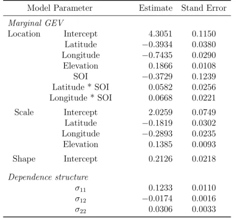
4 Summaries of parameter estimates and the standard errors. . . 45

5 Bias, empirical standard errors (ESE), average standard errors (ASE)

from sandwich estimators, and empirical coverage prabability (CP) of 95% confidence intervals for the model parameters (Par) from the two-step approach based on 1000 replicates for the geometric Gaussian model

with S = 25. . . 66

6 Bias, empirical standard errors (ESE), average standard errors (ASE)

from sandwich estimators, and empirical coverage prabability (CP) of 95% confidence intervals for the model parameters (Par) from the two-step approach based on 1000 replicates for the geometric Gaussian model

with S = 50. . . 67

7 Relative efficiency (%) in mean squared error of model parameter

es-timates for the pairwise likelihood approach using block maxima data

(13)

8 Relative efficiency (%) in MSE of joint and individual return levels (Joint,

s1, s2) for the pairwise likelihood approach using block maxima data

relative to the two-step approach. . . 70

9 Summaries of estimates (Est) and the standard errors (SE) for the model

parameters from two approaches (M1: composite pairwise likelihood

ap-proach using block maxima data; M2: two-step approach). . . 73

10 Marginal parameter estimates and the standard errors (SE) forM2

(two-step approach). . . 74

11 Joint 50-year return levels (cm) for three pairs at three different SOI

values based on both approaches (M1: pairwise likelihood approach using

block maxima data; M2: two-step approach). . . 84

12 Percentage of rejection ofH0 computed from 1000 samples of sizen

gen-erated from the models Sm–Iso, Sc–Exp and GG–Exp with parameter

valueθ for the p= 10 sites represented in the left plot of Figure 17. . . . 107

valueθ for the p= 10 sites represented in the middle plot of Figure 17. . 108

(14)

15 Summary of the max-stable models fitted to the Swiss rainfall data using

the SpatialExtremes R package. . . 111

16 Approximatep-values and execution times of the goodness-of-fit tests for

the max-stable models fitted to the Swiss rainfall data. The two lines for the model Sm–Ani correspond to the two- and the one-level parametric bootstrap, respectively. The timings are in hours and were obtained on a Linux machine with a 3.4GHz CPU. . . 113

(15)

List of Figures

1 Locations of the 192 monitoring stations in California superimposed with

the elevation map (100 meters). The sites in red are the 36 sites with full 55 years data from 1948 to 2002. The three sites in red triangles are

Napa, Winters, and Davis, near the Sacramento area. . . 7

2 Times series of daily precipitation at Debre Markos, Ethiopia. . . 16

3 Left: scatter plot of mean precipitation for each day overlaid with the

11-day moving average. Right: threshold chosen for each month. . . 17

4 Mean residual life plots with 95% confidence intervals (dashed lines) for

all months, r= 1. . . 19

5 95% confidence intervals for GEV parameters. Left: confidence intervals

forµ. Middle: confidence intervals forσ. Right: confidence intervals forξ. 21

6 Return levels (solid line) with 95% confidence intervals (dashed lines)

obtained from 5000 Monte Carlo simulation. The circles are the empirical

estimates based on the observed 53-year’s data. . . 23

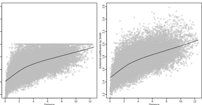
7 Nonparametric estimates of the extremal coefficients ζ for all possible

pairs of sites for the rainfall data. The left panel gives estimators based on Schlather and Tawn (2003), and the right panel gives estimators based

(16)

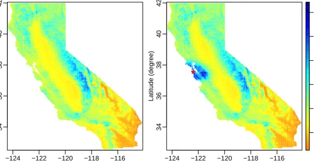
8 Return level maps when fixing SOI =−0.2175. Left: 50-year return levels (cm). Right: 50-year conditional return levels, conditioning on observing

an event of 15cm precipitation (35-year return level) at San Francisco. . . 48

9 Return period maps (in years) of 50-year return level after SOI value

changes. Left: the return period of a 50-year return level obtained with

maximum sample SOI (1.8775) when SOI actually takes the minimum

sample value (−3.1375). Right: the return period of a 50-year return

level obtained with minimum sample SOI (−3.1375) when SOI actually

takes the maximum sample value (1.8775). . . 50

10 Contour plot of the fitted extremal coefficient from the model as a function

of the difference in longitudes and latitudes of two sites. . . 51

11 Marginal parameter estimates at 36 sites. Upper left: intercepts in the

location parameter; upper right: SOI coefficients in the location param-eter; lower left: intercepts in the scale paramparam-eter; lower right: intercepts

in the shape parameter. . . 75

12 The standardized SOI efficients in the location parameters at 36 sites,

with all sites labeled. . . 76

13 Contour plot of the fitted pairwise extremal coefficient relative to a site

at San Francisco (denoted by an asterisk) based on the chosen geometric Gaussian model with isotropic dependence and exponential correlation

(17)

14 The scatterplot of madogram-based pairwise extremal coefficients with 100 bins versus the Euclidean distance; grey dots represent pairwise mado-gram, and black dots represent madogram with 100 bins. The curve is

the fitted extremal coefficient curve for the chosen max-stable model. . . 80

15 Comparison of empirical and model quantiles for annual maxima of groups

of sites. The sites used for each panel are shown in its map, and the outer band is a 95% overall confidence band and the inner one a 95% pointwise

confidence band obtained fromK = 5000 simulations. . . 81

16 The 50-year sample return levels (cm) for three pairs on the log scale.

Up-per: pairwise likelihood approach using block maxima data (M1); Lower:

two-step approach (M2). Left: Napa & Winters; Center: Napa & Davis;

Right: Winters & Davis. . . 85

17 The three different sets ofd= 10 sites used in the simulations. . . 104

18 The left (resp. middle, right) plot represents the graph of the precomputed

approximation of the mapping θ 7→ ζP,θ based on the CFG estimator for

each of the three models in the case of the set of sites represented in the left (resp. middle, right) plot of Figure 17. . . 124

(18)

19 The left (resp. middle, right) plot compares the graphs of the mappings based on closed-form expressions (solid lines) with those of the corre-sponding precomputed approximations (dashed lines) based on penalized splines for the Sm–Iso (resp. Sc–Exp, GG–Exp) model. The top (resp. middle, bottom) pair of curves correspondS to fictious sites at distance 1 (resp. 4, 8). . . 125

(19)

Chapter 1

Introduction

1.1

Introduction

Natural extremes have influential impact on not only the environment but also the hu-man society. For example, extreme temperature and precipitation have been associated with human health in both non-infectious and infectious diseases (Patz et al., 2003, 2005). Extreme data are often spatial in nature as data are recorded at a network of monitoring stations over time. Extreme weather and climate events may also exert spa-tial dependence because their occurrences are influenced by atmospheric circulation of very large spatial scale. Rare events that occur at multiple locations within a very short time interval can cause more damage, consume more resources, and demand stronger emergency management. For strategic emergency management and loss mitigation, un-derstanding spatial dependence and predicting risk events in a spatial context is needed. Although univariate extreme value modeling has been well developed (e.g., Coles, 2001), spatial extreme modeling has not gained sharpened focus until recently (e.g., de Haan and Pereira, 2006; Buishand et al., 2008; Padoan et al., 2010; Davison and Gholamrezaee, 2012). Two recent reviews are Davison et al. (2012) and Bacro and Gaetan (2012b),

(20)

with the latter focusing on spatial max-stable processes.

Max-stable processes are a class of spatial extremes models. A max-stable process extends the multivariate extreme value distribution to infinite dimension such that its every finite dimensional marginal distribution is a multivariate extreme value distribu-tion (de Haan, 1984). There are only a very limited number of parametric models for which statistical inference is viable for practical usage: the Smith model (Smith, 1990), the Schlather model (Schlather, 2002), the Brown–Resnick model (Kabluchko et al., 2009), and the geometric Gaussian model (Davison et al., 2012). Wadsworth and Tawn (2012) proposed to superimpose two max-stable processes to obtain a new model, which can produce more realistic event realizations than, for example, the Smith model by itself.

Although max-stable process is mathematically elegant, there is a space for further improvement from at least two aspects, model parameter estimation and model diagno-sis. Inferences for max-stable process models are challenging because the joint density is generally unavailable. Instead, only the bivariate marginal distributions are available for the aforementioned models except for the Smith model, for which the trivariate marginal distributions have been derived (Genton et al., 2011). Recent applications relied on the composite likelihood approach based on the bivariate marginal distributions of block maxima data (Padoan et al., 2010; Davison and Gholamrezaee, 2012); all the remaining daily information are completely discarded. For model diagnosis, current tests are only visual model checking with no test statistics. No formal goodness-of-fit test has been

(21)

developed for max-stable processes.

To address the disadvantages of pairwise likelihood-based inferences and to improve the parameter estimation efficiency, we propose a two-step approach that utilizes daily records in addition to block maxima from each site for max-stable process models. The first step estimates the marginal parameters using an independence likelihood con-structed from the univariate threshold-based point process approach with daily records. Given the marginal parameter estimates, the second step estimates the dependence pa-rameters from a pairwise likelihood with block maxima.

For model checking, the quality of the fit of a spatial model based on a parametric max-stable process have been essentially investigated by means of graphical tools. No formal goodness-of-fit tests have been developed for spatial models based on max-stable processes. The purpose of our work is to fill this gap. Starting from the fact that the dependence structure of a max-stable process is completely characterized by an extreme-value copula, we propose a class of goodness-of-fit tests based on the comparison between a nonparametric and a parametric estimator of extremal coefficients. The finite-sample performance of the tests is investigated under the Smith, Schlather and geometric Gaussian models.

(22)

1.2

Motivating Example—Extreme Winter

Precipi-tation in California

In this section we will present our motivating application with annual maximum winter

daily precipitation in California. Large sacle climate variability such as El Ni˜no/Southern

Oscillation (ENSO) have significant impacts on extreme precipitation in north Amer-ica (Zhang et al., 2010). Southern Oscillation refers to the variation in the sea surface temperature of the tropical waters in the eastern Pacific Ocean. The “warm” events

and the “cool” events are referred to as El Ni˜no and La Ni˜na, respectively, and their

strength is measured by the Southern Oscillation Index (SOI), the normalized sea level pressure difference between Tahiti and Darwin. Recently, Zhang et al. (2010) fit gener-alized extreme value (GEV) distribution to winter season maximum daily precipitation at a number of individual sites over North America with ENSO as a predictor in the parameters of the GEV distribution. They found that ENSO have spatially consistent

and statistically significant influences on extreme precipitation. For example, an El Ni˜no

is associated with a substantial increase in the likelihood of extreme precipitation over a vast region of southern North America. This suggests that when a higher value of extreme precipitation occurs at a site in a year, extreme precipitation at nearby sites in the same year may also be higher due to the influence of large scale circulation. This also indicates spatial dependency in extreme precipitation and as such, analyzing extreme precipitation at individual site independently such as fitting a separate GEV distribution

(23)

for each site as is done in Zhang et al. (2010) is not sufficient when assessing the risks of extreme precipitation over a region. The simultaneous or nearly- simultaneous occur-rence of extremes at multiple places will drastically increase the demand for emergency responses. Therefore, for the purpose of risk management and emergency preparedness, while it is important to ask questions like “what is the 50-yr return level for a city”, it is also very important to ask “what is the probability that the 50-yr return levels of three sites in the vicinity of a city occur in the same year?”

Daily precipitation records at all monitoring stations in California were extracted from the second version of the Global Historical Climatology Network (GHCN), com-piled and quality controlled at the National Climatic Data Center of the National

Oceanic and Atmospheric Administration (available at http://www.ncdc.noaa.gov/

oa/climate/ghcn-daily/). Raw data of daily rainfall observations at 230 sites are

available in California starting from 1878, but all sites have missing values. As most precipitations in California occur in winters, we restrict our attention to only the winter season, which is defined as the period from December 1st to March 31st in the following year (Zhang et al., 2010). We label this four months’ data the year which contributes the December data; for example, winter 1948 refers to the period from December 1948 to March 1949. Due to missing data, the block maxima in a given winter at a given site was considered to be a valid one only if no more than 10% missing daily records were missing in that winter (Shang et al., 2011). The data before 1948 were sparse with no more than 40 sites. The data we use consist of winter maximum daily precipitation

(24)

from 1948 to 2002 for 192 sites (Figure 1). Possible covariates are longitude, latitude, elevation, and SOI. The longitude and latitude are in degrees, and the elevation is in 100 meters. The SOI variable used in the analysis for each winter season is the average of the

four monthly SOI values of the winter months, ranging from −3.1375 to 1.8775 with a

sample average−0.152. In contrast to the other three variables, which are site-specific,

SOI is a season-specific variable. These variables can be incorporated into the

parame-ters of the marginal GEV distribution at all sites. The covariate vector at sites in year

t is X0(s, t) = {X1(s), X2(s), X3(s), X4(t)}, where X1 is latitude, X2 is longitude, and

X3 is elevation, and X4 is SOI. Latitude, longitude, and elevation are centered at the

values at San Francisco (−122.38, 37.62, 0.02). SOI is centered at the sample average

−0.152.

As a max-stable process model only specifies the dependence structure of the block maxima, all the remaining daily observations are wasted. A natural question is, can we take advantage of daily records and improve the efficiency of parameter estimators? This motivates our proposed two-step approach for making inference. If the proposed two-step approach can yield smaller standard errors for parameter estimates and tighter confidence regions for jointly defined risk measures than the existing approach based on block maxima only, the reduction in uncertainty in assessing the joint risks of extreme precipitation over a region will be crucial to public safety alert, evacuation management, and loss mitigation.

(25)

−124 −122 −120 −118 −116 34 36 38 40 longitude (degree) latitude (degree) ● ● ● ● ● ● ● ● ● ● ● ● ● ● ● ● ● ● ● ● ● ● ● ● ● ● ● ● ● ● ● ● ● ● ● ● ● ● ● ● ● ● ● ● ● ● ● ● ● ● ● ● ● ● ● ● ● ● ● ● ● ● ● ● ● ● ● ● ● ● ● ● ● ● ● ● ● ● ● ● ● ● ● ● ● ● ● ● ● ● ● ● ● ● _● ● ● ● ● ● ● ● ● ● ● ● ● ● ● ● ● ● ● ● ● ● ● ● ● ● ●● ● ● ● ● ● ● ● ● ● ● ● ● ● ● ● ● ● ● ● ● ● ● ● ● ● ● ● ● ● ● ● ● ● ● ● ● ● ● ● ● ● ● ● ● ● ● ● ● ● ● ● ● ● ● ●● ● ● ● ● ● ● ● ● ● ● ● 0 10 20 30 40

Figure 1: Locations of the 192 monitoring stations in California superimposed with the elevation map (100 meters). The sites in red are the 36 sites with full 55 years data from 1948 to 2002. The three sites in red triangles are Napa, Winters, and Davis, near the Sacramento area.

and a data example in extreme precipitation data in Ethiopia is presented in Chapter 2. Max-stable processes theory for spatial extremes, model inference and the dependence measure extremal coefficient are introduced in Chapter 3 with an application to winter maximum daily precipitation in California. Chapter 4 presents our proposed two-step approach. In this chapter, a simulation study is reported to assess the efficiency gain of two-step approach compared to current practice based on block maxima only and the two-step approach is applied to the winter precipitation data. Chapter 5 presents

(26)

our proposed goodness-of-fit testing procedures and demonstrates the performance via a simulation study. The last section in this chapter presents the application of the tests to the Swiss rainfall data analyzed in Davison et al. (2012). Chapter 6 concludes the thesis.

(27)

Chapter 2

Univariate Extreme-value Theory

2.1

Generalized Extreme Value Distribution

Extreme value theory has evolved into a proliferating field in statistics, motivated by numerous environmental applications. The main statistical approaches are fitting gen-eralized extreme-value distributions to maxima and fitting gengen-eralized Pareto distribu-tions or point processes to exceedences over high thresholds (Coles, 2001; Beirlant et al., 2004). This chapter reviews the basic theory and statistical methodology on univariate extremes, then presents a detailed analysis with daily time series of precipitation records at Debre Markos in the Northwestern Highlands of Ethiopia.

The GEV distribution was first introduced by Fisher and Tippett (1928) as limits of the sample maximum or minimum for independent, identically distributed variables.

LetY1,Y2, . . . be a sequence of independent and identically distributed random variables

with common distribution function G, the basis of extreme value modeling is the GEV

distribution for Mn = max{Y1, . . . , Yn}. If there exist sequences of constants {an > 0}

and {bn} such that

(28)

asn→ ∞for a non-degenerate distribution functionF, thenF is a member of the GEV family F(z;µ, σ, ξ) =          expn− 1 +ξ z−_σµ−1/ξo , ξ6= 0, 1 +ξ z−_σµ >0, exp −exp −z−µ σ , ξ= 0, (2.2)

where µ∈ _R is a location parameter, σ >0 is a scale parameter, and ξ ∈_R is a shape

parameter governing the tail behavior. The Gumbel family is the limiting case ofξ→0.

The sub-families defined by ξ > 0 and ξ <0 correspond to the Fr´echet family and the

Weibull family, respectively. The m-year return level zm, with the return period 1/m,

is calculated from F(zm) = 1−1/m.

2.2

Model Inference Approaches

2.2.1

Block Maxima Approach

This section reviews three main approaches in modeling univariate extreme values, in-cluding block maxima approach, the peaks over threshold (POT) approach (Balkema and de Haan, 1974; Pickands, 1975) and the point process approach (Pickands, 1971; Leadbetter et al., 1983). The GEV distribution provides a model for the distribution of block maxima. The model fitting for block maxima approach consists of choosing the block size and fitting the GEV distribution to the set of block maxima. The choice

(29)

of block size is a trade-off between bias and variance. In practice, the block is often chosen to be one year. To make inferences about the parameters in the GEV distribu-tion, the maximum likelihood approach can be applied. Usual regularity conditions of

the maximum likelihood estimator are satisfied whenξ >−0.5 (Smith, 1985). Note the

difficulty that the normalizing constants will be unknown in practice is easily resolved

by approximating the distribution ofMnby a different member of the same GEV family.

Without loss of generality, we assume an = 1 andbn= 0 here.

2.2.2

Peaks over Threshold Approach

One difficulty in the above extreme value analysis is the limited amount of data for model estimation. If the entire time series of observations are available, the POT approach is more attractive in that all exceedances over threshold, instead of just the block maxima, contribute to the inference. The POT approach is based on the conditional distribution

of exceedances over a thresholdu. LetY denote an arbitrary term in the{Yi}sequence.

For large enoughu, the probability that it exceeds by at leastv is {1−G(u+v)}/{1−

G(u)}. SupposeGsatisfies the same conditions as lead to (2.1), the distribution function

of (Y −u), conditional onY > u, is approximately H(v; ˜σ, ξ) = 1− 1 + ξv ˜ σ −1/ξ , v >0, (1 +ξv/σ˜)>0. (2.3)

(30)

This family of distributions is the generalized Pareto family. The parameters in (2.3)

are uniquely determined by those in (2.2). The parameter ξis the same as that in (2.3),

while ˜σ can be expressed by ˜σ=σ+ξ(u−µ) with µand σ in (2.2).

This POT approach considers exceedances by defining a high thresholdu. Although

the value of threshold can be arbitrary to some extent for initial analysis, too low a threshold is likely to violate the asymptotic basis of the model and too high a threshold will lead to too few exceedances for data analysis. The ideal threshold is determined

by considering the smallest u beyond which the parameter estimates stabilize. An

ex-ploratory tool for choosing u is the mean residual life plot (e.g., Coles, 2001, Ch.4).

When u is sufficiently large, the expected residual life, E(X −u|X > u), is a linear

function of u. After choosing the threshold, the parameters of the generalized Pareto

distribution can then be estimated by maximizing likelihood derived from (2.3).

Another approach is based on the behavior of several largest order statistics within a block; however, it could be wasteful if one block happens to contain more extreme events than another. Both characterizations can be unified using a point process representation discussed below.

2.2.3

Point Process Approach

The point process approach was originally introduced by Pickands (1971). Assuming that Y1, . . . , Yn are independent and identically distributed, Pickands (1971) showed

(31)

i = 1, . . . , n} is approximated by a Poisson process on the region (0,1)×[u,∞) with intensity function on A= (t1, t2)×[z,∞) given by

Λ(A) = ny(t2−t1) 1 +ξ z−µ σ −1/ξ , (2.4)

whereny is the number of blocks of data to which the availableYi correspond, ensuring

that the parameters (µ, σ, ξ) are the same as those in the GEV approximation (2.2) of

block maxima. Both the block maxima approach and POT approach can be derived

from this representation. Suppose that we observe k exceedances from a sequence of

observations over threshold u, y1, . . . , yk, from ny block’s of data. Regarding the

prob-ability of the observed data as a function of the unknown parameter, the likelihood derived from the Poisson process has the form

L(µ, σ, ξ;y1, . . . , yk) = exp ( −kny 1 +ξ u−µ σ −1/ξ) k Y i=1 σ−1 1 +ξ yi−µ σ −1/ξ−1 . (2.5)

The point process likelihood is based on all data greater thanu, thus inference are likely

to be more accurate than estimates based on the classical GEV model which studies only block maxima. The likelihood also takes into account of missing data in that where

there are missing data, ny will be the number of block’s worth of observed data.

(32)

identically distributed; however, for the daily series data to which extreme value mod-els are applied, this is usually an unrealistic asssumption. Environmental data tend to violate the assumpation in two aspects (Smith, 1989). First, daily data exhibit short-range dependence leading to clustering of exceedances over threshold; second, there exists non-stationarity possibly because of seasonal effects. To deal with the problem of dependent exceedances, the most widely-adopted method is declustering. It corre-sponds to filtering the dependent observations to obtain a set of threshold excesses that are approximately independent (Smith and Weissman, 1994). For a given threshold, a simple way of declustering is to define clusters to be wherever there are consecutive exceedances of this threshold. In particular, two exceedances of the threshold that are

separated apart by fewer thanr observations are deemed part of the same cluster. That

is, only after a certain number, r, of observations falls below the threshold, the cluster

is terminated. In practice, it is recommended to try different r values for comparison

(Smith, 1989; Mannshardt-Shamseldin et al., 2010). Another way to deal with the tem-poral dependence is to simply ignore it, recently proposed by Fawcett and Walshaw (2007). They showed that this approach not only uses all threshold excesses for more efficient estimation, but also avoids significant biases that may come with the decluster-ing approach (Fawcett and Walshaw, 2007, 2012). To handle the non-stationarity due to seasonal effects, a simple and practical approach of broad utility is to break up the year into a finite number of seasons and to fit separate GEV models within each season (Smith, 1989). It allows all model parameters to be seasonally dependent. Next section

(33)

we will apply these techniques to the extreme precipitation data in Ethiopia.

2.3

Application to Extreme Precipitation in Ethiopia

Understanding the extreme precipitation is very important for Ethiopia, which is heav-ily dependent on low-productivity rainfed agriculture but lacks structural and non-structural water regulating and storage mechanisms. There has been increasing con-cern about whether there is an increasing trend in extreme precipitation as the climate changes. Existing analysis of this region has been descriptive, without taking advantage of the advances in extreme value modeling. In this section, we present the first analysis of extremes of this region with daily time series of precipitation records at Debre Markos in the Northwestern Highlands of Ethiopia.

2.3.1

Data

Debre Markos is a city in the Blue Nile River basin on the Northwestern Highlands

of Ethiopia. It has latitude 10◦200N, longitude 37◦430E, and elevation 2446 meters.

Although the topography of Ethiopia is highly diverse, more than 45% of the country is dominated by highlands with elevations greater than 1500 meters, where almost 90% of the nation’s population resides. The rain gauge station at Debre Markos provides the longest record among all stations in Ethiopia. Daily precipitation records are available from 1953, with only a tiny proportion of missing data. We use Debre Markos as a case

(34)

Year Daily precipitation (mm) 1960 1970 1980 1990 2000 0 20 40 60 80

Figure 2: Times series of daily precipitation at Debre Markos, Ethiopia.

study to investigate the long term trend in extreme precipitation in the Northwestern highland of Ethiopia.

Our raw data of daily precipitation at Debre Markos spans from November 1, 1953 to December 10, 2006. Out of the total of 19,398 days, 229 (about 1.2%) observations are missing. The observed daily time series of precipitation is plotted in Figure 2. The maximum daily was 86.9mm, observed on August 14, 1997.

The daily precipitation series are obviously not independent and not identically dis-tributed. Larger precipitations may tend to occur in clusters. For instance, out of 76 days in Junes with precipitation exceeding the 95th percentile of June precipitation, there were 9 occasions of two or more consecutive exceedances. These counts are 7 out of 79, 3 out 78, and 7 out of 80 for July, August, and September, respectively, the other three most rainy months. If there were no temporal dependence, 5% of the exceedances would be expected to be followed by another exceedance. The relative frequencies of

(35)

Month A v er age Precipitation f or all y ears (mm) 1 2 3 4 5 6 7 8 9 10 12 0 2 4 6 8 10 ● ● ● ● ● ● ● ● ● ● ● ● 2 4 6 8 10 12 5 10 15 20 25 30 Month Threshold f or each month (mm)

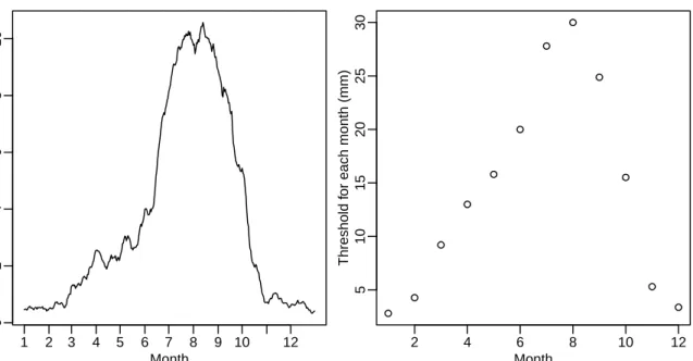
Figure 3: Left: scatter plot of mean precipitation for each day overlaid with the 11-day moving average. Right: threshold chosen for each month.

clustered exceedances are higher than 5%, which confirms that there is temporal depen-dence and hence the declustering is necessary.

Strong seasonality naturally exists in the data. As most areas in Ethiopia, there are three seasons in Debre Markos: main rainy season (June to September), dry season (October to January), and small rainy season (February to May), which are locally known as Kiremt, Bega, and Belg, respectively. Figure 3 (left panel) shows the mean precipitation for each day in a year, with the 11-day moving average overlaid. The plot is consistent with the three seasons. High precipitations are observed in summer months and low precipitations are observed in winter months. Our extreme value analysis needs to take the clustering and seasonality into account.

(36)

2.3.2

Results

Given the relatively short period of data record (53 years), the point process approach is adopted in this application as it takes full advantage of daily precipitation record in fitting GEV distributions. Before we apply the likelihood function, we remove the clustering and seasonality from the observed data as discussed in Section 2.2.3. For illus-tration, we use the traditional declustering method for solving the temporal dependence issue. Specifically, we allow each month to have its own GEV parameters as in Smith

(1989). Next, we need to select the threshold u. We plot the sample mean residual

life against threshold u in a mean residual life plot, and choose the smallest u beyond

which the mean residual life plot is approximately linear. Figure 4 shows the mean

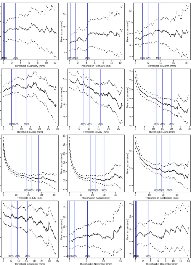
residual plots with 95% confidence intervals for each month with run length r = 1. For

all months, the figures are approximately linear when the threshold exceeds the sample 95% percentile. Therefore, we take the 95% percentile as threshold for each month. This is different from the analysis of Smith (1989), where the same threshold was used for all months. The right panel of Figure 3 shows the thresholds we choose for each month, which has similar pattern as the average precipitation plot in the left panel.

Each month is modeled separately, thus no specific form describing the seasonal

variation is assumed. Let µij, σij and ξij denote the GEV parameters for month j of

year i. To detect the long-term trend for each month, we assume the form

(37)

0 2 4 6 8 10 12 2 3 4 5 6 7 8 9 Threshold in January (mm) Mean e xcess (mm) 85%90% 95% 0 2 4 6 8 10 12 4 6 8 10 Threshold in February (mm) Mean e xcess (mm) 85% 90% 95% 0 5 10 15 20 4 6 8 10 12 Threshold in March (mm) Mean e xcess (mm) 85% 90% 95% 0 5 10 15 20 25 30 2 4 6 8 10 12 Threshold in April (mm) Mean e xcess (mm) 85%90% 95% 0 5 10 15 20 25 4 6 8 10 Threshold in May (mm) Mean e xcess (mm) 85% 90% 95% 0 5 10 15 20 25 30 2 4 6 8 10 12 14 Threshold in June (mm) Mean e xcess (mm) 85% 90% 95% 0 10 20 30 40 5 10 15 20 25 30 Threshold in July (mm) Mean e xcess (mm) 85%90% 95% 0 10 20 30 40 5 10 15 20 25 30 35 Threshold in August (mm) Mean e xcess (mm) 85%90% 95% 0 10 20 30 5 10 15 Threshold in September (mm) Mean e xcess (mm) 85% 90% 95% 0 5 10 15 20 25 30 35 4 6 8 10 12 14 Threshold in October (mm) Mean e xcess (mm) 85% 90% 95% 0 5 10 15 4 6 8 10 12 14 Threshold in November (mm) Mean e xcess (mm) 85%90% 95% 0 2 4 6 8 10 12 14 4 6 8 10 12 Threshold in December (mm) Mean e xcess (mm) 85%90% 95%

Figure 4: Mean residual life plots with 95% confidence intervals (dashed lines) for all

(38)

where the location parameterµij includes a linear trend in year with coefficientβj. This

form was also adopted to detect trend by Smith (1989) with ground-level ozone and

by Cooley (2009) with annual maximum temperatures. The likelihood Lj of month j,

j = 1, . . . ,12, is maximized separately to estimate (αj, βj, σj, ξj).

It turns out that none of theβj parameters is significant at 5% level, indicating there

is no strong evidence of long-term increasing trend over time. This means, for instance, that the 100-year return level has not increased significantly during the period of 1953—

2006. The models are re-fitted with all βj = 0. The sum of the minimized log likelihood

is−3063.91 for the models in all 12 months, which is very close to that with βj’s in the

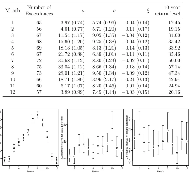
model (−3060.29). The parameter estimates with no trend are shown in Table 1. There

is strong seasonal pattern for the location parameter µ. The other parameters σ and

ξ, however, vary haphazardly. All ξ’s are estimated greater than −0.5, indicating that

the estimators are regular and they have the usual asymptotic properties. The 10-year return level for each specific month, calculated from GEV distribution, is also shown in the table.

The 95% confidence intervals for parameter estimates are calculated by profile likeli-hood (Coles, 2001, Ch.2), which is shown in Figure 5. Although the confidence interval

of ξ covers zero in all months, we do not reduce the model to the Gumbel model with

constraintξ = 0, because “a reduction to the Gumbel subfamily is always risky” (Coles

and Pericchi, 2003, p.416); the uncertainty in parameter ξ would otherwise be

(39)

Table 1: Parameter estimates and standard errors for each month with no trend.

Month Number of µ σ ξ 10-year

Exceedances return level

1 65 3.97 (0.74) 5.74 (0.96) 0.04 (0.14) 17.45 2 56 4.61 (0.77) 5.71 (1.20) 0.11 (0.17) 19.15 3 67 11.54 (1.17) 9.05 (1.35) −0.04 (0.12) 31.00 4 68 15.60 (1.20) 9.25 (1.38) −0.04 (0.12) 35.42 5 69 18.18 (1.05) 8.13 (1.21) −0.14 (0.13) 33.92 6 67 21.72 (0.88) 6.89 (1.01) −0.11 (0.11) 35.46 7 72 30.68 (1.12) 8.80 (1.23) −0.02 (0.11) 50.00 8 75 33.04 (1.12) 8.66 (1.34) 0.18 (0.14) 57.14 9 73 28.01 (1.21) 9.50 (1.34) −0.09 (0.12) 47.34 10 66 18.71 (1.80) 13.96 (2.17) −0.24 (0.13) 42.94 11 60 6.17 (1.07) 8.20 (1.46) 0.01 (0.14) 24.94 12 57 3.89 (0.99) 7.45 (1.44) −0.03 (0.15) 20.16 ● ● ● ● ● ● ● ● ● ● ● ● 2 4 6 8 10 12 5 10 15 20 25 30 35 Month Confidence Inter v al f or location par ameter (mm) ● ● ● ● ● ● ● ● ● ● ● ● ● ● ● ● ● ● ● ● ● ● ● ● 2 4 6 8 10 12 5 10 15 Month Confidence Inter v al f or scale par ameter ● ● ● ● ● ● ● ● ● ● ● ● ● ● ● ● ● ● ● ● ● ● ● ● 2 4 6 8 10 12 −0.4 −0.2 0.0 0.2 0.4 Month Confidence Inter v al f or shape par ameter ● ● ● ● ● ● ● ● ● ● ● ●

Figure 5: 95% confidence intervals for GEV parameters. Left: confidence intervals for

µ. Middle: confidence intervals forσ. Right: confidence intervals for ξ.

To check the sensitivity of results to the choice of threshold u and run length r,

return levels are compared under different choices. Since there is seasonality during the year, the calculation of the return level can be derived through the maxima for each

(40)

zm will satisfy 1− 1 m = Pr{max(M1, ..., M12)≤zm}= 12 Y i=1 exp ( − 1 +ξi zm−µi σi −1/ξi) . (2.7)

The confidence interval for return level can be obtained by simulation. We simulate the model parameters first from the the multivariate normal approximation of the estimator. For each set of generated parameters, a realization of the return level is obtained by

solving equation (2.7). A large number (N = 5000) of realizations is used to approximate

the confidence intervals.

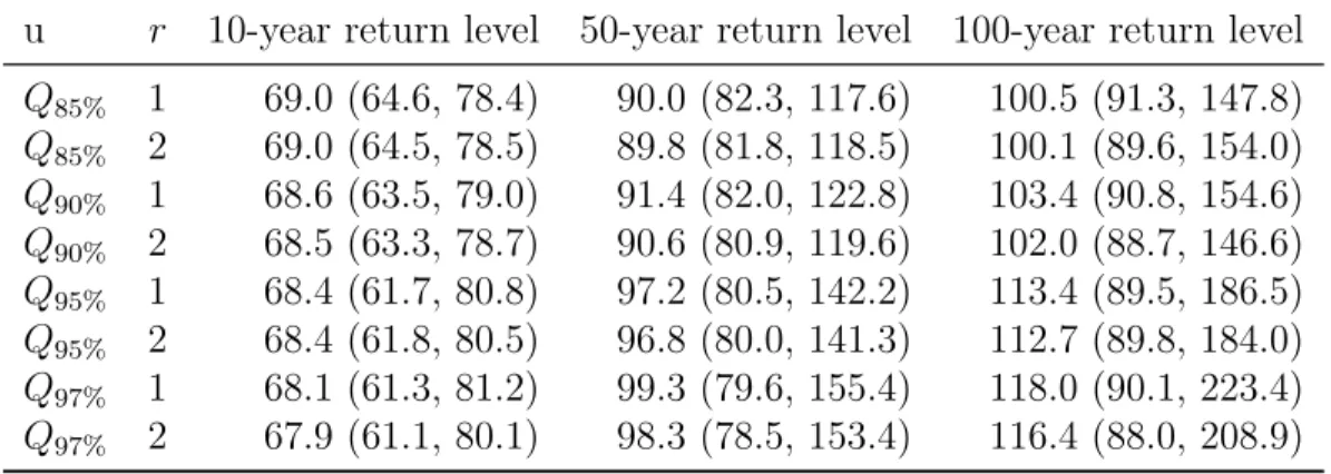
Table 2 summarizes the parameter estimates and 95% confidence intervals for 10-year,

50-year and 100-year return levels for different combinations of (u, r). It appears that

the inference is quite robust on the choice ofr for all return levels. The inference on the

10-year return level is robust to the choice ofu, but the 50-year and 100-year return levels

are less so, which is most evident from the upper bound of the 95% confidence interval. The change in confidence intervals is not completely surprising because the sample size

of exceedances decreases as u increases. With the confidence intervals in consideration,

the changes in the point estimate of return levels appear reasonably robust.

Among all those threshold sets, the only significant βj’s were found when u=Q90%

and r = 1, with standardized beta values −2.07 and −2.15 for February and July,

respectively. We conclude that there is no increasing long-term trend for any month. As a model diagnosis, we performed goodness-of-fit test for the GEV distribution

(41)

Table 2: Estimated return levels and their 95% confidence intervals under different

choices for threshold u and run length r.

u r 10-year return level 50-year return level 100-year return level

Q85% 1 69.0 (64.6, 78.4) 90.0 (82.3, 117.6) 100.5 (91.3, 147.8) Q85% 2 69.0 (64.5, 78.5) 89.8 (81.8, 118.5) 100.1 (89.6, 154.0) Q90% 1 68.6 (63.5, 79.0) 91.4 (82.0, 122.8) 103.4 (90.8, 154.6) Q90% 2 68.5 (63.3, 78.7) 90.6 (80.9, 119.6) 102.0 (88.7, 146.6) Q95% 1 68.4 (61.7, 80.8) 97.2 (80.5, 142.2) 113.4 (89.5, 186.5) Q95% 2 68.4 (61.8, 80.5) 96.8 (80.0, 141.3) 112.7 (89.8, 184.0) Q97% 1 68.1 (61.3, 81.2) 99.3 (79.6, 155.4) 118.0 (90.1, 223.4) Q97% 2 67.9 (61.1, 80.1) 98.3 (78.5, 153.4) 116.4 (88.0, 208.9)

Return period (Years)

Retur n le v el (mm) 1 5 10 100 1000 50 100 150 200 ● ●●●●●●●●●●●●● ●●●●●●●●● ●●●●●●●●● ●●●●●●●● ●●● ●●● ● ● ● ● ● ● ● ●

Figure 6: Return levels (solid line) with 95% confidence intervals (dashed lines) obtained from 5000 Monte Carlo simulation. The circles are the empirical estimates based on the observed 53-year’s data.

(42)

with the annual maximum daily precipitation data in each of the 12 months. There were 10, 10, and 13 zeros in January, February, and December, respectively. These zeros were removed to run the goodness-of-fit test as, otherwise, a distribution with point mass at zero would be needed and any continuous distribution would fail to capture this. For the point process approach, these zeros would not affect the result as they do not affect the selection of the threshold. The p-values of the Kolmogorov–Smirnov test statistic are, respectively, 0.405, 0.220, 0.197, 0.127, 0.674, 0.621, 0.562, 0.560, 0.313, 0.465, 0.494, and 0.372 from January to December, suggesting no lack of fit from the GEV distribution. The p-values of the Anderson–Darling test give similar results.

Finally, we present the estimated return level plots for the model with no trend

in Figure 6. The 95% confidence intervals were obtained again by a large number

(N = 5000) of Monte Carlo simulation that accounts for the uncertainty in parameter

estimate. The 100-year return level was estimated as 96.4, with a 95% confidence interval (78.7,161.0).

2.4

Conclusions

In this chapter, we reviewed the basic extreme value theory and statistical approaches on modeling univariate extremes, and presented a detailed analysis with daily precipitation records at Debre Markos in Ethiopia based on extreme value modeling. In practice, for

(43)

a given data set, many parametric families may fit the data well and pass the goodness-of-fit test. One can always maximize the likelihood under the assumption that the data come from an assumed family, which is likely a misspecification of the real distribu-tion (White, 1982). As the true distribudistribu-tion is unknown, the fitted distribudistribu-tion for any assumed parametric family from the maximum likelihood approach is the one in this assumed family that minimizes the Kullback-Leibler divergence (e.g., Kullback, 1987). Models from different families are in general not nested, and to perform model selec-tion, one can use Vuong’s test (Vuong, 1989), which chooses the model with the least Kullback-Leibler divergence. Nevertheless, distinguishing two nonnested models with statistical significance requires a large amount of data when competing models offer similar capabilities in capturing the observed data frequencies. When the data set is small, other distributions such as generalized Pareto, fatigue life, and lognormal may fit the data as well as GEV. These distributions, however, can differ very much in tails, which is what we want to study through extreme value analysis. For this reason, a GEV model may be preferred as it is by definition the limit distribution of sample maximums.

Our current extreme value analysis deals one site at a time. It cannot address

important questions that involve events jointly defined across multiple sites; for instance, what is the probability that the 100-year return levels of three sites in the vicinity of a city occur in the same year? Estimating the probability of extremal events at a network of locations with spatial dependence appropriately accounted is a much more challenging problem. Spatial extremes is a new and rapidly developing field (e.g., Cooley et al., 2007;

(44)

Padoan et al., 2010). Extreme analysis in a spatial context with data from a network of sites, is worth investigating. We will start introducing max-stable processes, a class of spatial extremes models, in next chapter.

(45)

Chapter 3

Spatial Extreme Model with

Max-stable Process

3.1

Spatial Extreme Model Structure

A spatial extreme model with max-stable process is decomposed into two parts: marginal distributions and the spatial dependence structure. The marginal distribution at each site is a GEV distribution, which may incorporate temporal nonstationarity by

tempo-rally varying covariates. In particular, let M(s, t) be the extremal variable at site s in

block t in a spatial domain D⊂_R2_{. The distribution of}_M₍_{s, t}_{) is}

(46)

where µ(s, t), σ(s, t), and ξ(s, t) are the location, scale, and shape parameters, respec-tively of the GEV distribution. Covariate information is incorporated into the parame-ters through

µ(s, t) =X_µ>(s, t)βµ, σ(s, t) = Xσ>(s, t)βσ, ξ(s, t) =Xξ>(s, t)βξ,

where Xµ(s, t), Xσ(s, t), and Xξ(s, t) are the covariate vector for µ, σ, and ξ,

respec-tively,> denotes transpose, andβ> = (β_µ>, β_σ>, β_ξ>) is the vector containing all marginal

parameters.

The spatial dependence structure ensures that every finite dimensional marginal distribution is a multivariate GEV distribution, and it is characterized by a max-stable

process (MSP) with dependence parameterθ:

F−1Gs,t M(s, t);β ∼MSP(θ), (3.2)

where F is the distribution function of unit Fr´echet with F(z) = exp(−1/z), z > 0,

and Gs,t(·;β) is the distribution function of GEV µ(s, t), σ(s, t), ξ(s, t)

with parameter vector β. The whole model is characterized by η> = (β>, θ>), which concatenates the

marginal parameters and the dependence parameters.

In this chapter, we will present different characterisations of a max-stable process in Section 3.2, with technical details on composite likelihood inference and the dependence

(47)

measure extremal coefficients introduced in Section 3.3 and Section 3.4 separately. We apply max-stable process models to the winter maximum daily precipitation in California in Section 3.5. A discussion concludes in Section 3.6.

3.2

Max-Stable Process Models

Let D be an arbitrary index set and {Y˜i(d), d ∈ D}, i = 1, . . . , n, be n independent

replications of a stochastic process. Then, a stochastic process{M(d), d∈D}is a

max-stable process (de Haan, 1984) if there are sequences of continuous functions an(d)>0

and bn(d)∈R such that

M(d) = lim n→∞ maxn i=1Y˜i(d)−bn(d) an(d) , d∈D.

Max-stable processes are extensions of the multivariate extreme value distribution to the infinite dimensional case. Without loss of generality, max-stable processes are often presented with unit Fr´echet margins, ifan(d) =n,bn(d) = 0. Such max-stable processes

are known as simple max-stable processes. A simple max-stable processZ(s) on a spatial

domain D with unit Fr´echet margins has all finite dimensional marginal distributions

satisfying the max-stability property:

(48)

for any p sites {x1, . . . , xp} ⊂D, all z1 >0, . . . , zp >0 and k ∈N.

The max-stability property is equivalently specifying that everyp-order marginal

dis-tribution is a multivariate extreme value disdis-tribution. The multivariate extreme value property essentially requires that every finite dimensional marginal copula must be an extreme value copula (Gudendorf and Segers, 2010). Let a continuous random vec-tor (Y1, . . . , Yp) have marginal distribution F1, . . . , Fp respectively. By Sklar’s Theorem

(Sklar, 1959), the distribution function H of the continuous random vector (Y1, . . . , Yp)

can be uniquely represented as

H(y1, . . . , yp) =C{F1(y1), . . . , Fp(yp)}, ∀(y1, . . . , yp)∈Rp, (3.4)

where C : [0,1]p → [0,1], called a copula, is a p-dimensional distribution function with

standard uniform margins (Sklar, 1959). When H is a multivariate extreme value

dis-tribution, the corresponding copula C must be an extreme value copula, which satisfies

the max-stable property in analogous to (3.3), i.e.,

C(u1₁/k, . . . , u1_p/k)k =C(u1, . . . , up), ∀ui ∈[0,1], i= 1, . . . , p, (3.5)

for any integer k ∈_N. Thus, the MSP has marginal unit Fr´echet distribution at eachs

(49)

A limited number of parametric MSP models are practically viable. Their paramet-ric forms are determined from the spectrum representation of a MSP (de Haan, 1984;

Schlather, 2002). Let {Uj}j≥1 be a Poisson process on R+ with intensity du/u2. Let

Wj(x), x∈D, j ≥1, be independent copies of a non-negative stationary process W(x)

with E{W(x)}= 1 for allx∈D. Then,

Z(x) = sup

j≥1

UjWj(x), x∈D,

is a stationary MSP with unit Fr´echet margins. Different MSP models are obtained by

different choices ofW(x) with parameter vector θ. Next, we will present several widely

used parametric max-stable models.

3.2.1

Gaussian Extreme Value Model

de Haan (1984) proposed a class of spectral representations of max-stable process known as the storm profile model. This class of rainfall storm model is obtained by letting Wj(x) =g(x−Vj), where V1, V2, . . . are the points of a homogeneous Poisson process

of unit rate inD, and g is a probability density function (de Haan, 1984; Smith, 1990).

In this model, UjWj(x) can be interpreted as the impact at location x of a storm of

intensity Uj centered at location Vj, and Z(x) as the impact of the strongest such

episode experienced asxfrom a sequence of storms. Smith (1990) considered a particular

(50)

The resulting model is known as the Gaussian extreme-value model or Smith model. The dependence structure is characterized by the symmetric positive definite matrix

Σ. Under the dimension 2, Σ is a 2 × 2 matrix, containing three parameters with

θ = (σ11, σ12, σ22). It determines the elliptical contour of a typical storm. This model

receives a great interest due to its mathematical tractability and nice interpretation (Smith, 1990; Coles, 1993; de Haan and Pereira, 2006; Padoan et al., 2010; Genton et al., 2011; Davison et al., 2012). The bivariate marginal distribution function at two

sites x1 and x2 can be shown to be

−logF(z1, z2) = 1 z1 Φ a 2 + 1 alog z2 z1 + 1 z2 Φ a 2 + 1 alog z1 z2 , (3.6)

where Φ is the standard normal cumulative distribution function, a2 = ∆x> Σ−1∆x,

and ∆x = x1 −x2. The density function can be obtained by differentiating the

distri-bution function. Anisotropy is introduced through ∆x> Σ−1_∆_x_{, where the dependence}

structure Σ determines the extent of anisotropy. Isotropy is obtained only when Σ is diagonal and both diagonal terms are identical.

The copula of the bivariate distribution function in (3.6) turns out to be the bivariate

H¨usler–Reiss copula (H¨usler and Reiss, 1989). Forp≥2, the copula of the distribution

function turns out to be the multivariate H¨usler–Reiss copula (Schlather and Tawn, 2003,

p.147). The closed-form distribution function of the H¨usler–Reiss copula is derived in

(51)

distribution of Gaussian extreme value processes.

3.2.2

Extremal Gaussian Model

A second model frequently encountered in the literature was proposed by Schlather

(2002) and consists of defining Wj(x) in (3.2) as Wj(x) = max{0,

√

2πj(x)}, where

1, 2, . . . are independent copies of a stationary Gaussian process {(x) : x ∈ D} with

unit variance and correlation function ρ. This model is frequently referred to as the

extremal Gaussian model or Schlather model. It allows the use of different correlation

functions and is widely used in the literature (Schlather, 2002; Davison and

Gholam-rezaee, 2012; Davison et al., 2012). For two locations {x1, x2} ⊂ D, Schlather (2002)

showed that the bivariate marginal distribution function of (Z(x1), Z(x2)) at z1, z2 >0 is −logF(z1, z2) = 1 2 1 z1 + 1 z2 1 + 1− 2{ρ(||∆x||) + 1}z1z2 (z1+z2)2 1/2! , (3.7)

where || · || refers to the Euclidean distance. More generally, if the correlation function

is not isotropic, it will depend on the spatial locations x1 and x2 rather than their

Euclidean distance. The correlation function ρ could be chosen from one of the valid

parametric families, such as the exponential, Gaussian, Cauchy, and Whittle-Mat´ern

(Banerjee et al., 2003, §2.1). Let h be the Euclidean distance between two locations,

(52)

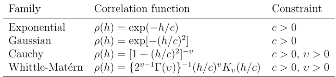
Table 3: Parametric families of correlation functions.

Family Correlation function Constraint

Exponential ρ(h) = exp(−h/c) c >0

Gaussian ρ(h) = exp[−(h/c)2_] _{c >}₀

Cauchy ρ(h) = [1 + (h/c)2]−υ c >0, υ >0

Whittle-Mat´ern ρ(h) = {2υ−1_Γ(_υ₎_}−1₍_h/c₎υ_K

υ(h/c) c >0, υ >0

parameters of the correlation function, Γ(υ) denotes the gamma function andKυdenotes

the modified Bessel function of order υ.

3.2.3

Geometric Gaussian Model

A third model we shall discuss is thegeometric Gaussian model. It is obtained by taking

Wj(x) in (3.2) as

Wj(x) = exp{λj(x)−λ2/2}, (3.8)

whereλ >0 and j(x) still follows a stationary Gaussian process with unit variance and

correlation function ρ (Davison et al., 2012). Here the bivariate marginal distribution

(53)

3.3

Inferences for Max-Stable Process Models

3.3.1

Inference based on Composite Likelihood

For the model fitting, standard likelihood method for model inference is infeasible be-cause the marginal distributions for a max-stable process are unknown for dimension three or higher. Recent works (Davison and Gholamrezaee, 2012; Padoan et al., 2010) used the composite likelihood constructed from bivariate marginal distributions (Lind-say, 1988) to jointly estimate the marginal GEV parameters and the dependence

pa-rameters. Suppose we observe the block maximum data at S sites overn blocks and let

M={Ms,t :s = 1, . . . , S;t= 1, . . . , n}, where Ms,t is the block maximum within block

t at site s. Letfijt(·;θ, β) be the bivariate marginal density of the (Mi,t, Mj,t) from the

max-stable process model specified by (3.1) and (3.2) with site i and j in block t. The

analytic form offijt is derived from the bivariate distribution for the specific model, e.g.

(3.6) in the Smith model. Let {ωij} be some reasonable choice of weight for the pair of

sites (i, j). The weighted pairwise log-likelihood of observed data is

l(β;θ;M) =

n

X

t=1

`t(β;θ;Ms,t :s= 1, . . . , S), (3.9)

where the contribution from block t is

`t(β;θ;Ms,t:s = 1, . . . , S) = S−1 X i=1 S X j=i+1

ωijlogfijt (Mi,t, Mj,t);β, θ

.

(54)

Our estimator for η> = (β>, θ>) is ˆη_n> = ( ˆβ_n>,θˆ_n>), the maximum composite likelihood

estimator of (3.9). The three MSP models discussed in Section 3.2 are viable because their bivariate marginal distributions have closed-forms and the corresponding density can be derived and used to construct pairwise likelihood, except for the Smith model, for which the trivariate marginal distributions have been derived (Genton et al., 2011). Under appropriate regularity conditions (Kent, 1982; Chandler and Bate, 2007), we

can estimate the asymptotic covariance matrix of the estimator ˆη_n> (Varin, 2008). Let

ψt(η) =∂`t/∂η, asn → ∞, ˆηnis consistent to the true parameter vectorη0, and

√

n(ˆηn−

η0)→N(0,Ω), where Ω =A−1B(A−1)> is the inverse of the Godambe information

ma-trix, with A=−limn→∞n−1Pn_t₌₁∂ψt(η)/∂η>, and B = limn→∞n−1Pn_t₌₁ψt(η)ψt>(η).

With independent replicates, we can easily estimate Ω with the sample versions of A and B. Let `t,(i,j)=ωijlogfijt (Mi,t, Mj,t);β, θ

, A can be estimated with

An =− 1 n n X t=1 ∂ψt(ˆηn)/∂η>=− 1 n n X t=1 S X i<j ∂ψt,(i,j)(ˆηn)/∂η>,

where ψt,(i,j)(η) = ∂`t,(i,j)/∂η. This matrix involves the second-order derivatives of the composite loglikelihood, which can be difficult to obtain in practice. Assuming that the bivariate marginal models are correctly specified, we can use the first-order derivatives based on the second Bartlett identity, instead of calculating the second-order derivatives

(55)

inAn. Then A can be estimated by ˆ An= 1 n n X t=1 S X i<j ψt,(i,j)(ˆηn)ψ>t,(i,j)(ˆηn).

ForB, we estimate it with

Bn= 1 n n X t=1 ψt(ˆηn)ψt>(ˆηn).

The sandwich estimator of Ω is then ˆΩn = ˆA−n1Bn( ˆA−n1)>.

3.3.2

Model Selection

Model selection can be performed based on composite likelihoods (Varin and Vidoni, 2005; Varin, 2008). A composite likelihood information criterion (CLIC) is defined as

CLIC =−2l(ˆηn)−tr[A−n1Bn] , (3.10)

which is an adaptation of the Takeuchi information criterion (TIC) (Takeuchi, 1976). The second term is a penalty on the model complexity. Models with lower CLIC are preferred.

Alternatively, the composite likelihood ratio statistic may be used. For comparing

two nested models, the ratio statistic follows a χ2 distribution asymptotically when the

(56)

distribution does not hold. Two ways have been proposed to solve this issue. Rotnitzky and Jewell (1990) proposed to adjust the asymptotic likelihood ratio statistic distribu-tion, while Chandler and Bate (2007) proposed to adjust the composite likelihood.

3.4

Extremal Coefficients

Extremal coefficient is a measure of multivariate extremal dependence for max-stable

processes proposed by Smith (1990). Consider a max-stable processZ with unit Fr´echet

margins at p locations. With the notation P ={1, . . . , p}, the extremal coefficient of a

set ofp locations {xi :i∈P} ⊂D is ζP such that

P{Z(x1)≤z, . . . , Z(xp)≤z}= exp −ζP z , z >0. (3.11)

The finite-dimensional CDF of the max-stable process belongs to the class of multi-variate extreme value distributions

P{Z(x1)≤z1, . . . , Z(xp)≤zp}= exp{−ω(z1, . . . , zp)}, (3.12)

where ω, theexponent measure function, determines the finite dimension marginal

dis-tribution, and ω is a homogeneous function of order −1:

(57)

Therefore, the extremal coefficient can be expressed via the exponent measure as

ζP =ω(1, . . . ,1). (3.13)

The extremal coefficient ζP has range [1, p], with the lower bound and upper bound

corresponding to complete dependence and complete independence, respectively. It can be interpreted as the effective number of independent sites. Properties of extremal coefficients are studied in Schlather and Tawn (2003).

Since the marginal distributions of most commonly used max-stable processes are

analytically known only for dimension 2, pairwise extremal coefficients with p = 2 are

frequently used in spatial modeling. The pariwise extremal coefficient function can

be derived from its bivariate distribution with z1 = z2 = z. For the Smith model,

ζP = 2Φ{

√

∆x0_Σ−1_∆_x/₂_}_{, which covers the whole range of possible extremal}

depen-dence. More generally, the extremal coefficients at any p sites are analytical known

for this model since its closed-form distribution function could be obtained from the

H¨usler–Reiss copula, which will be discussed in Section 5.2.2. For the Schlather model,

ζP = 1 +

q

1−ρ(||∆x||)

2 , which has a upper bound of 1 +

p

1/2 if the ρ(||∆x||) only

takes positive values. The limitation of this model is that it does not allow

inde-pendent extremes, no matter how distant the sites are; a remedy was discussed in

the work of Davison and Gholamrezaee (2012). In the geometric Gaussian model,

ζP = 2Φ{

p

(58)

max-stable process. In the realistic situation where the marginal distributions are un-known, nonparametric estimates of pairwise extremal coefficients were proposed. Smith (1990) and Schlather and Tawn (2003) proposed two different nonparametric estimates of pairwise extremal coefficients. The Schlather–Tawn method gives self-consistent es-timator in that its estimate is always between 1 and 2. Such constraint is not enforced in the Smith method. Nonparametric estimates of extremal coefficients are often used in exploratory analysis to get an idea about the spatial dependence as a function of the distance of two sites. More general forms of nonparametric estimates of extremal coefficients will be presented in Section 5.2.1.

The extremal coefficientζP could also be expressed in terms of the so-calledPickands

dependence function of the random vector (Z(x1), . . . , Z(xp)). Because the copula C

in (3.5) is of the extreme-value type, it can be expressed as

C(u1, . . . , up) = exp ( _p X j=1 loguj ! A(ς1, . . . , ςp) ) , u∈(0,1]p\ {(1, . . . ,1)}, (3.14) where ςk = loguk/ Pp

j=1loguj, k = 1, . . . , p and A : ∆p−1 → [1/p,1] is the Pickands

dependence function and ∆p−1 = {w1, . . . , wp ∈ [0,1]p−1 : w1 +· · ·+wp = 1} is the

unit simplex (see e.g. Gudendorf and Segers, 2012, for more details). Combining expres-sion (3.14) with (3.4) and equating it to (3.11), one obtains thatζP =pA(1/p, . . . ,1/p).

(59)

{xi :i∈B} with B ⊂P,|B| ≥2, can be expressed as

ζB =|B|A(wB), (3.15)

where wB is the vector of ∆p−1 such that wB,i= 1/|B| if i∈B and wB,i = 0 otherwise.

Thus, the set of extremal coefficients ζB, B ⊂ P, |B| ≥ 2, merely corresponds to the

scaled values of the Pickands dependence functionAat the pointswB,B ⊂P,|B| ≥2, of

∆p−1. As is well-known, it therefore clearly appears that the set of extremal coefficients

ζB,B ⊂P, |B| ≥2, does not fully characterize the extreme-value copulaC.

3.5

Application to Winter Maximum Daily

Precip-itation in California

3.5.1

Exploratory Analysis

In this section, we apply max-stable processes to characterizing the joint maximum daily winter precipitations observed at a network of locations in California. The data used are winter maximum daily precipitation of 192 monitoring stations in California during a 55 year period (1948–2002), which were presented as a motivating example in Section 1.2. If all 192 stations had full record of 55 years, we would have 10560 maxima, but we only have 10141 maxima — an overall missing of 3.97%. Although this missing rate seems minor, a much smaller dataset would be obtained if we only include sites with full 55

(60)

● ● ● ● ● ● ● ● ● ● ● ● ● ● ● ● ● �