WHITE MATTER
HYPERINTENSITY AND
MULTI-REGION BRAIN MRI
SEGMENTATION USING
CONVOLUTIONAL NEURAL
NETWORK
Faculty of Information Technology and Communication Sciences (ITC) Master’s thesis April 2020
Accurate segmentation of WMH (white matter hyperintensity) from the magnetic resonance image is a prerequisite for many precise medical procedures, especially for the diagnosis of vascular dementia. Brain segmentation has important re-search significance and clinical application prospects especially for early detection of Alzheimer’s disease. In order to effectively perform accurate segmentation accord-ing to the MRI characteristics of different regions of the brain, this thesis proposed an optimized 3D u-net and used WHM segmentation as a pre-experiment to select the good hyperparameters (i.e. network depth, image fusion method, and the im-plementation of loss function) to construct an image feature learning network with both long and short skip connections. Soft voting is used as the postprocessing procedure. Our model is evaluated by a 10-fold cross validation and achieved a dice score of 0.78 for binary segmentation (WMH segmentation) and accuracy of 0.96 for multi-class segmentation (139 regions brain segmentation), outperforming other methods.
Keywords: 3D Image Segmentation, Magnetic Resonance Imaging, Brain Regions, Convolutional Neural Networks.
The originality of this thesis has been checked using the Turnitin Originality Check service.
1 Introduction . . . 1
2 Related Work . . . 3
2.1 Traditional segmentation method for grayscale pictures . . . 3
2.2 Deep learning-based segmentation method for general pictures . . . . 4
2.3 Deep learning-based segmentation method for medical images . . . . 5
3 Background . . . 7
3.1 Basics of MRI . . . 7
3.2 Basics of neural networks . . . 8
3.2.1 The artificial neural networks . . . 8
3.2.2 The back propagation . . . 9
3.2.3 The activation function . . . 10
3.2.4 The loss function . . . 11
3.2.5 The optimizer . . . 13
3.3 Basics of Convolutional neural network . . . 13
3.3.1 The convolutional layer . . . 14
3.3.2 The downsampling layer . . . 16
3.3.3 The upsampling layer . . . 17
3.3.4 The normalization layer . . . 18
3.4 The ResNet and U-net . . . 19
3.4.1 The ResNet . . . 20
3.4.2 The U-net . . . 21
3.4.3 The 3D-U-Net and V-net . . . 22
4 Data . . . 24
4.1 The binary segmentation . . . 24
4.2 The multi-region segmentation . . . 25
5 Method . . . 30
5.1 Preprocessing . . . 30
5.2 Model selection and training . . . 32
5.2.1 The binary segmentation . . . 32
5.2.2 The multi-region segmentation . . . 35
5.3 Post-processing . . . 37
6 Results . . . 40
6.1 The binary segmentation . . . 40
1 Introduction
Magnetic resonance imaging (MRI) is a medical imaging technique used in radi-ology to form images of the anatomy and the physiological processes of the body (McRobbie et al. 2017). An outstanding feature of MRI imaging is that it has var-ious imaging sequences (e.g. T1, FLAIR). In T1-weighted images, there is a high signal for fat and a low signal for water, but in T2-weighted images there is a low signal for fat and a high signal for water. Faced to a variety of MRI images, the traditional method is that the physician analyzes the images through rich experi-ence and professional knowledge. However, for different physicians, and even for the same physician in different periods of time, the division and measurement of segmentations in the same image will be different, it makes manual segmentation subjective. Moreover, manual segmentation is time consuming. If physicians can evaluate the images with the help of specialized software, it will be conducive to a more accurate diagnosis and treatment of patients.
In recent years, a large number of image segmentation methods have emerged, including traditional segmentation methods and machine learning-based segmenta-tion methods. Tradisegmenta-tional segmentasegmenta-tion methods like threshold-based segmentasegmenta-tion (Kurita, Otsu, and Abdelmalek 1992) and edge detection-based segmentation (Xie and Tu 2015) are fast but sensitive to noise. Machine learning-based segmentation methods like VGGNet (Simonyan and Zisserman 2014) is highly depend on the depth of the network as well as the size and quality of training data. The fully convolu-tional network (Long, Shelhamer, and Darrell 2015) is able to do pixel-wise semantic segmentation but the results obtained are fuzzy and smooth due to upsampling, and are not sensitive to details in the image. Until now, the algorithm widely used in the field of medical image segmentation is still the u-net (Ronneberger, Fischer, and Brox 2015) proposed in 2015, and its variants.
The reason why MRI segmentation is a challenging problem is that its images have unique properties. First, MRI images are three-dimensional images and have spatial features. If the 3D image is sliced in a certain dimension and then the ordinary 2D segmentation method is applied, a lot of useful information will be lost. This thesis will prove it later in Chapter 5. Therefore, it is necessary to choose an appropriate 3D segmentation method. Another problem is the size of training data. Once the structure of the network is determined, the generalization ability depends on whether there is sufficient training set. If only one or two specific regions or lesions are needed, usually they can be labelled manually by medical experts. Furthermore, the original MRI usually has 1 channel only which means it is a gray scale image, by combining different sequences, more channels can be added. Portrait
high accuracy. These reasons make brain segmentation difficult but also meaningful. In this thesis, several experiments are performed to evaluate the performance of the existing popular networks. Based on the results of these experiments, an optimized 3D-U-net is developed in this thesis. It is applicable to extreme multiple classes segmentation and extreme small area segmentation. It uses residual units, which add the identity mapping of the input to the current convolutional layer, to enhance the learning ability of the network. The distribution of weights is considered in the design of each layer of the neural network, thereby enhancing the general-ization ability of the model. Meanwhile, to do patch merging in post-processing procedure, a new soft-vote based on probability is designed and tested as effective to increase the overall accuracy.
This thesis is structured as follows. Chapter 2 discusses briefly the general image segmentation methods, popular medical segmentation methods and their pros, cons and applications. Chapter 3 introduces the key theory behind the applied method (i.e. the basics of 2D and 3D U-net, V-net ,loss and activation functions). Chapter 4 focus on the data used in the experiments. In Chapter 5, a detailed algorithm from pre-processing to training and post-processing is explained. A comparison between the performance of the other models and the modified model introduced in this thesis is shown in Chapter 6. Chapter 7 and Chapter 8 discusses the limitations of the work and points out the potential directions of the future work and provides conclusions. The appendix contains the glossary of the thesis.
2 Related Work
In this chapter, a review of previous research works related to brain MRI segmen-tation is presented.
2.1 Traditional segmentation method for grayscale pictures
In this part, we will introduce the methods that were used to perform image seg-mentation using digital image processing, topology, and mathematics before deep learning became popular. Of course, with the increase of computing power and the continuous development of deep learning, some traditional segmentation methods can no longer be compared with deep learning-based segmentation methods, but some genius ideas are still very worthwhile for us to learn.
The simplest method is the threshold-based segmentation (Kurita, Otsu, and Abdelmalek 1992). The basic idea of the threshold method is to choose one or more gray-scale values as thresholds based on the gray-scale characteristics of the image, to compare the gray-scale value of each pixel in the image with the thresholds, and finally to segment the image according to the classes that the pixels belong to. Therefore, the selection of the thresholds influences the result a lot. The threshold method is particularly suitable for the images that the gray-scale values in different regions are significantly different. Therefore this fast method is very sensitive to noise and is not robust.
The region-based segmentation (Chang and X. Li 1994) method is a segmentation technique takes spacial information into concern. There are two basic forms of region-based extraction methods with different directions: one is region growth, which starts from one pixel and gradually merges its neighbour areas which belong to the same region to the pixel; the other starts from the whole image and gradually cuts the pixels that do not belongs to the target region. Watershed algorithm (Parvati, Rao, and Mariya Das 2008) has similarities with it. These algorithms can be seen as unsupervised or semi-supervised algorithms. This type of algorithm is ideal for segmentation of complex scenes defined by some complex objects, or for segmentation of certain natural scenes, and other similar images which lack sufficient prior knowledge.
Generally, the gray-scale value of pixels on the boundaries of different regions changes drastically. If a picture is transformed from the spatial domain to the frequency domain by Fourier transform, the edges correspond to high-frequency parts. This is a very simple edge detection algorithm and the segmentation method based on this algorithm is so called edge-based segmentation method. The
sim-deformation models (Wu and Yu 2004) have also been proposed. Edge detection cannot guarantee edge continuity and closure. Image segmentation method based on wavelet analysis and wavelet transform (J. Li 2003) can solve this problem. With the help of Hilbert transform (Dibal et al. 2018), a better result is shown.
Nowadays the most widely used traditional method in medical area is atlas-based segmentation. Atlas is a fully labeled database, for instance, the atlas of BrainWeb (Cocosco et al. 1997) contains various brain structures in CT images labeled by doctors. The earliest atlas-based segmentation was based on nonrigid registration, which registered the test image with the data in atlas, and then used the label propagation method to transfer the labels in the atlas to the test image through the registration mapping, thereby completing the segment tasks. Obviously, the atlas-based segmentation method is highly dependent on the accuracy of nonrigid registration with high computational complexity.
2.2
Deep learning-based segmentation method for general
pictures
As mentioned above, VGGNet (Simonyan and Zisserman 2014) is an example of feature encoder based segmentation method. By repeatedly stacking layers with 3 × 3 small convolution kernels and 2 × 2 maximum pooling layers, it extract image features. It builds convolutional neural network as deep as 16 to 19 layers and finds that deep networks have better performance comparing to the shallow ones. VGGNet won the runner-up of the ILSVRC 2014 competition and the champion of the positioning project. VGGNet occupies a lot of memory due to the large number of layers and the many parameters of the last three fully connected layers.
Although new models with better performance appear every year, the improve-ment to previous work is not so obvious. One of the important problems is that deep learning networks are stacked. At a certain depth, the gradient disappears, which causes the error increase effect to become worse. The gradient cannot be fed back to the previous network layer during backward propagation, which makes it difficult to update the parameters of the previous network layer and the training effect becomes worse. At this time ResNet (He et al. 2016) stood out and became an important turning point in the development process of deep learning. The core idea of ResNet
is to introduce identity mapping in the network, which directly transmitted the input information to the subsequent layers. During the learning process, only the residuals of the previous network output can be learned. The detailed algorithm of Resnet will be introduced in Chapter 3.
The convolutional neural network will lose some detailed information when sam-pling, so the purpose is to get more characteristic value. However, this process is irreversible, and sometimes the resolution of the image is too low, and details are lost during subsequent operations. Therefore, we can complete some missing information through upsampling to obtain a more accurate segmentation boundary. The most famous model in this area is the fully convolutional network (Long, Shelhamer, and Darrell 2015) so called ’FCN’. In the deconvolution-upsampling structure in FCN, the picture is first up-sampled (enlarged pixels); then convolved (weights are ob-tained through learning). FCN has become an industry benchmark in the field of image segmentation. Most of the segmentation methods will use FCN or part of it more or less.
2.3
Deep learning-based segmentation method for medical
images
DeepMedic (Kamnitsas, Ledig, et al. 2017) is a 3D multi-scale CNN with two parallel paths. The upper path extracts small area features, and then performs residual block convolution and downsampling. The lower path extracts large area features. Such a dual architecture can ensure that good detail information (local information) can be extracted in the normal resolution channel, and good high-level information (relatively large range information) can be maintained in the low resolution channel. Therefore, the segmentation information and positioning information are accurate. It is wildly used to segment brain tumors (Kamnitsas, Bai, et al. 2017).
Another method called U-net (Ronneberger, Fischer, and Brox 2015) is also widely used in the area of medical images segmentation. The original U-net is made for 2D images of cells. It is very similar to the FCN mentioned before. In the encoding part, a new scale is constructed each time it passes through a pooling layer, repeated for 5 times. The decoding part is fused at the same scale as the number of channels corresponding to the feature extraction part each time it is sampled. In this way, richer context information is obtained. In the process of decoding, detailed information is enriched through multi-scale fusion, and the accuracy of segmentation is improved. Afterwards, the same authors proposed a 3D U-net (Çiçek et al. 2016) and another group of researchers proposed the V-net (Milletari, Navab, and Ahmadi 2016) with the similar idea. They separately segmented the kidney of xenopus and the prostate volume in MRI, and achieved good results. However, only a very limited
complexity of the segmentation algorithm are issues worthy of further research. Consequently, a better multi-class (over 100 classes) segmentation method for 3D medical images is needed.
3 Background
This part of the thesis introduces some basic knowledge of medical images, neural network and image processing. These concepts will be helpful for readers to under-stand the architecture of the algorithm in Chapter 5. Three networks whose ideas are used in the algorithm in Chapter 5 are analyzed here as well.
3.1 Basics of MRI
Medical imaging has a variety of image modalities, such as MRI, computed tomog-raphy (CT), positron emission tomogtomog-raphy (PET), ultrasound imaging, and so on. Imaging can obtain images that reflect the physiological and physical characteris-tics of the human body in two and three-dimensional areas. The content of this thesis mainly focuses on the characteristics of MR imaging. Each element in the two-dimensional image is called a pixel, and each element in the three-dimensional area is called a voxel. In some cases, the three-dimensional image can be repre-sented as a series of two-dimensional slices for observation. The advantage is that the calculation complexity is low and requires less memory.
Magnetic resonance imaging (MRI) is the most widely used technique in the field of radiography. As a dynamic and flexible technology, MRI can achieve vari-able image contrast. This process is achieved by using different pulse sequences and changing imaging parameters corresponding to the longitudinal relaxation time (T1) and lateral relaxation time (T2). T1 and T2-weighted imaging signal strength is related to the characteristics of specific tissues (Shenton et al. 2001). Imaging parameters used in the dataset of this thesis is listed as Table 3.1. The 3D images used in this study are rebuilt from a number of 2D slices in the axial direction.
Table 3.1 Imaging parameters of the dataset.
Parameters FLAIR T1 Echo time 100-140 ms 4-7 ms Repetition time 6000-10000 ms 10-25 ms Inversion time 2000-2400 ms Flip angle 15◦−30◦ Voxel size 0.4−1×0.4−1×5−7.5mm3 0.5−1×0.5−1×1−1.5mm3 Number of slices 15-38 256
MRI has a good imaging ability for soft tissues, very high resolution, and a high signal-to-noise ratio. Different pulse sequences can be used to obtain multi-channel images with varying contrasts, which can be used for target segmentation and classification of different anatomical structures (Vandenberghe and Marsden
3.2 Basics of neural networks
Before we talk more about neural networks, let us understand some terms. Strictly speaking, the neural network to be created is called an artificial neural network (ANN), to distinguish it from the real neural network in the human brain (a network of brain cells connected). We may also see neural networks to appear under some names, such as connected machines (also known as connectionism in this field), parallel decentralized processors (PDP), thinking machines, etc., but we will use the term ”neural network”. It is used to refer to ”artificial neural networks”.
3.2.1
The artificial neural networks
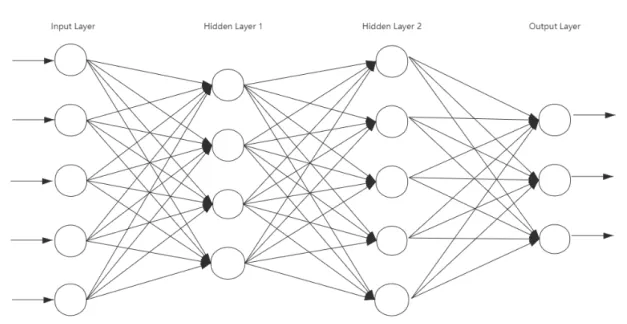
A typical neural network consists of several, hundreds, or thousands of artificial neurons called ”units”. They are arranged in a series of layers, and each layer is connected to each other. Some of these neurons are called ”input units” and are used to receive a variety of information from the outside world. Neural networks use this information to learn, recognize patterns, or perform other processing. There are also some neurons on the other side of the neural network, which are opposite to the ”input unit”. They show the learning status of the neural network. These neurons are called ”output units”. Between the ”input unit” and the ”output” unit there are also one or more layers composed of ”hidden units”, which together with the ”input layer” and ”output layer” form a neural network. Figure 3.1 presents an example of a four-layer simple fully connected neural network.
Fully connected means that for all the layers that is not the input layer, each neuron inside is connected to all the neurons in the preceding layer. The connection is the ”weight”, which can be positive (when one unit fires another) or negative (when one unit suppresses another). The higher the weight value, the greater the influence of one unit on the other unit (this is the same principle that human brain cells stimulate each other through synapses). Figure 3.2 contains an example of a perceptron in the ith hidden layer. Activation computation of one neuron is repre-sented mathematically as:
y=f(
n ∑
j=1
Figure 3.1 An example of neural network with an input layer, 2 hidden layers and an output layer.
Figure 3.2 An example of a perceptron of theith layer.
where y is the output of this neuron, f(x) is the activation function and bi is the
bias. Bias can help to improve the flexibility of neural networks. wij is the weight
between the neuron before and the current neuron.
3.2.2 The back propagation
Information is moved through neural networks in two ways, forward and backward. When the neural network is in training period or predicting period, the information
the unit connected to it.
The neural network learns using a feedback mechanism called ”back propagation” (Werbos 1974), which consists of both the forward propagation process and the back propagation process. In the forward propagation process, if the final output is different from the optimal value, then the sum of the square of the difference is computed and transfer to back propagation, and the partial derivative of the objective function on the weight of each neuron is found layer by layer to form the target. The ladder of the function’s weight vector is used as the basis for modifying the weight. The learning of the neural network is completed in the process of modifying the weight. When the error (the sum of the square of the difference) reaches the expected small enough value, the process ends.
3.2.3
The activation function
In neural networks, there is a functional relationship between the inputs and outputs of the hidden and output layer nodes. This function is the activation function. If there is no activation function, the input and output have a linear relationship, but in reality many models are non-linear. The introduction of the activation function can increase the non-linearity of the model. The activation functions used in the network in Chapter 5 are ReLU (Bishop et al. 1995), sigmoid (Cybenko 1989) and softmax (Bishop et al. 1995).
Sigmoid function is also called Logistic function, which has a very important position in the field of machine learning. First, Sigmoid’s equation is
Sigmoid(x) = 1
1 +e−x. (3.2)
Its domain is (∞,+∞) and range is (0,1). The function is continuous and smooth in the domain and has derivative everywhere (Cybenko 1989). In most cases, there is no way to know the form of the probability distribution of unknown events, and when it is not known, the normal distribution is the best choice because it is the most likely form of expression of all probability distributions. After assuming that the probability distribution of an event conforms to the law of normal distribution, to analyze its possible probability, it depends on its integral form. The format of the integral of the Sigmoid function is very similar to the normal distribution
function. Because of the simple equation and very small calculation of Sigmoid, it is selected as a substitute function. Sigmoid functions are generally used to solve binary classification problems.
When the Sigmoid function is used as the activation function and the gradient is less than 1 in the deep model, the learning ability will be attenuated layer by layer. This phenomenon is particularly obvious and will cause the model to stagnate called vanishing gradient problem (Hochreiter et al. 2001). For non-linear functions, rectified linear unit (ReLU) has no gradient disappearance problem because the gradient of the non-negative interval is constant. The equation of ReLU is shown below,
ReLU(x) = max(0, x). (3.3) For linear functions, ReLU is more expressive, especially in deep networks. The model implemented by ReLU can better mine related features and fit the training data. In deep learning, we generally use ReLU as the activation function of interme-diate hidden neurons. In AlexNet (Krizhevsky, Sutskever, and G. E. Hinton 2012) it is proposed that using ReLU to replace the traditional activation function is a major advance in deep learning.
Softmax (Bishop et al. 1995) is used in the multi-classification process. It maps the output of multiple neurons into the (0,1) interval with the function
Sof tmax(x)i =
exp(xi) ∑
jexp(xj))
. (3.4)
Suppose we have an array, xi representing the i-th element in the array. Then
the Softmax value of this element is the exponent of the element, divided by the sum of the exponents of all elements.
3.2.4
The loss function
In the calculation of neural networks, we often need to calculate the difference between the score S1 calculated according to the feed forward propagation of the
neural network and the score S2 calculated according to the correct labeling, and
to calculate loss before applying back propagation. Loss is usually defined as cross entropy. The loss function guides the direction of model optimization.
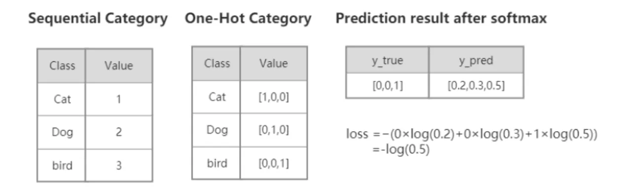
It is very easy to calculate the cross entropy loss through out the softmax value. Cross entropy measures the difference between the true sample label and the pre-dicted probability. For binary classification problem, the loss function called binary cross entropy is applied. For multiple classification problem, the categorical cross entropy is applied. Equation 3.5 shows the basic form of cross entropy for an array
to one-hot vector before training. One hot coding is the process of transforming categorical variables into a form that machine learning algorithms can easily use. It uses the bit status register to encode each state. Each state has only one bit that is valid and all the other bits are 0. Figure 3.3 is an example of how to change normal sequential label to one hot label and calculate the cross entropy.
Figure 3.3An example of one-hot coding a 3-class case. Including the one-hot embedding and loss calculation
The dice loss is proposed in V-net (Milletari, Navab, and Ahmadi 2016). One of the reasons is that the anatomical structure of interest only occupies a very small area of the scan, so that the learning process falls into the local minimum of the loss function. Therefore, we must increase the weight of the prospects. Dice can be understood as the degree of similarity between the two contour areas, which is defined as:
Dice_score(A, B) = 2× |A∩B|
|A∪B| , (3.6)
where A and B are used to represent the point set contained in the two contour areas.
Dice can also be expressed as:
Dice_score= 2×T P
2×T P +F P +F N, (3.7)
false negatives, respectively. To prevent the denominator from being zero, a Laplace smoother can be added to the dice score:
Dice_score= 2×T P + 1
2×T P +F P +F N + 1. (3.8)
The dice loss is the opposite to dice score. Here we use1−dicescoreto represent dice loss:
Dice_loss= 1− 2×T P + 1
2×T P +F P +F N + 1. (3.9)
3.2.5 The optimizer
Deep learning can be reduced to an optimization problem, which minimizes the objective functionJ(θ); in the optimization process, first the gradient∇J(θ)of the objective function is solved and then the parameter θ is updated to the negative gradient direction,θt =θt−1−η∇J(θ)where η is the learning rate, which indicates
the step size of the gradient update. The algorithm that the optimization process depends on is called an optimizer. It can be seen that the two cores of the deep learning optimizer are the gradient and the learning rate. The former determines the direction of parameter update and the latter determines the degree of parameter update. The reason why the deep learning optimizer uses gradients is that for higher-dimensional functions, the higher-order derivative has a large computational complexity and is not practical for the optimization of deep learning. There are many types of deep learning optimizers, and research in the academic world has also been very active. Adam (Kingma and Ba 2014) is mainly used in the network proposed in this thesis.
Adam combines the advantages of two optimization algorithms, AdaGrad (Duchi, Hazan, and Singer 2011) and RMSProp (Tieleman and G. Hinton 2012). Adam is simple to implement, computationally efficient, and requires less memory comparing to AdaGrad and RMSProp. It is very suitable for large-scale data and parameter scenarios.
3.3
Basics of Convolutional neural network
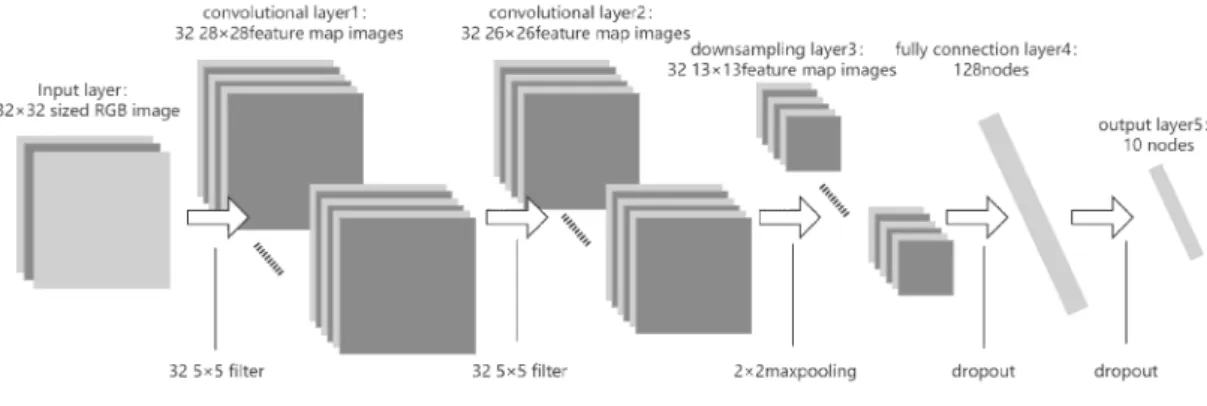
Convolutional neural network (Bouvrie 2006) makes the image go through a series of convolutional layers, non-linear layers, pooling (downsampling) layers and fully connected layers, and finally get the output. Figure 3.4 represents an example of a 2D CNN with 2 convolutional layers, a maxpooling layer and 2 fully connected layers. The output can be the probability of an individual classification or a group of classifications that best describe the image content. The challenge is understanding how each of these layers works.
Figure 3.4 A 2D CNN example. The input is a 32×32 3-channel RGB image.
3.3.1 The convolutional layer
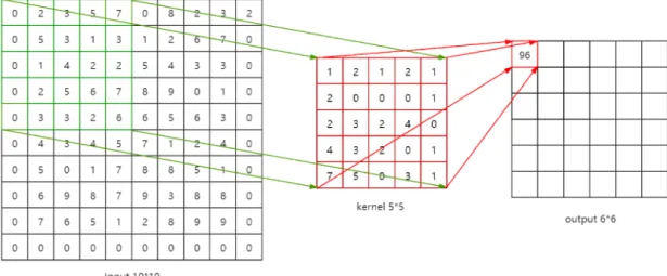
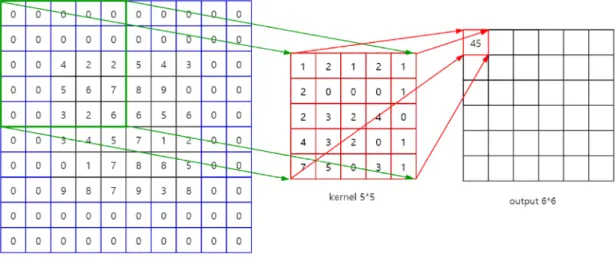
The first layer of a CNN is usually a convolutional layer. As the example shown in Figure 3.4 ,the input is an array of 32×32×3 pixel values. Imagine that there is a 5×5 sized frame on the upper left corner of the image. In machine learning terms, this frame is called a filter (kernel), and the area inside the frame is called a receptive field. The depth of the filter must be the same as the depth of the input (to ensure that mathematical operations can be performed), under gray-scale condition the depth is 1 and under RGB condition the depth is 3, so the filter size is5×5×3. The frame can slide on the image freely and on each position it can do a convolution operation, that is, the value in the filter is multiplied(dot product) by the original pixel value in the image. The sum (sum of 75 products in this case) indicates the convolution result of the current position of the frame. The process is repeated at every position on the input. (The next step is to move the filter 1 unit to the right, then 1 unit to the right, and so on.) Each specific position on the input produces a number. After the filter slides through all the positions, we will get an array of 28 x 28 x 1, which we call activation map or feature map. The reason for a28×28array is that a5×5filter can cover 784 different positions on a32×32input image. These 784 positions can be mapped into a 28 x 28 array. Figure 3.5 shows an example of a10×10sized images and a 5×5 sized filter. Note that there is only one kernel in this example and if there are 3 kernels the output would change to 36×6matrices. The more filters used, the better the spatial dimensions are preserved.
For two-dimensional convolution, the convolution kernel performs sliding window operations on the spatial dimensions of the input image (that is, (height, width) two dimensions). Each group of values in the sliding window are convolved to the value of a pixel (or a voxel in 3D cases) in the output image. The difference in Figure 3.6 between 3D and 2D convolution is that the input image has one more depth dimension and the convolution kernel has one more dimension, so the convolution
Figure 3.5An 2D convolutional layer example. The input is a10×101-channel grayscale image.
kernel performs sliding window operation on the spatial dimensions (height and width) and depth dimensions of the input 3D image. Each sliding window performs related operations with the values in the window to obtain a value in the output 3D image (see Figure 3.6(b)).
(a) 2D example. (b) 3D example.
Figure 3.6 One channel case for both 2D and 3D convolution.
To change the behavior of the convolutional layer, there are two main parameters that we can adjust. Padding and stride can influence the convolutional layer by changing the number of steps that the filter moves which will lead to different results. The stride influences the number of convolution operations. In the previous example, the filter convolved the input by moving one unit at a time. The stride is the number of pixels or voxels that the filter moves at a time. In that example, the stride is set to 1 by default. The stride is usually set to ensure that the output is an integer and not a fraction. Figure 3.7 shows a7×7input image and a 3×3filter (without considering the third dimension for simplicity) with strides of 1 and 2.
In the Figure 3.5, it is easily found that the output has a different size comparing to the input. The size of the image is shrinking rapidly dur to the information loss happened at the boarder area. In the early layers of the network, we wanted to
(a) The stride is 1. (b) The stride is 2.
Figure 3.7 An example of different strides for a 7×7 input and a 3×3 kernel, the outputs are different with different strides.
retain as much information as possible about the original input so that we could extract those low-level features. By adding zero padding of sized 2 with the same filter and stride, the size of the output can be kept as10×10. Figure 3.8 shows an example that the output remains the same size as the input.
Figure 3.8 A zero-padding example. The input is a6×6 1-channel grayscale image and the output remains the same size.
3.3.2
The downsampling layer
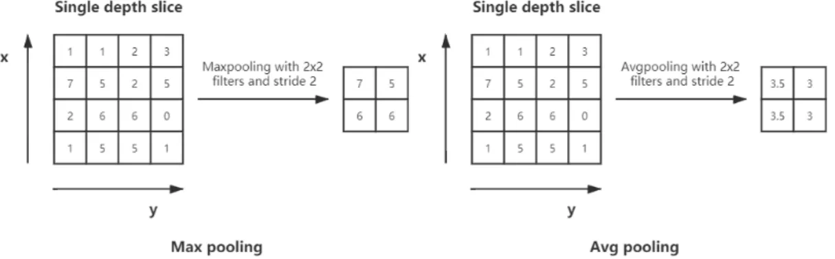
In Figure 3.4 there is a downsampling layer. There are also several methods to choose from in this category, the most popular of which is max-pooling. It basically uses a filter (usually 2x2) and a stride of the same length. The input image is divided in to several sub-regions and the size of each sub-region is equals to the size of the filter. Each value of a pixel or voxel in the output is the maximum
value in a sub-region. There are other options for the pooling layer, such as average pooling (M. Lin, Q. Chen, and S. Yan 2013) (see Figure 3.9) and L2-norm pooling (Carreira et al. 2012). The intuitive reasoning behind this layer is that once we know a particular feature in the original input (which will have a high activation value here), its relative position to other features is more important than its absolute position. It is conceivable that this layer greatly reduces the spatial dimension of the input volume (the length and width have changed, but the depth has not changed). This serves two main purposes. The first is that the number of weight parameters is reduced, thus reducing the computational cost. The second is that it can control overfitting. Overfitting refers to a model that matches the training sample so much that it does not produce good results when used in validation and testing groups.
Figure 3.9 Two downsampling examples. The left one is the max-pooling and the right one is the average-pooling.
In Figure 3.4 there are also two dropout layers. The dropout layer (Srivastava et al. 2014) will ”drop out” a random activation parameter set in this layer, that is, set these activation parameter sets to 0 in the forward pass. In a way, this mechanism forces the network to become more redundant. What this means is that the network will be able to provide a suitable classification or output for a particular sample, even if some activation parameters are discarded. This mechanism will ensure that the neural network will not ”over-match” the training samples, which will help to alleviate the problem of overfitting.
3.3.3
The upsampling layer
In the field of deep learning applied in computer vision, the size of the output tends to become smaller after the features of the input image are extracted by a convolutional neural network (CNN), and sometimes we need to restore the image to its original size for further calculations (e.g. semantic segmentation of images).
complete inverse process of forward convolution. Deconvolution is a special type of forward convolution. First, it expands the input by adding 0 according to a certain proportion, then rotates the convolution kernel, and finally performs the forward convolution. The following Figure 3.10 depicts an example of a deconvolution process.
Figure 3.10 The image size changes from3×3 to5×5 after deconvolution.
3.3.4
The normalization layer
When passing the images to the neural network, the images should be normal-ized beforehand. Normalization is to transform the original image to be processed into a corresponding unique standard form through a series of transformations (the standard form image has invariant characteristics for affine transformations such as translation, rotation, and scaling). That is, the invariant moment of the image is used to find a set of parameters so that it can eliminate the impact of other trans-formation functions on the image transtrans-formation. Normalization accelerates the speed of gradient descent to find the optimal solution. The most common method is the zero-mean normalization. The processed data conforms to the standard normal distribution, that is, the mean is 0, the standard deviation is 1, and its conversion function is
f(x) = x−µ
σ , (3.10)
where µ is the mean of all pixels (voxels) and σ is the standard deviation of all data.
The method used in this thesis is the Min-max normalization. This algorithm is a linear transformation of the original data so that the result falls into the interval [0,1]. The conversion function is as follows:
f(x) = x−min(X)
max(X)−min(X), (3.11)
where min(X) is the minimum value of all pixels (voxels) and max(X) is the maximum.
Normalization happens not only before the network, but also along the network. As the training progresses, the parameters in the network are continuously updated with gradient descent. On the one hand, when the parameters in the underlying network change slightly, these weak changes are amplified as the number of network layers deepens due to the linear transformation and non-linear activation mapping in each layer (similar to the butterfly effect). The change of parameters causes the input distribution of each layer to change, and the upper-layer network needs to constantly adapt to these distribution changes, making our model training difficult. This phenomenon is called Internal Covariate Shift (Ioffe and Szegedy 2015). Be-cause of the internal covariate shift the network needs to be constantly adjusted to adapt to changes in the input data distribution, resulting in a decrease in the network learning speed. Meanwhile, the network training process is easy to fall into the gradient saturation region, which slows down the network convergence speed.
For each hidden layer neuron, the input distribution that gradually maps to the non-linear function and moves closer to the limit saturation zone of the value interval is forced to return to a relatively standard normal distribution with a mean of 0 and a variance of 1, so that the input value of the non-linear transformation function is in a more sensitive area to avoid the problem of gradient disappearance. This is the idea of batch normalization (Ioffe and Szegedy 2015).
3.4
The ResNet and U-net
The network designed in this thesis contains the main idea of the ResNet and the U-net. The networks and their variants are briefly introduced in this section.
or explosion, there is also the problem of degradation of deep networks which refers to the phenomenon that deep neural network is sensitive to the small changes and make it very difficult to converge (Duvenaud et al. 2014).
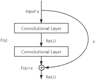
Kaiming He (He et al. 2016) proposed residual learning to solve the degradation problem. For a stacked layer structure (stacked by several layers), when the input is x, its learned features are recorded as H(x). Now we hope that it can learn the residualF(x) =H(x)−x. In fact, the original learning characteristics are F(x) +x. For example, in the division of 13 by 5 we have13 = 2×5 + 3, 3 is the remainder. The 2×5 can be seen as the learned feature, 13 is the input and 2×5−13 = −3
is the residual. However, in the division of 13 by 5 and 14 by 5 gives the same quotient(learned feature), the way that they differ from each other is the different residuals. Residual learning is easier than direct learning of original features. The structure of residual learning is shown in Figure 3.11. This is similar to a ”short circuit” in a circuit, so it is called a short-cut connection.
3.4.2
The U-net
U-Net (Ronneberger, Fischer, and Brox 2015) is one of the earliest algorithms for se-mantic segmentation using fully convolutional networks. The symmetric U-shaped structure containing compression paths and expansion paths was very innovative at the time and affected some of the later designs of the networks for image segmen-tation. The name of the network is also derived from its U-shape.
U-Net’s U-shaped structure is shown in Figure 3.12. The network is a classic fully convolutional network (that is, there is no fully connected operation in the network). The input of the network is an572×572 input image tile with a mirror operation on the edges. The left side of the network (red line) is a series of down-sampling operations consisting of convolution and max-pooling. This part is called contracting path. The compression path is composed of 4 blocks. Each block uses 3 effective convolutions and 1 Max Pooling downsampling. After each downsampling, the number of feature maps is multiplied by 2, so we have the feature map size changed as shown in the figure. The result is a feature map with the size32×32.
Figure 3.12 The architecture of the U-net1.
The right part of the network (green line) is called the expansion path in the paper. It also consists of 4 blocks. Before the start of each block, the size of the
the extended path still uses the effective convolution operation, and the size of the resulting feature map is388×388. Since this task is a binary classification task, the network has two output feature maps. Valid padding increases the difficulty and universality of model design, so U-Net uses a loss function with boundary weights. This thesis will not go into details here.
The merge operation in the U-net is to concatenate two matrices in the last dimension. It can be seen as a long skip connection. The merge operation in the ResNet is a simple add operation, it adds the corresponding elements in two matrices. It can be seen as a short skip connection. It is proved that both short and long skip connections (Drozdzal et al. 2016) are important in biomedical image segmentation.
3.4.3
The 3D-U-Net and V-net
3D U-Net (Çiçek et al. 2016) is based on the previous U-Net structure. The dif-ference is that all 2D operations are changed to 3D operations. At the same time, batch normalization is used in order to speed up convergence and avoid training bottlenecks. During training, it is normalized and standardized according to the current batch information. At the same time, compared with U-Net, a weighted softmax loss function is used, and the weight of unlabeled pixels is set to zero, and only the labeled pixels can be learned. The weight in the softmax loss expression of the background is reduced, and the weight of the foreground is increased.
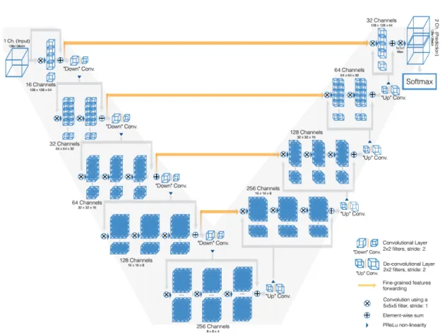
The entire network of V-net (Milletari, Navab, and Ahmadi 2016) is divided into compression paths and uncompression paths, that is, feature maps are reduced and expanded as Figure 3.13. Each stage reduces features by half, and residual learning is added to each stage to accelerate convergence.
The circle and cross in Figure 3.13 represent a convolution with a convolution kernel of 5×5×5 and a stride of 1. It can be seen that padding 2×2×2 can keep the feature size unchanged. At the end of each stage, a convolution kernel of 2×2×2 and a stride of 2 are used. The feature size is reduced by half (the advantage is that there is no need to save pooling switches, so the smaller memory footprint). The entire network uses the PReLU (He et al. 2015) nonlinear unit. A
1×1×1 convolution is added to the end of the network,the data is processed as the same size as the input and finally a softmax function is applied.
Figure 3.13 The architecture of the V-net (Milletari, Navab, and Ahmadi 2016).
The network learns the idea of U-Net, and sends the underlying features of the reduced end to the corresponding positions of the enlarged end to help reconstruct high-quality images and accelerate model convergence. It uses the dice loss instead of the loss used by the U-net. The 3D-U-Net and V-Net shows two different directions of development in 3D image processing. The U-Net kept the original architecture and optimized the distribution in each layer as well as the training method. While the V-Net changed the architecture by adding to new components (residual units).
is used to do multi-class segmentation.
4.1 The binary segmentation
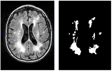
The dataset is a part of the Leukoaraiosis And DISability (LADIS) Study (Waldemar 2002). The study followed patients for three years and took their MRI images (T1-, T2-(T1-, proton density-weighted and FLAIR (Fluid-Attenuated Inversion Recovery) pulse sequences) as well as their physical indicators. In this thesis, FLAIR images from 606 patients and the images of manually segmented white matter hyperintensity area are used. Below there are two examples of a slice of the images.
(a) FLAIR image example. (b) White Matter Hyperintensity example.
Figure 4.1 An example of the FLAIR image and the manual segmentation of white matter hyper-intensities from the corresponding axial slice.
The Figure 4.1(a) is an axial slice of the FLAIR image. The original FLAIR images contain not only the brain tissues but also the brain areas. The non-brain areas do not contribute to the non-brain segmentation. They are irrelevant features or noise features, Especially in T1 images, the intensity of eyes is similar to some brain tissues. The non-brain areas will extend the total training time, decrease the model accuracy and increase the risk of overfit. A brain mask (Lötjönen, Robin
Wolz, Koikkalainen, Julkunen, et al. 2011) can be generated by atlas-based method from T1 images. It is a 3D image with values 0 and 1 only. Value 0 stands for non-brain area and value 1 stands for non-brain area. Use the non-brain mask on all the FLAIR images and T1 images, this process is called skull-stripping. Originally, the thickness of one FLAIR slice is about 6mm. Processed so that all the images are spatial normalization to same space with 1 mm isotropic space with size of180×256×256
and values are z-score normalized with zero mean and standard deviation equals to 1. The manually labeled images have the same size as the FLAIR images. In the manually segmented images, all the WMH areas are labeled as 1 and the background is labeled as 0. Table 4.1 compared the two images after pre-processing.
Table 4.1 Binary segmentation training data and testing data.
FLAIR images label images
quantity 606 606
size 180*256*256*1 180*256*256*1
value range mean=0, std=1 {0,1}
type gray-scale gray-scale
use training data ground truth
feature WMH is brighter than normal white matter
label 0 is the background label 1 is the WMH
4.2
The multi-region segmentation
It is extremely time consuming to generate large number of training samples with different brain regions segmented manually. Consequently, an alternative approach was selected in this thesis. A dataset of 1151 MRI images is generated by utilized an atlas-based segmentation method (Lötjönen, Robin Wolz, Koikkalainen, Thurfjell, et al. 2010). This method segments automatically the T1 images into 139 brain regions. The T1-weighted images were used as training set and the automatic seg-mentations as the ground truth. Figure 4.2 shows a T1 image from a patient and its segmentation. Different colors in Figure 4.2(b) stand for different brain regions. The automatically generated dataset contains segmentation errors. In order to test the performance of the network on manually segmented data, we prepared 80 T1-weighted images and the manually labeled results made by medical experts.
In addition to producing accurate segmentation, it is important that the au-tomatically generated segmentations are consistent. Therefore, a dataset from 20 patients that had two T1 images acquired during the same time was used. Also, the manual segmentations were available for both images. The difference between the results from one person shows the consistency of the model. The two sets of slices in Figure 4.3 are nearly the same except some system errors and random errors.
(a) T1 image example. (b) Segmentation from atlas-based seg-mentation.
Figure 4.2 An example of T1 image and its atlas-based segmentation result.
Figure 4.3 The two T1 images from one patient from the consistency dataset.
A brief summary of the data used in the multi-region segmentation is listed in the Table 4.2.
In the ground truth from both manual data (data segmented by expert) and automatic data (data segmented by atlas-based method) the value range is a set of 140 values from 0 to 139. Index 0 stands for the background and all the rest 139 numbers are the indexes of brain regions. Most brain regions appear both in the left brain and the right brain, so the area on the left and right is marked with two indexes separately. Some regions like cerebellum are located in the middle of the brain, so only one index is given to the region like this. The Table 4.3 shows the position and index of each region.
Table 4.2 The summary of the three datasets. Atlas-based segmentation dataset Manual segmentation dataset Consistency dataset quantity (T1, GT) 1151 ,1151 80, 80 40, 40 size 180*256*256*1 180*256*256*1 180*256*256*1 value range (T1, GT) [0,1], {0,1...139} [0,1], {0,1...139} [0,1], {0,1...139}
type gray-scale gray-scale gray-scale
use training and validating training and validating consistency testing source the GT is generated
by atlas-based method the ground truth is manually labeled feature
In the ground truth, the area with label 0 is the background and label 1-139 are different brain regions.
the two images from one patient should have the same result
Table 4.3 The indexes, positions, and names of the 139 brain regions.
position name left right
Ventricles
3rd ventricle 1 4th ventricle 2 5th ventricle 3 Inferior lateral ventricle 23 22
Lateral ventricle 25 24
Deep gray matter
Accumbens area 5 4 Caudate 10 9 Pallidum 27 26 Putamen 29 28 Thalamus proper 31 30 Temporal Lobe Amygdala 7 6 Hippocampus 21 20 Entorhinal area 57 56 Fusiform gyrus 63 62 Inferior temporal gyrus 69 68 Middle temporal gyrus 91 90 Parahippocampal gyrus 105 104
Planum polare 115 114 Planum temporale 119 118 Superior temporal gyrus 133 132 Temporal pole 135 134 Transverse temporal gyrus 139 138
Vessel 35 34 Optic chiasm 36
Occipital Lobe
Calcarine cortex 51 50 Cuneus 55 54 Inferior occipital gyrus 67 66 Lingual gyrus 71 70 Middle occipital gyrus 81 80 Occipital pole 93 92 Occipital fusiform gyrus 95 94 Superior occipital gyrus 129 128
Cerebellum
Cerebellum exterior 12 11 Cerebellum white matter 14 13 Cerebellar vermal lobules I-V 37 Cerebellar vermal lobules VI-VII 38 Cerebellar vermal lobules VIII-X 39
Frontal Lobe
Basal forebrain 41 40 Anterior cingulate gyrus 43 42 Anterior insula 45 44 Anterior orbital gyrus 47 46 Central operculum 53 52 Frontal operculum 59 58 Frontal pole 61 60 Gyrus rectus 65 64 Lateral orbital gyrus 73 72 Middle cingulate gyrus 75 74 Medial frontal cortex 77 76 Middle frontal gyrus 79 78 Medial orbital gyrus 83 82 Precentral gyrus medial segment 87 86 Superior frontal gyrus medial segment 89 88 Opercular part of the inferior frontal gyrus 97 96 Orbital part of the inferior frontal gyrus 99 98 Posterior orbital gyrus 113 112
Precentral gyrus 117 116 Subcallosal area 121 120 Superior frontal gyrus 123 122 Supplementary motor cortex 125 124 Triangular part of the inferior frontal gyrus 137 136
Parietal Lobe
Angular gyrus 49 48 Postcentral gyrus medial segment 85 84 Posterior cingulate gyrus 101 100
Precuneus 103 102 Posterior insula 107 106 Parietal operculum 109 108 Postcentral gyrus 111 110 Supramarginal gyrus 127 126 Superior parietal Lobule 131 130
segmentation on different types of datasets are proposed.
5.1 Preprocessing
The preprocessing procedures for FLAIR images and T1 images are slightly different. The work flows are listed in the Figure 5.1 below.
(a) Preprocessing of FLAIR. (b) Preprocessing of T1. Figure 5.1 Preprocessing work flows.
Factors such as the patient location in the scanner, the scanner itself, and many unknown issues can cause differences in brightness on the MR image. In other words, the intensity value (from black to white) can vary within the same tissue. This is called a bias field. Bias fields cause non-uniformities in the magnetic field of the MRI machine. If the offset field is not corrected, all imaging processing algorithms will output incorrect results. Before segmentation or classification, a pre-processing
step is required to correct the effect of the bias field. An N4 bias field correction tool(Avants, Tustison, and Song 2009) is applied to all the images.
The min-max normalization method (Equation 3.11) is applied to the FLAIR images. Hence, all the values in images are in interval [0,1]. No need to normalize the values in T1 images because they falls in the [0,1] interval naturally. For the label images of T1 images, The label is changed to one-hot vectors, so the dimension is changed from180×256×256×1to180×256×256×140. The last dimension of the ground truth images indicates the class that a voxel belongs to. In the matrix, only voxels that belong to class i are labeled as 1 and 0 otherwise. Class 0 is the background and classes 1, 2, ... 139 are different brain regions shown in Table 4.3. Class imbalance of data is often encountered in machine learning, also known as class skew. It also happened in the images used in this thesis. For instance, in binary segmentation, the number of voxels of WMH is 20000 in average. The total number of voxels in a FLAIR images is over107. If the system predicts all the voxels as background, that is it wrong predicts all the true cases, the accuracy is still over 99%. Therefore, it is meaningless to measure a model with its accuracy. The most straightforward method to solve the imbalance problem is to make the data balanced. The border containing background only is discarded. Then the size of the image shrinks to160×192×160. The data is more balanced than before but it is still far from half to half.
During the CNN learning and training process, instead of processing an entire image at a time, the image is first divided into multiple small blocks. The kernel (or filter or feature detector) only views one block of the image at a time. The small block is called a patch, and the filter is moved to another patch of the image, and so on. The CNN kernel(filter) processes only one patch at a time, not the entire image. This is because we want the filter to process small patches of the image in order to detect features (edges, etc.) within the GPU memory limitation. This also has a good regularization property, because the number of parameters we estimate is small, and these parameters must be ”good” in many areas of each image (Z. Yan et al. 2017).
For a simple CNN, the size of the patch that minimizes information loss is the size of the receptive field. The receptive field (Dumoulin and Visin 2016) can be briefly defined as the region in the input space that a particular CNN’s feature is looking at. For a 2D convolutional layer with a3×3filter, each pixel in the output corresponds to a 3×3area in the input. Thus, the receptive field is 3×3. In spite of this fact, as the size of the receptive field increases with the number of neural network layers, the size of the receptive field is close to the size of the whole image. Under these circumstances, the size of a patch has to be smaller than the receptive field with some information loss.
window slides a length of 32 units, it generates a smaller cube that has the same size as the window.
Figure 5.2 The MRI image with three patches generated.
It is easy to count that from each 160×192 ×160 sized image, a number of
4×5× 4 = 80 patches can be produced. Over-sampling can help to make the data more balanced. There are other 20 patches randomly generated from the inner area of the image which is labeled red in Figure 5.3. The size of the inner area is
96×128×96. The WMH is more likely to appear in this area, so the proportion of true cases is higher than in the whole image.
5.2
Model selection and training
5.2.1 The binary segmentation
A 3D image can be seen either as a simple 3D image or as a set of 2D images. For instance, a 3D image with the size of 160×192×160 can be seen as 160192×160
Figure 5.3 The red area shows the region from where the random patched are generated.
Figure 5.4 The 3D to 2D process.
As the inputs are 2D images rather than 3D images, the network contains 2D convolution layers and 2D deconvolution layers only. It saves training time, simplifies the computation and reduces the memory usage. To compare the performance of 2D inputs and 3D inputs, a simple encoder and decoder network without patching is built.
Note that when the 3D image is transformed to a group of 2D images, the 2D images in a group are ordered. So as to let the network learn about the sequential information, the images in the group should not be shuffled and the size of the batch should be set as the quantity of the images from one 3D image. This sacrifices some generalization performance of the model, but learns more information from each group of images.
The model as simple as the one in Figure 5.5 is not sufficient to learn all the features, but a deeper network is needed. With the inspire of the net, a 3D
U-(a) One-layer network with 2D input.
(b) One-layer network with 3D input. Figure 5.5 The one-layer models.
net with long connection only and batch normalization but still without patching is created (Figure 5.6).
The network in Figure 5.6 has four compressing layers and four decompressing layers. In each compressing layer, the convolution is done twice with batch normal-ization and activation. Two compressing layers are connected with a max-pooling operation. After the max-pooling, the length, width and depth in each feature map are halved. In each decompressing layer, a transposed convolutional layer doubles the length, width and depth in each feature map but halves the quantity of feature maps. Then the feature maps are concatenated to the feature maps with the same dimensions that were generated from the compressing layers. Afterwards, the above steps (two convolutional layers) in the compressing layers are repeated in decom-pressing layers. Finally, Sigmoid activation method is used to give the output.
Instead of using long skip connection only, merging the network in Figure 5.6 with the short cut in Figure 3.11 will give a different network shown in Figure 5.7(a) and Figure 5.7(b). Giving different inputs (use patching or not) the necessary of patching can be tested.
In the networks shown in Figure 5.7(a) and Figure 5.7(b), the only difference is the size of each feature map. They contain four compressing layers and four
Figure 5.6 The basic 3D U-net with no patching.
decompressing layers as well but the operations in each layers are different from the layers in Figure 5.6. In the first three compressing layers, there are two convolutional layers with kernels size of3×3and 1×1that are used to extract the features from the image. Then we normalize both results and sum the two results together. The result from3×3 kernel is the learned feature and the result from 1×1 kernel can be seen as the residual. The sum of two results is activated by ReLU and passed to the next layer. In the last compressing layer and the first three decompressing layers, after the two results from kernels size of3×3and 1×1 are added together and activated. Finally a dropout layer with the dropping rate of 0.5 is added at the end. While in the last decompressing layer there is no dropout layer, the operation is the same as the first four compressing layers, except the1×1convolutional layer with a Sigmoid activation layer to get the output.
5.2.2
The multi-region segmentation
There are only two classes in the binary segmentation and the two classes are labeled as categorical (0 and 1) by default. Conversely, the labels are numerical in the multi-region segmentation. After changing the labels to one-hot labels, the dimension of the ground truth is changed from160×192×160×1to160×192×160×140. Such a big matrix is not suitable to be passed to the network entirely due to the limitation of GPU memory and computation ability. There is no choice but to do patching. The main structure should be very similar to the network in Figure 5.7(b). In order
(a) The 3D U-net with no patching but with short cut.
(b) The 3D U-net with both patching and short cut.
to make the output contains 140 dimensions, the final layer should be with 140 feature maps instead of one and the activation function should be Softmax instead of Sigmoid.
In the paper of Inception V3 (Szegedy et al. 2016), the authors introduced four general design principles in network designing. The second one says that the number of feature maps should increase gently. The increment of feature maps from 8 to 140 is so sharp that may cause information loss. In this thesis, a test of setting the initial number of filters as 8, 16 and 32 is designed. Figure 5.8 is the schematic diagram of the multi-region segmentation network with 32 filters initially.
Figure 5.8 The 3D U-net for the multi-region segmentation.
5.3
Post-processing
For the networks with whole images as input, there is no further post-processing procedure needed. However, for the networks with patches as input, the patches should be merged into a whole image. In order to save time, the testing images are split into non-overlapping patches.
The image on the left side in Figure 5.9 has a size of 160×192 and it can be changed to nine 64×64 patches. The side with length of 192 can be divided by 64 easily but the other side can be divided to 2.5 patches only. The network only accepts full sized patches. To solve this problem, the image will be divided into 9 patches (6 red ones and 3 green ones), the red ones can be merged together while for the green ones, only the right half of each patch participates the merging process.
Figure 5.9 The non-overlapping patching method.
An160×192×160 sized image can be changed to 2764×64×64patches with the same mechanism. This method can be used in the binary segmentation but not in the multi-region segmentation.
The mechanism above assumed that the location of a voxel in a patch does not influence the predicting accuracy, that is, a voxel can be included in several different patches and the prediction result for this voxel in all the patches should be the same. This is a wrong assumption. Due to the zero-padding applied to the convolutional layers and transformed convolutional layers, the probability of a prediction is the maximum value in the softmax result. The probability can be seen as a 3-variate normal distribution in a 3D patch. Anyway the probability is not a uniform distribution.
Figure 5.10 A non-quantitative overlapping patching example.
Figure 5.10 shows two overlapping patches, the probability for the selected pixel in patch 1 is 0.7 and the certainty in patch 2 is 0.3. The probabilities for pixels are
not the same in a patch. Here it is assumed that the patch is more certain about the darker area and less certain about the lighter area. For the selected pixel in the overlapping area, it is contained by both patches. The table above is the softmax result from patch 1 and the table below is the softmax result from patch 2. The result from patch 1 shows that this pixel has the probability of 0.07 to be classified as class 1, 0.12 as class 2 and so on. The highest probability is 0.7 for class 4 ,so the patch will predict the pixel as class 4. In patch 2, the highest probability is 0.3 for class 2 so the pixel will be predicted as class 2. There is no doubt that0.7>0.3
which means patch 1 is more sure about the result. Therefore, the pixel will be predicted as class 4. If this idea is used in model choosing, it is so called soft voting in ensemble learning (H. Wang et al. 2013). Another possibility is to compute the mean of the probabilities. However, it increases the computation especially for the cases with more than two patches overlapping. According to the experiment, no significant difference is shown by taking the maximum or mean.
Under 2D condition, with the patches size of 64×64 pixels, there can be at most four patches overlapping and the overlapping area is 32×32 pixels. Under 3D condition (see Figure 5.11) each32×32×32 sub-patch (the red cube) can be surrounded by 8 64×64×64 patches at most. Those sub-patches located in the border or the corner can only be surrounded by 1,2 or 4 patches.
Figure 5.11 A 3D overlapping patching example. Eight 3D patches overlap and the red area is contained by all the 8 patches. For other areas, the more patches overlap, the darker the color is.
An160×192×160sized image contains4×5×4 = 80patches size of64×64×64. The 80 patches as segmented as the same way as in Figure 5.2. Each voxel is voted by the patches containing it. After then, the shape of the output is back to
Table 6.1 The environment of the experiment.
name version
system Windows 10 pro 1909 CPU Intel Core i7 6700HQ
RAM 16GB GPU NVIDIA GTX 1070 Python 3.7.4 tensorflow 1.15.0 Keras 2.3.1 numpy 1.18.1 IDE Spyder 4.0.1
6.1
The binary segmentation
First, 90% of the FLAIR images and corresponding ground truth images are used as training data, 5% are testing data and the rest 5% are the validating data. The data is chosen randomly.
The one-layer model (see Figure 5.5) is trained in order to compare the perfor-mance of 2D inputs and 3D inputs. After 50 epochs with dice loss, the dice score of 2D model converges on 0.34 and the dice score of 3D model converges on 0.60. Such a big difference means that there is no necessary to build a 2D network for WMH segmentation. The Figure 6.1 below is an example of the 3D model with one layer only.
By comparing the Figure 6.1(b) and the Figure 6.1(c), we can find that with one layer only, the result is already very similar to the ground truth. However, due to the lack of network layers, features can not be learnt completely. Therefore the deeper network shown in Figure 5.6 is trained. After 50 epochs with dice loss, the accuracy reaches 99.9% on the training data and 99.7% on the validation data, the dice score reaches 0.79 on the training data and 0.71 on the validation data. The accuracy here indicates the proportion of voxels whose predicted result (0 or 1) is the same as the ground truth value (0 or 1) to the total number of voxels in the ground truth image. However, the performance of this network when doing 10-fold cross validation is not as good as expected. That is, divide all data sets into ten
(a) The FLAIR image slices.
(b) The ground truth image slices.
(c) The predict result image slices.
Table 6.2 Results from simple models
3D deep model one-layer 2D model one-layer 3D model train val test 10f CV train val test train val test
acc 0.999 0.997 0.997 0.995 0.998 0.995 0.993 0.998 0.996 0.995 dice 0.804 0.697 0.690 0.674 0.545 0.443 0.411 0.707 0.642 0.622
In the Table 6.2, val stands for validation, acc stands for accuracy and 10f CV is the 10-fold cross validation. In a similar way, a test to show the importance of patching method is achieved by comparing the performances of the networks in Figure 5.7(a) and Figure 5.7(b). By choosing different loss functions the results are shown in the Figure 6.2.
In each of the four subplots, the yellow line is the network in Figure 5.7(b) using the binary cross entropy (BCE) loss function. The blue line is same as the yellow line but using dice loss. The red line and the green line are the network in Figure 5.7(a), the red one uses dice loss while the green one uses binary cross entropy. The main evaluation criteria should be the dice loss rather than the accuracy in the field of medical image segmentation especially in the case that the data is so imbalanced. From the first two subplots, it is shown that the results from patches are better than the results from whole images. The horizontal lines are the mean values of the lines with corresponding colors. The yellow and blue horizontal lines are always above the red and green ones. Therefore, the binary cross entropy works better with patching and the dice loss works better together with whole images. Actually some other loss functions are tested as well, for example the focal loss (T.-Y. Lin et al. 2017) and the weighted cross entropy loss, but the results were unsatisfactory. In the lower two subplots, the two results from non-patching networks are stable on training data but fluctuate a lot on testing data. In other words, the generalization ability of the non-patching model is not good.
To avoid some potential bias associated with head size and brain size, the WMH volumes are converted to ICV% in Figure 6.3 and Table 6.3. The ICV is the total intracranial volume. The ICV% is computed by dividing the volume of the region by the ICV of the patient. Thereafter a comparison can be done with the results from other papers. In the first two linear regression results, the patching method is not used and the loss function is the dice loss. The predicted WMH volume is from 10-fold cross validation and the true WMH volume is from the ground truth
(a) The dice score of training data. (b) The dice score of testing data.
(c) The accuracy of training data. (d) The accuracy of testing data.
Figure 6.2 The results of the 3D long and short connection models with different loss functions and patching or not.
labeled by medical experts. The dots in the upper two subplots are more sparse and the lower two are more concentrated to the ideal trend. Each point is the result from a FLAIR image, the abscissa is the real WMH ICV% and the ordinate is the predicted result. From the lower two scatter plots, we can find that binary cross entropy works better than dice loss with patching. There are unavoidable outliers in every results, which might come from manual mistakes when experts were doing segmentation or the system defect.
The rightmost four columns in the Table 6.3 are from the paper (Guerrero et al. 2018). The source of the dataset in that paper is the same LADIS dataset a