Simple Analytics of the Government Expenditure
Multiplier
∗
Michael Woodford
Columbia University
June 13, 2010
AbstractThis paper explains the key factors that determine the output multiplier of government purchases in New Keynesian models, through a series of simple examples that can be solved analytically. Sticky prices or wages allow for larger multipliers than in a neoclassical model, though the size of the multiplier depends crucially on the monetary policy response. A multiplier well in excess of 1 is possible when monetary policy is constrained by the zero lower bound, and in this case welfare increases if government purchases expand to partially fill the output gap that arises from the inability to lower interest rates.
∗Prepared for the session “Fiscal Stabilization Policy” at the meetings of the Allied Social Science
Associations, Atlanta, Georgia, January 3-5, 2010. I would like to thank Marco Bassetto, Pierpaolo Benigno, Sergio de Ferra, Gauti Eggertsson, Marty Eichenbaum, Bob Gordon, Bob Hall, John Taylor and Volker Wieland for helpful discussions, Dmitriy Sergeyev and Luminita Stevens for research
The recent worldwide economic crisis has brought renewed attention to the ques-tion of the usefulness of government spending as a way of stimulating aggregate economic activity and employment during a slump. Interest in fiscal stimulus as an option has been greatly increased by the fact that in many countries by the end of 2008, the short-term nominal interest rate used as the main operating target for monetary policy had reached zero — or at any rate, some very low value regarded as an effective lower bound by the central bank in question — so that further interest rate cuts were no longer available to stave off spiraling unemployment and fears of economic collapse. Increases in government spending were at least a dimension on which it was possible for governments to do more — but how effective should this be expected to be as a remedy?
Much public discussion of this issue has been based on old-fashioned models (both Keynesian and anti-Keynesian) that take little account of the role of intertemporal optimization and expectations in the determination of aggregate economic activity. The present paper instead reviews the implications for this question of the kind of New Keynesian DSGE models that are now commonly used in monetary policy analysis. It focuses on one specific question of current interest: the determinants of the size of the effect on aggregate output of an increase in government purchases, or what has been known since Keynes (1936) as the government expenditure “multiplier.”
I discuss this issue in the context of a series of models that are each simple enough for the effects to be computed analytically, so that the consequences of parameter variation for the quantitative results will be completely clear. It is hoped that the economic mechanisms behind the various results will be fairly transparent as well. I also restrict my attention to policy experiments that are defined in such a way that the time path of the increase in output has the same shape as the time path of the increase in government purchases, so that there is a clear meaning to the calculation of a “multiplier” (though more generally this need not be the case). These models are too simple to be taken seriously as the basis for quantitative estimates of the effects of some actually contemplated policy change; nonetheless, I believe that the mechanisms displayed in these simple examples explain many of the numerical results obtained by a variety of recent authors in the context of empirical New Keynesian DSGE models,1 and the simpler analysis here may be of pedagogical value.
I begin be reviewing in section 1 the neoclassical benchmark under which
in-1See, for example, comments below on the studies of Christianoet al. (2009), Coganet al. (2010),
tertemporal optimization should result in a multiplier less than 1. Section 2 then shows that in simple New Keynesian models, if monetary policy maintains a constant real interest rate, the multiplier is instead equal to 1. Section 3 shows that under more realistic assumptions about monetary policy under normal circumstances, the multiplier will be less than 1, because real interest rates will increase; but section 4 shows that when the zero lower bound is a binding constraint on monetary policy, the multiplier is instead greater than 1, because fiscal expansion should cause the real interest rate to fall. Section 5 considers the welfare effects of government purchases in these various case, while section 6 briefly discusses the consequences of allowing for tax distortions. Section 7 summarizes the paper’s conclusions.
1
A Neoclassical Benchmark
I shall begin by reviewing the argument that government purchases necessarily crowd out private expenditure (at least to some extent), according to a neoclassical general-equilibrium model in which wages and prices are both assumed to be perfectly flexible. This provides a useful benchmark, relative to which I shall wish to discuss the con-sequences of allowing for wage or price rigidity. I shall confine my analysis here to a relatively special case of the neoclassical model, first analyzed by Barro and King (1984), though the result that the multiplier for government purchases is less than one does not require such special assumptions.2
1.1
A Competitive Economy
Consider an economy made up of a large number of identical, infinite-lived households, each of which seeks to maximize
∞ X
t=0
βt [u(Ct)−v(Ht)], (1.1)
where Ct is the quantity consumed in period t of the economy’s single produced
good, Ht is hours of labor supplied in period t, the period utility functions satisfy
u0 > 0, u00 <0, v0 >0, v00 > 0, and the discount factor satisfies 0 < β <1. The good
2More general expositions of the neoclassical theory include Barro (1989), Aiyagariet al. (1992),
is produced using a production technology yielding output
Yt=f(Ht), (1.2)
where f0 > 0, f00 < 0. This output is consumed either by households or by the
government, so that in equilibrium
Yt =Ct+Gt (1.3)
each period. I shall begin by considering the perfect foresight equilibrium of a purely deterministic economy; the alternative fiscal policies considered will correspond to alternative deterministic sequences for the path of government purchases{Gt}. I shall
also simplify (until section 6) by assuming that government purchases are financed through lump-sum taxation; a change in the path of government purchases is assumed to imply a change in the path of tax collections so as to maintain intertemporal government solvency. (The exact timing of the path of tax collections is irrelevant in the case of lump-sum taxes, in accordance with the standard argument for “Ricardian equivalence.”)
One of the requirements for competitive equilibrium in this model is that in any period, v0(H t) u0(Ct) = Wt Pt . (1.4)
This is a requirement for optimal labor supply by the representative household, where
Wt is the nominal wage in periodt, andPt is the price of the good. Another
require-ment is that
f0(Ht) =
Wt
Pt
. (1.5)
This is a requirement for profit-maximizing labor demand by the representative firm. In order for these conditions to simultaneously be true, one must have v0/u0 =f0 at
each point in time.
Using (1.2) to substitute forHtand (1.3) to substitute forCt in this relation, one
obtains an equilibrium condition
u0(Y
t−Gt) = ˜v0(Yt) (1.6)
in which Yt is the only endogenous variable. Here ˜v(Y)≡v(f−1(Y)) is the disutility
v0/f0. (Note that our previous assumptions imply that ˜v0 > 0,˜v00 > 0.) This is also
obviously the first-order condition for the planning problem of choosing Yt maximize
utility, given preferences, technology, and the level of government purchases; thus this equilibrium condition reflects the familiar result that competitive equilibrium maximizes the welfare of the representative household (in the case that there is a representative household).
Condition (1.6) can be solved for equilibrium outputYt as a function of Gt.
Dif-ferentiation of the function implicitly defined by (1.6) yields a formula for the “mul-tiplier”,
dY dG =
ηu
ηu+ηv, (1.7)
where ηu > 0 is the negative of the elasticity of u0 and η
v > 0 is the elasticity of
˜
v0 with respect to increases in Y.3 It follows that the multiplier is positive, but
necessarily less than 1. This means that private expenditure (here, entirely modeled as non-durable consumer expenditure) is necessarily crowded out, at least partially, by government purchases. In the case that the degree of intertemporal substitutability of private expenditure is high (so thatηu is small), while the marginal cost of employing additional resources in production is sharply rising (that ηv is large), the multiplier may be only a small fraction of 1.
1.2
Monopolistic Competition
The mere existence of some degree of market power in either product or labor markets does not much change this result. Suppose, for example, that instead of a single good there are a large number of differentiated goods, each with a single monopoly producer; and, as in the familiar Dixit-Stiglitz model of monopolistic competition, let us suppose that the representative household’s preferences are again of the form (1.1), but that Ct is now a constant-elasticity-of-substitution aggregate of the household’s
purchases of each of the differentiated goods,
Ct ≡ ·Z 1 0 ct(i) θ−1 θ di ¸ θ θ−1 , (1.8)
where ct(i) is the quantity purchased of good i, and θ > 1 is the elasticity of
sub-stitution among differentiated goods. Let us suppose for simplicity that each good
3That is,η
is produced using a common production function of the form (1.2), with a single homogeneous labor input used in producing all goods. In this model, each producer will face a downward-sloping demand curve for its product, with elasticity θ; profit maximization will then require not production to the point where marginal cost is equal to the price for which it sells its good, but only to the point at which the price of good iis equal to µtimes marginal cost, where the desired markup factor is given by
µ≡ θ
θ−1 >1. (1.9) Hence condition (1.5) must be replaced by the requirement thatpt(i) = µWt/f0(ht(i))
for each good i.
Let us consider a monopolistically competitive equilibrium, in which each firm chooses its price optimally, taking as given the wage and the demand curve that it faces. (I continue to assume perfectly flexible prices, and a competitive labor market, or some other form of efficient labor contracting.) Since each firm faces the same wage and a demand curve of the same form, in equilibrium each firm chooses the same price, hires the same amount of labor, and produces the same quantity. It follows that we must also have
Pt=µWt/f0(Ht), (1.10)
where Pt is the common price of all goods (and also the price of the composite good)
and Ht is the common quantity of labor hired by each firm (and also the aggregate
hours worked). It also follows that aggregate output Yt (in units of the composite
good) and aggregate hours worked Ht must again satisfy (1.2). Optimal labor supply
by the representative household also continues to require that (1.4) hold, where Pt is
now the price of the composite good.
Relations (1.2), (1.4) and (1.10) allow us to derive a simple generalization of equation (1.6),
u0(Y
t−Gt) =µv˜0(Yt) (1.11)
which again suffices to determine equilibrium output as a function of the current level of government purchases. While the equilibrium level of output is no longer efficient, the multiplier is still given by (1.7), regardless of the value of µ. A similar conclusion is obtained in the case of a constant markup of wages relative to households’ marginal rate of substitution: aggregate output is again determined by (1.11), where µis now
an “efficiency wedge” that depends on the degree of market power in both product and labor markets, and so the multiplier calculation remains the same.4
A different result can be obtained, however, if the size of the efficiency wedge is endogenous. One of the most obvious sources of such endogeneity is delay in the adjustment of wages or prices to changing market conditions.5 If prices are not
immediately adjusted in full proportion to the increase in marginal cost resulting from an increase in government purchases, the right-hand side of (1.10) will increase more than does the left-hand side; as a consequence the right-hand side of (1.11) will increase more than does the left-hand side of that expression. This implies an increase in Yt greater than the one implied by (1.11). One can similarly show that if
wages are not immediately adjusted in full proportion to the increase in the marginal rate of substitution between leisure and consumption, the right-hand side of (1.11) will increase more than does the left-hand side, again implying a larger multiplier than the one given in (1.7).
Hence the key to obtaining a larger multiplier is an endogenous decline in the labor-efficiency wedge.6 However, in a model with sticky prices or wages, the degree
to which the efficiency wedge changes depends on the degree to which aggregate demand differs from what it was expected to be when prices and wages were set. Equilibrium output is thus no longer determined solely by supply-side considerations; we must instead consider the effects of government purchases on aggregate demand.
2
A New Keynesian Benchmark
What is the size of the government expenditure multiplier if prices or wages are sticky — as many empirical DSGE models posit, in order to account for the observed
4The same result is also obtained in the case of a constant rate of taxation or subsidization of
labor income, firms’ payrolls, consumption spending, or firms’ revenues. The tax distortions simply change the size of the efficiency wedgeµin equation (1.11).
5Another possible source of endogeneity is cyclical variation in desired markups due to implicit
collusion, as in the model of Rotemberg and Woodford (1992). In that model, a temporary increase in government purchases reduces the ability of oligopolistic producers to maintain collusion; the resulting decline in markups increases equilibrium output more than would occur in a perfectly competitive model.
6Hall (2009) says that the key is a decline in the price markup; but this is not the only possibility,
effects of monetary policy on real activity? The answer does not depend solely on the assumed structure of the economy. If prices or wages are sticky, monetary policy affects real activity, and so the consequences of an increase in government purchases depend on the monetary policy response. One might suppose that the question of interest should be the effects of government purchases “leaving monetary policy unchanged”; but one must take care to specify just what is assumed to be unchanged. It is not the same thing to assume that the path of the money supply is unchanged as to assume that the path of interest rates is unchanged, or that the central bank’s inflation target is unchanged, or that the central bank continues to adhere to a “Taylor rule,” to list only a few of the possibilities.
I shall first consider, as a useful benchmark, a policy experiment in which it is assumed that the central bank maintains an unchanged path for the real interest rate,
regardless of the path of government purchases. This case corresponds, essentially to the standard “multiplier” calculation in undergraduate textbooks, where the question asked is how much the “IS curve” shifts to the right — that is, how much output would be increased if the real interest rate were not to change. Here I wish to consider a similar question; but in a dynamic model, it is necessary to define the hypothetical policy in terms of the entire forwardpathof the real interest rate. The answer to this question provides a useful benchmark for two reasons. The first is that it is simple to calculate; but the second is that the answer is the same under a wide range of alternative assumptions about the nature of price or wage stickiness.
Again I consider a purely deterministic economy, and let the path of government purchases be given by a sequence {Gt} such that Gt → G¯ for large t; the
long-run level of government purchases ¯G is held constant while considering alternative possible assumptions about near-term government purchases. Thus I shall consider only the consequences of temporary variations in the level of government purchases. I shall furthermore assume that monetary policy brings about a zero rate of inflation in the long run. (That is, the inflation rate{πt}is also a deterministic sequence, such
that πt → 0 for large t.) Under quite weak assumptions about the nature of wage
and price adjustment, these assumptions about monetary and fiscal policy in the long run imply that the economy converges asymptotically to a steady state in which government purchases equal ¯G each period, inflation is equal to zero, and output is equal to some constant level ¯Y.7
Given preferences (1.1), optimization by households requires that in equilibrium, u0(C t) βu0(C t+1) =ert (2.1)
each period, where rtis the (continuously compounded) real rate of return between t
and t+ 1. It follows from (2.1) that in the long-run steady state,rt = ¯r ≡ −logβ >0
each period. Since I wish to consider a monetary policy that maintains a constant real rate of interest, regardless of the temporary variation in government purchases, it is necessary to assume that monetary policy maintainsrt = ¯r for allt; this is the only
constant real interest rate consistent with the assumption of asymptotic convergence to a long-run steady state.
We may suppose that the central bank chooses an operating target for the nominal interest rate it according to a Taylor rule of the form
it= ¯ıt+φππt+φylog(Yt/Y¯) (2.2)
where the response coefficients φπ, φy are chosen so as to imply a determinate equi-librium under this policy,8 and where the sequence {¯ı
t} is chosen so that ¯ıt → r¯for
larget(the requirement for asymptotic convergence to the zero-inflation steady state) and so that the equilibrium determined by this monetary policy involves rt= ¯r each
period. However, there is no need to assume that the equilibrium is implemented in this way; all that matters for the analysis here is that a monetary policy can be specified that implements the equilibrium in which the real interest rate is constant. Let us set aside for the moment the question whether such an equilibrium ex-ists (and what sort of monetary policy implements it), and consider what such an equilibrium must be like if it exists. If rt = ¯r for all t, it follows from (2.1) that
Ct =Ct+1 for all t. Thus the representative household must be planning a constant
level of consumption over the indefinite future, at whatever level is consistent with its intertemporal budget constraint. Convergence to the steady state referred to above implies that Ct→C¯ ≡Y¯ −G¯ for larget; hence equilibrium must involve Ct= ¯C for
output ¯Y will be the same as in the model with flexible wages and prices, namely, the solution to (1.11) when Gt= ¯G.
8See Woodford (2003, Proposition 4.3) for the conditions required in the case of the Calvo model
of price adjustment described in section 3. In general, the precise conditions for determinacy of equilibrium will depend on the details of wage and price adjustment.
all t.9 It then follows from (1.3) that
Yt = ¯C+Gt (2.3)
for allt. Hence in this case, we find once again that equilibrium output depends only on the level of government purchases in the current period — so that the effects of a given size increase in government purchases are the same regardless of how persistent the increase is expected to be10 — but now the multiplier (dY
t/dGt) is equal to 1.
There is no crowding out of private expenditure by government purchases, though no stimulus of additional private expenditure, either.11
An interesting feature of this simple result is that it is quite independent of any very specific assumption about the dynamics of wage and price adjustment: under the particular assumption about monetary policy made here, the effect on aggregate output depends purely on the demand side of the model. The supply side of the model matters only in solving for the implied path of inflation, wages and employment, and for the monetary policy required to achieve the hypothesized path of real interest rates. I have, however, made one crucial assumption about the supply side: I have supposed that it is possible for monetary policy to maintain rt = ¯r at all times,
regardless of the chosen short-run path of government purchases. This assumption is violated by the model with fully flexible wages and prices. However, under many specifications of sticky prices or wages (or both), it is possible for monetary policy to affect real interest rates, and a path for monetary policy can be chosen under which
rt = ¯r will hold, in the case of any path for government purchases satisfying certain
bounds.
Essentially, it is simply necessary to use the model of wage and price adjustment implied by such a model to determine the paths of wages and prices implied by the
9This is the point at which it matters to the argument that I consider only paths for government
purchases such thatGt→G¯. In the case of a change in the long-run level of government purchases,
the long-run steady-state value ¯C would also change.
10This statement is subject to the proviso, of course, that the long-run level of government
pur-chases, ¯G, is not changed. If the short-run increase inGtactually implies that government purchases
will have to be reducedin the long run, then consumption willincrease,and the multiplier will be greater than 1, as concluded by Corsetti et al. (2009).
11It is possible, instead, to obtain an increase in private expenditure, and hence a multiplier greater
than 1, if household preferences are non-separable between consumption and leisure, as discussed by Monacelli and Perotti (2010) and Bilbiie (2009).
dynamics of consumption and output solved for above. Assuming that a solution exists, the implied path for inflation and hence for inflation expectations will then yield the required path of the nominal interest rate. (Adjoining a money-demand equation to the model would then allow one to determine the required path of the money supply as well.) In the next section, I present the equations of a particular familiar model of price adjustment (the model with flexible wages and Calvo-style staggered adjustment of prices), and show how it is possible to determine the mon-etary policy required to keep the real interest rate constant in that model. But it should be evident that the conclusion that somemonetary policy would be consistent with a constant real rate is in no way dependent on the special details of the Calvo model of price adjustment; it is equally true in many other models of the dynamics of price adjustment, in models with sticky wages instead of (or in addition to) sticky prices, in models with “sticky information” instead of sticky prices, and so on.
It may seem surprising that the multiplier in this baseline case is independent of the degree of flexibility of prices and wages; there thus appears to be a discontinuity in the case ofcompleteflexibility (andfullinformation), where the multiplier is given by (1.7). The explanation is that the derivation of (2.3) requires that it be possible for monetary policy to maintain a constant real interest rate despite an increase in government purchases; and while such a policy is technically possible, according to the model of price adjustment presented in section 3.1, for any positive degree of price stickiness, as the degree of price stickiness becomes small, the required degree of inflation becomes extreme. Hence it becomes implausible to believe that a central bank will actually maintain a constant real interest rate (even if this is technically feasible) in the case of sufficiently flexible (even though not perfectly flexible) prices. For this reason, the relevance of the New Keynesian benchmark does depend on the existence of a sufficient degree of stickiness of prices, wages, information (or more than one of these).
It is also noteworthy that in this benchmark case, the predicted multiplier is independent of the degree to which resource utilization is slack; in the derivation of (2.3), the costs of supplying a given level of output do not figure at all. But once again, supply costs do generally matter for the rate of inflation associated with a given size of government purchases under the assumed monetary policy; more steeply increasing marginal costs as output increases will lead to larger price increases. Again, this means that it is much more plausible to imagine a central bank holding real
interest rates constant in response to an increase in government purchases when there is a great deal of excess capacity (so that marginal cost increases little with increased output), rather than when capacity utilization is high (so that marginal cost is steeply increasing); and if capacity constraints are severe enough, it may actually be infeasible to maintain a constant real interest rate under any monetary policy, because no amount of monetary stimulus can induce the increase in supply required in order for the current goods not to be expensive relative to future goods (or indexed bonds).
The simple case considered in this section suffices to establish that New Keynesian models can easily deliver multipliers higher than the one predicted by the neoclassical model; this makes them easier to reconcile with empirical evidence. For example, Hall’s (2009) review of the empirical evidence concludes that “GDP rises by roughly the amount of an increase in government purchases” under normal circumstances,12
which is to say that the multiplier is roughly 1. While this is too large an effect to be consistent with neoclassical theory, at least in standard models, it is easily consistent with a simple New Keynesian model, at least to the extent that monetary policy has in fact maintained a relatively constant real interest rate in response to fiscal shocks.13 (The response of the real interest rate to fiscal shocks is seldom considered
in the literature that Hall reviews; this is a topic that deserves further attention.) Hall (2009) argues that while New Keynesian models can explain the possibil-ity of a multiplier on the order of 1, they can do so only under the hypothesis of countercyclical movement in the markup of prices relative to marginal cost, and he questions the realism of the latter assumption, citing evidence such as the findings of Nekarda and Ramey (2010). Nekarda and Ramey find that increases in government purchases have little effect on their measure of the markup (the ratio of average labor productivity to the real wage). However, New Keynesian models do not necessarily imply that this measure of the markup must decline in response to an increase in
12He notes that the multiplier may be substantially larger when monetary policy is constrained
by the zero bound; this special case is discussed below in section 4.
13Under some familiar hypotheses about monetary policy, such as the Taylor rule, the New
Key-nesian model would predict a smaller multiplier, as is discussed in section 3. However, authors such as Taylor (1999) and Clarida et al. (2000) argue that U.S. monetary policy in the 1960s and 1970s was considerably more “passive” than the Taylor rule would prescribe, allowing the real interest rate to fall in response to increases in inflation, and it is possible that the fiscal multipliers found in the empirical literature mainly reflect responses from such periods.
government purchases; the real wage may remain constant, or even fall, if wages are sticky, while average labor productivity may remain constant, or even increase, in the presence of overhead labor or procyclical effort (to cite only two familiar hypotheses). Yet hypotheses of these types, that are consistent with the Nekarda-Ramey findings, are also consistent with the reasoning given above; under the hypothesis of a cen-tral bank that maintains the path of real interest rates fixed despite the increase in government purchases, the multiplier will equal 1. Hence Hall’s critique of the basic mechanism that allows New Keynesian models to predict multipliers of this size seems to be misplaced.
3
Alternative Degrees of Monetary
Accommoda-tion
The result obtained in the previous section applies only under one specific assumption about monetary policy, namely, that the path of the real interest rate will remain fixed despite the temporary increase in government purchases. Under alternative assumptions about the degree of monetary accommodation of the fiscal stimulus, the size of the increase in output will be different. Indeed, under some assumptions about monetary policy, the output response predicted by the New Keynesian model may be even smaller than in the neoclassical model. Hence an empirical finding of a multiplier less than 1, under the monetary policy that has been followed historically, does not necessarily disconfirm the validity of the New Keynesian model.
In order to illustrate this point by computing multipliers associated with alter-native monetary policies, it is necessary to adopt a specific model of wage and price adjustment. The calculations in this section and the one that follows are based on a particular, very familiar New Keynesian model, in which wages are flexible and prices adjust according to the Calvo model of staggered price adjustment.
3.1
Inflation Dynamics and Aggregate Supply: A Simple
Model
Let us assume Dixit-Stiglitz monopolistic competition, as discussed in section 1, but now let us suppose that each differentiated good i is produced using a
constant-returns-to-scale technology of the form
yt(i) = kt(i)f(ht(i)/kt(i)), (3.1)
wherekt(i) is the quantity of capital goods used in production by firmi,ht(i) are the
hours of labor hired by the firm, and f(·) is the same increasing, concave function as before. I shall assume for simplicity that the total supply of capital goods is exoge-nously given (and can be normalized to equal 1), but that capital goods are allocated to firms each period through a competitive rental market. This assumption implies that each firm will have a common marginal cost of production, a homogeneous de-gree 1 function of the two competitive factor prices, that is independent of the firm’s chosen scale of production.
Cost-minimization will imply that each firm chooses the same labor/capital ratio, regardless of its scale of production, and in equilibrium this common labor/capital ratio will equal Ht, the aggregate labor supply (recalling that aggregate capital is
equal to 1). Hence the common nominal marginal cost of production Stin any period
will equal
St=Wt/f0(Ht). (3.2)
If we assume flexible wages and a competitive labor market, (1.4) must again hold in equilibrium; substituting this for Wt in (3.2) yields
St=Pt ˜ v0(f(H t)) u0(Y t−Gt) . (3.3)
Note that in the case that each firm’s price is a fixed markup µ over marginal cost (as would follow from Dixit-Stiglitz monopolistic competition with flexible prices), condition (3.3) together with (1.2) would imply that output must satisfy (1.11), as concluded previously.
In the Calvo model of staggered price adjustment, it is assumed that fraction 1−α
of all firms reconsider their prices in any given period, while the others continue to charge the same price as in the previous period. (The probability that any firm will reconsider its price in any period is assumed to be independent of the time since it last reconsidered its price, and of how high or low its current price may be.) To a log-linear approximation,14 the optimal price p∗
t chosen by each firm that reconsiders
its price in period t will be given by15 logp∗ t = logµ+ ∞ X j=0 (1−αβ)αjβjE t[logSt+j]. (3.4)
(This is just a weighted geometric average of the prices pft+j = µSt+j that a
profit-maximizing flexible-price firm would choose in each of the future periods t+j.) Since in each period, a fraction (1−α)αj of all firms chose their current price j
periods earlier (for each j ≥0), in a similar log-linear approximation the price index evolves according to a law of motion
logPt=αlogPt−1+ (1−α) logp∗t. (3.5)
Condition (3.5) together with (3.4) allows one to show that
log(p∗t/Pt) = (1−αβ)
∞ X
j=0
βj Et[logµ+ logSt+j −logPt+j]. (3.6)
Thus a firm that reconsiders its price will choose a high relative price to the extent that a weighted geometric average of the profit-maximizing relative pricesµSt+j/Pt+j
in the various future periods t+j is high. In the case of fully flexible prices, Pt must
equal p∗
t each period, in which case (3.6) requires that Pt =µSt each period, leading
again to (1.11). But with sticky prices, it is possible for Pt to differ from µSt (and
hence forYtto violate equation (1.11)); this simply requires that firms that reconsider
their prices choose a price different from the general level of prices (p∗
t 6=Pt), resulting
in inflation or deflation (Pt6=Pt−1) in accordance with (3.5).
A similar log-linear approximation to (3.3) takes the form16
log(St/Pt) =−logµ+ηvYˆt+ηu( ˆYt−Gˆt), (3.7)
policy is the equilibrium in the case that government purchases equal ¯G each period; hence the approximation is valid if in all periodsGtremains close enough to ¯G.Further details of the calculation
sketched here are presented in Woodford (2003, chap. 3).
15Here I write the condition in the more general form that applies in the case of a stochastic
environment, as preparation for further applications below.
16Note that because the steady state around which the approximation is computed involves the
same level of production of each good, log-linearization of (3.1) and integration overiimplies that, to this order of approximation, the aggregate quantities Yt and Ht satisfy (1.2). This allows an
where the elasticities ηv, ηu > 0 are defined as in (1.7), and the deviations from steady state are defined as ˆYt ≡ log(Yt/Y¯),Gˆt ≡ (Gt−G¯)/Y .¯ 17 Hence an increase
in ˆYt greater than the one implied by the flexible-price multiplier (1.7) requires that
real marginal cost St/Pt increases. Substituting this into (3.6), we obtain
log(p∗ t/Pt) = (1−αβ)(ηu+ηv) ∞ X j=0 βj Et[ ˆYt+j −Γ ˆGt+j], (3.8)
where Γ<1 is the flexible-price multiplier defined in (1.7). Then since (3.5) implies that the inflation rate is given by
πt ≡log(Pt/Pt−1) = 1−α α log(p ∗ t/Pt), (3.9) we obtain πt=κ ∞ X j=0 βj Et[ ˆYt+j −Γ ˆGt+j], (3.10) where κ≡(1−α)(1−αβ)(ηu +ηv)/α >0.
We can now answer the question whether it is possible for monetary policy to maintain a constant real interest rate in the case of an arbitrary path {Gt} for
gov-ernment purchases, at least in the case that Gt remains always close enough to ¯G for
the log-linear approximation to be accurate. For an arbitrary path{Gt}, the solution
for the path of output{Yt}is given by (2.3). Substituting this into (3.10), one obtains
a solution for the path of the inflation rate as well.18 It is then straightforward to
solve for the equilibrium path of the nominal interest rate, and for the path {¯ıt} of
intercepts for the central-bank reaction function (2.2). One thus obtains a policy that implements the equilibrium conjectured in section 2.
3.2
A Strict Inflation Target
As an example of another simple hypothesis about monetary policy, suppose that the central bank maintains a strict inflation target, regardless of the path of government purchases. (For conformity with the assumption made above about the long-run steady state, suppose that the inflation target is zero.) In the case of the Calvo model
17The latter definition is chosen so that ˆG
t is defined even if ¯G= 0,and so that ˆGt and ˆYtare in
comparable units (i.e., percentages of steady-state output).
of price adjustment, (3.9) implies that maintaining a zero inflation rate each period requires that p∗
t = Pt each period. It then follows from (3.6) that this requires that
µSt = Pt each period.19 If we assume flexible wages (or efficient labor contracting),
(3.3) implies that this will hold if and only if Yt satisfies (1.11) each period. Hence
under this policy, aggregate output Yt will be the same function of Gt as in the case
of flexible prices, and the multiplier will be given by (1.7).
Again, this result does not depend on the precise details of the Calvo model of price adjustment. In a wide range of specifications with sticky prices (or prices set on the basis of sticky information), a sufficient (and often necessary) condition for zero inflation each period is maintenance of aggregate conditions under which the marginal cost of production satisfies St = Pt−1/µ each period. For if this condition
holds, then under the assumption that each firm that reconsiders its price at any date chooses p∗
t =Pt−1, not only will all prices remain constant over time, but each
firm will find that marginal revenue equals marginal cost each period, so that no firm would expect to increase profits by deviating from this pricing strategy. But such a policy thus ensures that each firm’s price is equal to µSt each period, so that the
equilibrium is the same as if all prices were fully flexible and set on the basis of full information. Hence the multiplier will be given by (1.7), just as in the neoclassical model.
3.3
Monetary Accommodation under a Taylor Rule
A less extreme hypothesis would assume that policy is not tightened so much in response to a fiscal expansion as to prevent any increase in prices, but that real interest rates do rise in response to any increase in prices that occurs, rather than being held constant regardless of the consequences for inflation. For example, suppose that interest rates are set in accordance with a “Taylor rule” of the form
it = ¯r+φππt+φy( ˆYt−Γ ˆGt), (3.11)
whereitis a short-term riskless nominal rate (the central bank’s policy instrument), ¯r
is the value of this rate in a steady state with zero inflation (so that the policy rule is consistent with that steady state), and the response coefficients satisfyφπ >1, φy >0,
19One can show that this is true in the exact model, and not merely in the log-linear approximation
as proposed by Taylor (1993). Here ˆYt−Γ ˆGtcorresponds to one interpretation of the
“output gap,” namely, the number of percentage points by which aggregate output exceeds the flexible-price equilibrium level.
In order to determine the equilibrium implications of a policy rule of this kind, it is useful also to log-linearize equilibrium relation (2.1), yielding20
ˆ
Yt−Gˆt=Et[ ˆYt+1−Gˆt+1]−σ(it−Etπt+1−r¯), (3.12)
where σ ≡ η−1
u > 0 measures the intertemporal elasticity of substitution of private
expenditure.21 If we consider deterministic paths for government purchases of the
simple form ˆGt = ˆG0ρt for some 0 ≤ ρ < 1, then the future path of government
purchases looking forward from any date t is a time-invariant function of the level of ˆ
Gt at that date. Conjecturing a solution of the form
ˆ
Yt=γyGˆt, (3.13)
πt =γπGˆt, (3.14)
it= ¯r+γiGˆt, (3.15)
for some coefficients γy, γπ, γi, we can substitute these equations into (3.10), (3.11) and (3.12), and solve for the values of the coefficients for which all three equilibrium conditions are satisfied each period.
There is easily seen to be a unique solution of this form, in which
γy = 1−ρ+ψΓ 1−ρ+ψ , (3.16) where ψ ≡σ · φy+ κ 1−βρ(φπ −ρ) ¸ >0.
It follows from (3.13) that in this case the multiplier is simply the coefficient γy.
One observes from (3.16) that under this policy, Γ < γy < 1. Thus the multiplier is necessarily higher than in the flexible-price model (or under the strict inflation
20Again I write the log-linear approximation for the more general stochastic form of this
equilib-rium condition, as this will be used in the next section.
21Here i
t is a continuously compounded nominal rate — that is,it ≡ −logQt, where Qt is the
nominal price of a bond that pays one unit of currency with certainty in period t+ 1 — and ¯
targeting policy), but smaller than under the constant-real-interest rate policy. It is higher than under strict inflation targeting, because under the Taylor rule, inflation is allowed to rise somewhat in response to fiscal stimulus; but lower than under the constant-real-interest rate policy, because the real interest rate is increased in response to the increases in inflation and in the output gap. Note also that for a policy rule of this form, the size of the multiplier depends on the degree of stickiness of prices (through the dependence of ψ upon the value of κ); the more flexible are prices (i.e., the smaller the value of α), the larger is κ and hence ψ, and the smaller is the multiplier.
A still more realistic assumption about monetary policy might be to assume a Taylor rule of the form (2.2), but with a constant intercept. (I shall assume ¯ıt = ¯r,
for consistency with the zero-inflation steady state.) In this case, the central bank is assumed to respond to deviations of aggregate output from its average (or trend) level, rather than to departures from the flexible-price equilibrium level. (In fact, most central banks use measures of potential output that do not assume that potential should depend on the level of government purchases, as in the specification (3.11).) In this case, we again obtain a solution of the form (3.13)–(3.15), but with different constant coefficients; the multiplier is now given by
γy = 1−ρ+ (ψ−σφy)Γ
1−ρ+ψ . (3.17)
The multiplier is necessarily smaller under this kind of Taylor rule, since (for any
φy >0) the degree to which monetary policy is tightened in response to expansionary fiscal policy is necessarily greater. In fact, in the case of any large enough value of φy, the multiplier under this kind of Taylor rule is even smaller than the one predicted by the neoclassical model. In such a case, price stickiness results in even less output increase than would occur with flexible prices, because the central bank’s reaction function raises real interest rates more than would occur with flexible prices (and more than is required to maintain zero inflation). Hence while larger multipliers are possible according to a New Keynesian model, they are predicted to occur only in the case of a sufficient degree of monetary accommodation of the increase in real activity; and in general, this will also require the central bank to accommodate an increase in the rate of inflation.
4
Fiscal Stimulus at the Zero Interest-Rate Lower
Bound
One case in which it is especially plausible to suppose that the central bank will not tighten policy in response to an increase in government purchases is when monetary policy is constrained by the zero lower bound on the short-term nominal interest rate. This is a case in which it is plausible to assume not merely that the real interest rate does not rise in response to fiscal stimulus, but that the nominal rate does not rise; this will actually be associated with a decrease in the real rate of interest, to the extent that the fiscal stimulus is associated with increased inflation expectations. Hence government purchases should have an especially strong effect on aggregate output when the central bank’s policy rate is at the zero lower bound.22 This is also
a case of particular interest, since calls for fiscal stimulus become more urgent when it is no longer possible to achieve as much stimulus to aggregate demand as would be desired through interest-rate cuts alone.
In practice, the zero lower bound is most likely to become a binding constraint on monetary policy when financial intermediation is severely disrupted, as during the Depression or the recent financial crisis.23 A simple extension of the model proposed
above allows us to see how this can occur. Suppose that the interest rate that is relevant in condition (2.1) for the intertemporal allocation of expenditure is not the same as the central bank’s policy rate, and furthermore that the spread between the two interest rates varies over time, owing to changes in the efficiency of financial intermediation.24 If we leti
tdenote the policy rate, and it+ ∆t the interest rate that
is relevant for the intertemporal allocation of expenditure, then (3.12) takes the more general form
ˆ
Yt−Gˆt =Et[ ˆYt+1−Gˆt+1]−σ(it−Etπt+1−rnett ), (4.1)
wherernet
t ≡ −logβ−∆t is the realpolicyrate required to maintain a constant path
22In fact, it only matters that the policy rate be at a level that the central bank is unwilling to
go below; this “effective lower bound” need not be zero.
23See Christiano (2004) for a quantitative analysis of the conditions under which the zero bound
would be a binding constraint even in the absence of financial frictions.
24C´urdia and Woodford (2009) present a complete general equilibrium model with credit frictions
in which the policy rate is lower than the rate of interest that enters the equilibrium relation that generalizes (3.12), and describe a number of sources of variation in the spread between the two rates.
for private expenditure (at the steady-state level). If the spread ∆t becomes large
enough, for a period of time, as a result of a disturbance to the financial sector, then the value of rnet
t may temporarily be negative. In such a case the zero lower bound
onit will make (4.1) incompatible, for example, with achievement of the steady state
with zero inflation and government purchases equal to ¯G in all periods.
4.1
A Two-State Example
As a simple example (based on Eggertsson, 2009), suppose that under normal condi-tions, rnet
t = ¯r >0,but that as a result of a financial disturbance at date zero, credit
spreads increase, and rnet
t falls to a valuerL<0.Suppose that each period thereafter,
there is a probability 0 < µ < 1 that the elevated credit spreads persist in period t, and that rnet
t continues to equal rL, if credit spreads were elevated in period t−1;
but with probability 1−µcredit spreads return to their normal level, and rnet t = ¯r.
Once credit spreads return to normal, they remain at the normal level thereafter. (This exogenous evolution of the credit spread is assumed to be unaffected by either monetary or fiscal policy choices.)
Suppose furthermore that monetary policy is described by a Taylor rule, except that the interest rate target is set to zero if the linear rule would call for a negative rate; specifically, let us suppose that
it= max n ¯ r+φππt+φyYˆt, 0 o , (4.2)
so that the rule would be consistent with the zero-inflation steady state, if rnet t were
to equal ¯r at all times. (We shall again suppose thatφπ >1, φy >0,as prescribed by Taylor.) Finally, let us consider fiscal policies under which government purchases are equal to some level GL for all 0≤t < T,where T is the random date at which credit
spreads return to their normal level, and equal to ¯G for all t ≥ T. The question we wish to consider is the effect of choosing a higher level of government purchases GL
during the crisis, taking as given the value of ¯G (the level of government purchases during normal times) and the monetary policy rule (4.2).
Since there is no further uncertainty from date T onward, and the equilibrium conditions (3.10), (4.1) and (4.2) are all purely forward-looking, it is natural to sup-pose that the equilibrium from date T onward should be the zero-inflation steady
state; hence the equilibrium values will be πt = ˆY = 0, it = ¯r > 0 for all t ≥ T.25
Given this solution for the equilibrium from date T onward, we wish to determine the equilibrium evolution prior to date T. Equilibrium conditions (3.10), (4.1) and (4.2 can be “solved forward” to obtain a unique bounded solution if and only if the model parameters satisfy
κσµ <(1−µ)(1−βµ). (4.3) Note that this condition holds for all 0 ≤ µ < µ,¯ where the upper bound ¯µ < 1 depends on the model parameters (β, κ, σ). I shall here consider only the case in which (4.3) is satisfied, which is to say, in which it is not expected that the crisis is likely to persist for too many years. Then since at each date t < T, the probability distribution of future evolutions of fundamentals (the joint evolution of {rnet
t ,Gˆt}) is
the same, the unique bounded solution obtained by “solving forward” is one in which
πt=πL,Yˆt= ˆYL, it =iL for each t < T,for certain constant values (πL,YˆL, iL).
These constant values can be obtained by observing that (3.10) requires that
πL=
κ
1−βµ( ˆYL−Γ ˆGL), (4.4)
and that (4.1) requires that
(1−µ)( ˆYL−GˆL) =σ(−iL+µπL+rL).) (4.5)
Using (4.4) to substitute for πL in (4.5), one obtains an equation that can be solved
to yield ˆ YL =ϑr(rL−iL) +ϑGGˆL, (4.6) where ϑr ≡ σ(1−βµ) (1−µ)(1−βµ)−κσµ >0, ϑG ≡ (1−µ)(1−βµ)−κσµΓ (1−µ)(1−βµ)−κσµ >1. (4.7)
(Here the indicated bounds follow from (4.3) and the fact that Γ<1.)
One can then substitute (4.6) and the associated solution for the inflation rate into (4.2) and solve the resulting equation for iL. The solution lies on the branch of
(4.2) where iL= 0 for values of ˆGL near zero if and only if
¯ r+ µ κ 1−βµφπ +φy ¶ ϑrrL <0. (4.8)
25One can show that this is a locally determinate rational-expectations equilibrium for dates t ≥ T, under the policies assumed; that is, it is the only solution in which inflation and output remain within certain bounded intervals.
This is the case of interest here; assuming that rL is negative enough for (4.8) to
hold, the zero lower bound will bind in the case that government purchases remain at their normal (steady-state) level.26 In fact, it will bind in the case of any ˆG
L <Gˆcrit, where ˆ Gcrit ≡ ³ κ 1−βµφπ+φy ´ ϑr(−rL)−¯r κ 1−βµφπ(ϑG−Γ) +φyϑG >0.
For any level of government purchases below this critical level, equilibrium output will be given by
ˆ
YL =ϑrrL+ϑGGˆL (4.9)
for all t < T,and the inflation rate will equal the value πL given by (4.4).
In this equilibrium, there will be both deflation and a negative output gap (output below its level with flexible wages and prices), for as long as credit spreads remain elevated, in the case of any level of government purchasesGL ≤Gcrit.27 The deflation
and economic contraction can be quite severe, for even a modestly negative value of
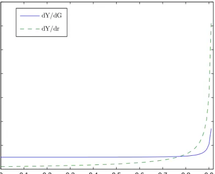
rL, in the case that µis large; in fact, ϑr (the multiplier dY /dr plotted in Figure 2)
becomes unboundedly large as µapproaches ¯µ. Under such circumstances, it can be highly desirable to stimulate aggregate demand by increasing the level of government purchases.
For levels of government purchases up to Gcrit, (4.9) implies that each additional
dollar spend by the government increases GDP by ϑG dollars.28 Increases in
govern-26Note that if, as in Eggertsson and Woodford (2003), it is assumed that the central bank pursues
a strict zero inflation target as long as this is consistent with the zero lower bound, then the zero lower bound necessarily binds at dates t < T if ˆGL = 0,as long as rL <0. The values computed
here for the multipliers dYL/drL anddYL/dGL are the same under that simpler hypothesis.
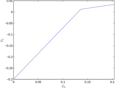
27As illustrated in Figure 1, output may nonetheless exceed its steady-state level; for the parameter
values assumed in the figure, YL exceeds ¯Y (so that ˆYL>0) for values ofGL nearGcrit, though the
output gap remains negative, because the increased government purchases increase the “natural” level of output.
28Note that this multiplier is calculated using approximations to the model structural equations
that have been log-linearized around the zero-inflation steady state, as in Eggertsson (2009) and Christiano et al. (2009). However, the case considered here is necessarily some distance from that steady state, so that the derivatives used need not yield a correct multiplier. (The multiplier computed here is correct only in the case that rL is a sufficientlysmall negative quantity, so that
πL and ˆYL remain close to zero when ˆGL = 0.) Braun and Waki (2010) find that log-linearization
around the zero-inflation steady state can substantially exaggerate the size of the multiplier under realistic parameter values; but they still conclude on the basis of their nonlinear analysis that the
0 0.05 0.1 0.15 0.2 −0.3 −0.25 −0.2 −0.15 −0.1 −0.05 0 0.05 ˆ GL ˆYL
Figure 1: Output as a function of the level of government purchases during the period (t < T) in which credit spreads remain elevated. A “Great Depression” shock is assumed, parameterized as in Eggertsson (2009).
ment purchases beyond that level result in even higher levels of GDP, though the increase per dollar of additional government purchases is smaller, as shown in Figure 1, owing to the central bank’s increase in interest rates in accordance with the Taylor rule. (Figure 1 plots ˆYL as a function of ˆGL, for the numerical parameter values
proposed by Eggertsson, 2009.29 Under these parameter values,Gcrit is reached when
multiplier is well above 1.
29Eggertsson chooses parameter values to fit the size of the contraction experienced by the U.S.
economy during the Great Depression. According to his modal parameter estimates (for a quarterly model), β = 0.997, κ = 0.00859, σ = 0.862, and Γ = 0.425.The shock required to account for the size of the contraction during the Depression is one under which rL = −0.010 (minus 4 percent
per annum) and µ = 0.903 (an expected mean duration a little over 10 quarters); the response coefficients for monetary policy are assumed to be φπ = 1.5, φy = 0.25. (The justification of these parameter values is discussed in greater detail in Denes and Eggertsson, 2009). Note that because I use a simpler model of the labor market in the current exposition, κ is not the same function of underlying parameters in (3.10) above as in Eggertsson’s paper. Here I parameterize the model so
government purchases exceed their steady-state value by 13.6 percent of steady-state GDP.30) For values G
L > Gcrit, the multiplier is no longer ϑG, but instead the
co-efficient γy defined in (3.17), where the persistence parameter ρ is now replaced by
µ.31
It follows from (4.7) that the multiplierdYL/dGL=ϑG for government purchases
up to the level ˆGcrit is necessarily greater than 1 (for any µ >0). The reason is that,
given that the nominal interest rate remains at zero in periods t < T, an increase in
GL,which increasesπL, accordingly increases expected inflation (given some positive
probability of elevated credit spreads continuing for another period), and so lowers
the real rate of interest.32 Hence monetary policy is even more accommodative than
is assumed in the benchmark analysis in section 2, and the increase in aggregate output is correspondingly higher.
The degree to which the multiplier exceeds 1 in this case can, in principle, be quite considerable. In fact, for any given values of the other parameters, the multiplier while the policy rate remains at the zero bound can be unboundedly large, for a sufficiently value of the persistence parameter µ. Figure 2 plots the multiplier as a function of µ, holding the other model parameters fixed at the values used by Eggertsson (2009). The figure illustrates something that can be observed from (4.7) to hold quite generally: the multiplier is monotonically increasing in µ,and increases
that the value of κis the same as in Eggertsson’s paper, meaning that implicitly the value ofαis larger than the value assumed by Eggertsson. The difference in the values assumed for α has no consequences for the multiplier calculations discussed here.
30In drawing the figure, I have also assumed that the credit spread is zero in the “normal” state,
so that ¯r=−logβ.Allowing for a small positive credit spread in this state would raise the value of
Gcrit.
31Under Eggertsson’s parameter values, this quantity is equal only to 0.3. (Note that this is a case
in which, when the central bank is not constrained by the zero bound, the multiplier under a Taylor rule that responds to detrended output is actually lower than the neoclassical benchmark; for under Eggertsson’s parameter values, Γ = 0.4.) Under the alternative hypothesis that the central bank implements a strict zero inflation target, except when prevented by the zero bound, the multiplier above the critical level of government purchases is equal to Γ.If instead the central bank follows a Taylor rule of the form (3.11), the multiplier beyond the critical level of government purchases is given by (3.16).
32Note that the increase in expected inflation referred to here is actually a reduction in the
expected rate of deflation. For all levels of government purchases below Gcrit, the output gap
remains negative (output remains below the flexible-price equilibrium level), and it is expected to be non-positive in all future periods as well, so that a negative rate of inflation is implied by (3.10).
0 0.1 0.2 0.3 0.4 0.5 0.6 0.7 0.8 0.9 0 2 4 6 8 10 12 14 µ dY/dG dY/dr
Figure 2: Derivatives of YL with respect to the values of rL and GL, for alternative
assumed degrees of persistenceµof the financial disturbance. Other parameter values are taken from Eggertsson (2009).
without bound as µ approaches ¯µ. The figure also indicates that the multiplier is in general not too much greater than 1, except if µ is fairly large. However, it is important to note that the case in which µ is large (in particular, a large fraction of ¯
µ) is precisely the case in which the multiplier dYL/drL is also large, which is to say,
the case in which a moderate increase in the size of credit spreads can cause a severe output collapse.33
Thus increased government purchases when interest rates are at the zero bound should be a powerful means through which to stave off economic crisis precisely in those cases in which the constraint of the zero lower bound would otherwise be most crippling — namely, those cases in which there is insufficient confidence that the disruption of credit markets will be short-lived. For example, in Eggertsson’s numerical example, a contraction of the size experienced during the Great Depression
occurs as a result of a disturbance with a persistence coefficient of µ = 0.903; in the case of this kind of disturbance, his parameter values imply a multiplier of 2.3. Christiano et al. (2009) similarly find that a multiplier above 2 is possible at the zero lower bound, in the context of a more complex New Keynesian model that is estimated to match a large number of features of postwar U.S. data.
Evidence on the effects of defense spending during the 1930s suggest that substan-tial multipliers of this kind may indeed be possible during circumstances like those of the Great Depression. For example, Almunia et al. (2010) estimate panel vector autoregressions using data from 27 countries for the period 1925-1939, and look at the response to innovations in defense purchases, taken to represent exogenous changes in government purchases; depending on the specification used, they find a multiplier during the year of the innovation of either 2.5 (their Figure 14) or 2.1 (their Figure 19). Gordon and Krenn (2010) similarly find a multiplier greater than 1 for the effects of innovations in government purchases on U.S. real GDP during the military buildup between 1940:Q2 and 1941:Q4. It is arguable that these relatively high multipliers for defense purchases during the Depression, relative to those found by studies of the effects of defense purchases at other times (e.g., those summarized in Hall, 2009), reflect a greater degree of monetary accommodation under Depression circumstances than has been typical of other military buildups.34
4.2
Importance of the Duration of Fiscal Stimulus
Cogan et al. (2010) instead find that a leading empirical New Keynesian model of the U.S. economy predicts small multiplier effects of increased government purchases during a situation in which the zero lower bound is assumed to bind. For example, when Coganet al. consider the effect of a permanent increase in government purchases of 1 percent of GDP, they find an increase in GDP of only 1.0 percent in the first quarter, which falls to only 0.6 percent by the end of the second year (the period over which they assume that the federal funds rate rate remains at zero), and to only 0.4 percent after four years. In the case of an assumed path of government purchases intended to mimic projected expenditure under the February 2009 U.S. federal stimulus package, their model implies an increase in GDP substantially smaller
34In fact, the VAR results of Almunia et al. show central-bank discount rates being reduced,
than the increase in government purchases in all quarters, and hence a particularly modest increase in output during the first year of their simulation.
What accounts for the difference with the large multiplier obtained at the zero bound by Eggertsson (2009)? While the empirical model used by Cogan et al. is substantially more complex, this is probably not the most important difference in their analysis.35 The crucial difference is that the calculations above assume an
increase in government purchases that lasts precisely as long as credit spreads are elevated, and hence precisely as long as the zero lower bound is a binding constraint, following which period Gt = ¯G again each period; Cogan et al. instead consider
increases in government purchases that are initiated at a time when interest rates are zero, but that extend much longer than the period over which the interest rate is assumed to remain at zero.
In our simple model as well, the increase in output is predicted to be much smaller if a substantial part of the increased government purchases are expected to occur after the zero lower bound ceases to bind. For as explained above, once interest rates are determined by a Taylor rule, a higher level of government purchases should crowd out private spending (raising the marginal utility of private expenditure), and may well cause lower inflation as well.36 But the expectation of a higher marginal
utility of expenditure and of lower inflation in the event that credit spreads normalize in the following period both act as disincentives to private expenditure while the nominal interest rate remains at zero. Hence while there is a positive effect on output during the crisis of increased government purchases at dates t < T,an anticipation of increased government purchases at dates t ≥T has a negative effect on output prior to date T.
A simple calculation can illustrate this. Suppose that instead of the two-state Markov chain considered above, there are three states: after the “crisis” state (in which rnet
t =rLand ˆGt = ˆGL) ends, there is a probability 0< λ <1 each period that
government purchases will remain at their elevated level ( ˆGt = ˆGL), even though
rnet
t = ¯r, though with probability 1− λ each period the economy returns to the
35The empirical model considered by Christianoet al. (2009) has a structure very similar to the
one used by Cogan et al., yet Christiano et al. obtain multipliers well in excess of 1 for a policy experiment similar to the one analyzed above.
36Both things occur in the case of the Eggertsson (2009) parameter values explained in footnote