the Context of Data Mining
Aliya Aleryani1,2, Dr. Wenjia Wang1and Dr. Beatriz De La Iglesia1
1
University of East Anglia, Norwich NR4 7TJ, UK 2
King Khalid University, Abha 61421, SA
Abstract. Missing data is an issue in many real-world datasets yet ro-bust methods for dealing with missing data appropriately still need devel-opment. In this paper we conduct an investigation of how some methods for handling missing data perform when the uncertainty increases. Using benchmark datasets from the UCI Machine Learning repository we gen-erate datasets for our experimentation with increasing amounts of data Missing Completely At Random (MCAR) both at the attribute level and at the record level. We then apply four classification algorithms: C4.5, Random Forest, Na¨ıve Bayes and Support Vector Machines (SVMs). We measure the performance of each classifiers on the basis of complete case analysis, simple imputation and then we study the performance of the algorithms that can handle missing data. We find that complete case analysis has a detrimental effect because it renders many datasets in-feasible when missing data increases, particularly for high dimensional data. We find that increasing missing data does have a negative effect on the performance of all the algorithms tested but the different algorithms tested either using preprocessing in the form of simple imputation or handling the missing data do not show a significant difference in perfor-mance.
Keywords: missing data, classification algorithms, complete case anal-ysis, single imputation.
1
Introduction
Many real-world datasets have missing or incomplete data [24]. Since the ac-curacy of most machine learning algorithms for classification, regression, and clustering is affected by the completeness of datasets, processing and dealing with missing data is a significant step in the Knowledge Discovery and Data Mining (KDD) process. Some strategies have been devised to handle incomplete data as explained in [8, 14, 5]. In particular, for regression, where missing data has been more widely studied (e.g. [9]), multiple imputation has shown advan-tage over other methods [22, 23]. However, much work is still needed to solve this problem in the context of data mining tasks and multiple imputation in particular needs some research to show if it is equally applicable to data mining. Before we investigate multiple imputation and data mining, which is our long term aim, in this research we want to deliver a thorough understanding of
how the different methods for handling missing data affect the accuracy of data mining algorithms when the uncertainty increases, i.e. the amount of missing data increases. We create an experimental environment using the university of California Irvine (UCI) Machine learning repository [13], by removing data from a number of UCI datasets completely at random (MCAR). We select increasing number of attributes at random to remove data from and we also increase the number of records at random from which we remove data in the attributes se-lected. Therefore, we produce a number of experimental datasets which contain increasing amounts of data MCAR.
Researchers have used a number of different methods to treat missing data in the data preprocessing phase. In this paper, we study the performance of classification algorithms in the context of increasing missing data under different pre-processing scenarios. In particular, we investigate how increasing the amount of missing data affects the performance for complete case analysis, and single imputation for a number of classification algorithms. We also compare that to the performance of algorithms with an internal mechanisms to handle the missing data, such as C4.5, and Random Forest.
The rest of this paper is organised as follows: Section 2 presents the problem of missing data and Section 3 presents the mechanisms used in Data Mining to address the problem. The methods used in our paper to set up our experimental environment are discussed in Section 4. Section 5 analyses the results. A discus-sion of the results is in Section 6. Finally, Section 7 presents our concludiscus-sions.
2
The problem of missing data
Little and Rubin [14] have defined missing data based on the mechanism that generates the missing values into three main categories as follows: Missing Com-pletely at Random (MCAR), Missing at Random (MAR), and Missing not at Random (MNAR). Missing Completely at Random (MCAR) occurs when the probability of an instance missing for a particular variable is independent from any other variable and independent from the missing data so missing is not re-lated to any factor known or unknown in the study. Missing at Random (MAR) occurs when the probability of an instance having a missing value for an at-tribute may depend on the known values but not on the value of the missing data itself. Missing not at Random (MNAR) occurs when the probability of the instance having a missing value depends on unobserved values. This is also termed a nonignorableprocess and is the most difficult scenario to deal with. In this paper we focus on generating missing data using the MCAR mechanism. Further work will investigate the other mechanisms.
Horton et al. [9] have further categorized the patterns of missing data into monotone and non-monotone. They state that the patterns are concerned with which values are missing, whereas, the mechanisms are concerned with why data is missing. We can state that we have monotone patterns of missing data if the same data points have missing values in one or more features. We focus in this study on non-monotone missing data.
3
Dealing with Missing Data
In practice, there are three popular approaches that are commonly used to deal with incomplete data:
1. Complete Case Analysis:This approach is the default in many statistical packages but should be only used when missing is under MCAR [14]. All incomplete data points are simply omitted from the dataset and only the complete records are used for model building [14]. The approach results in decreasing the size of data and the information available to the models and may also bias the results [20]. Tabachnick and Fidell [21] assumed that both the mechanisms and the patterns of missing values play a more significant role than the proportion of missing data when complete case analysis is used. 2. Imputation: Imputation means that missing values are replaced in some way prior to the analysis [14]. Mean or median imputation is commonly used with numerical instances and mode imputation with the nominal instances. Such simple imputation methods have been criticized widely [4, 18], because they do not reflect the uncertainty in the data and may introduce bias in the analysis. On the other hand, multiple imputation [17], a more sophis-ticated method, replaces missing values with a number of plausible values which reflect the uncertainty although the technique may have higher com-putational complexity. A method for combining the results of the analysis on multiple datasets is also required. For regression analysis, Rubin [17] defined some rules to estimate parameters from multiple imputation analysis. For application to data mining, good methods for pooling the analysis may be required.
3. Model Approach:A number of algorithms have been constructed to cope with missing data, that is, they can develop models in the presence of in-complete data. The internal mechanisms for dealing with missing data are discussed in the context of the algorithms used in this study.
3.1 The Classification Algorithms and Missing Data
We focus on the following well known classification algorithms, some of which have been identified as top data mining algorithms [25]: Decision Trees (C4.5), Na¨ıve Bayes (NB), Random Forest (RF) and Support Vector Machines (SVMs). Further, we will explain how different algorithms and their implementations in
Weka, our platform of choice, can treat missing values at both the building and the application phase.
C4.5 is one of the most influential decision trees algorithm. The algorithm was modified by Quinlan [15, 16] to treat missing data usingfractional method in which the proportion of missing values of an attribute are used to modify the
Information gain andSplit ratio of the attribute’sGain ratio. After making the decision for splitting on an attribute with the highest gain ratio, any instance with missing values of that attribute is split into several fractional instances which may travel down different branches of the tree. When classifying an in-stance with missing data, the inin-stance is split into several fractional inin-stances
and the final classification decision is a combination of the fractional cases [6]. We use theWeka implementation, J48, which uses the fractional method [7].
Na¨ıve Bayes algorithm is based on the Bayes theorem of probabilities using the simplification that the features are independent of one another. Na¨ıve Bayes ignores features with missing values thus only the complete features are used for classification [2, 11]. Therefore, it uses complete case analysis instead of handling missing data internally.
Random Forest is an ensemble algorithm which produces multiple decision trees and can be used for classification and regression. It is considered as a robust algorithm and produces high classification accuracies. This is because random forest splits training samples to a number of subsets then builds a tree for each subset, rather than building one tree [1] and combines their decision. Random Forest, uses the fractional method [1, 10] for missing data in a similar manner to C4.5. The implementation of the algorithm in Weka also uses the fractional method as in C4.5 algorithm.
SVMs are used for binary classification and can be extended to higher di-mensional datasets using the Kernel function [19]. SVMs maximize the margin between the separating hyperplane and the classes. The decision function is de-termined by a subset of training samples which are the support vectors. We use a Weka implementation called SMO (Sequential Minimal Optimization), a modification of the algorithm that solves the problem of Quadratic Program-ming (QP) when training SVMs in higher dimensions without extra storage or optimization calculations. Although SVMs do not deal with missing values [12], the SMO implementation performs simple imputation by globally replacing the missing values with the mode if the attribute is nominal or with the mean if the attribute is continuous [7].
4
Methods
For our study, a collection of 17 benchmark datasets are collected from UCI machine learning repository [13]. The datasets have different sizes and feature types (numerical continuous, numerical integer, categorical and mixed) as shown in Table 1. None of the datasets have missing values in their original form so this enables us to study how missing data affects the accuracy and performance of classification algorithms.
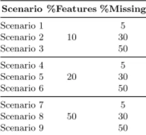
Data values are then removed completely at random as follows to generate increasing amounts of missing data. First, 10% (then 20%, 50%) of the attributes are randomly selected then missing values are artificially generated by removing values randomly in 5%, 30% and 50% of the records, respectively. As a result, nine artificial datasets are produced for each of the original datasets with mul-tiple levels of missing data. In total, we have 153 datasets. Table 2 summarises the experimental scenarios artificially created.
For testing the models, 10-fold cross-validation was used and performed 10 times. All results reported represent the average of the 10 experiments with 10-fold cross-validation.
Table 1.The details of the datasets collected for the experiments.
No. Dataset #Features #Instances #Classes Feature Types
1 Post-Operative Patient 8 90 4 Integer, Categorical 2 Ecoli 8 336 8 Real
3 Tic-tac-toe 9 958 2 Categorical 4 Breast Tissue 10 106 6 Real
5 Statlog 20 1000 2 Integer, Categorical 6 Flags 30 194 8 Integer, Categorical 7 Breast Cancer Wisconsin 32 569 2 Real
8 Chess 36 3196 2 Categorical 9 Connectionist Bench 60 208 2 Real 10 Spect 69 287 2 Categorical 11 Hill Valley 101 606 2 Real 12 Urban Land Cover 148 168 9 Integer, Real 13 Epileptic Seizure Recognition 179 11500 5 Integer, Real 14 Semeion 256 1593 2 Integer 15 LSVT Voice Rehabilitation 309 126 2 Real 16 HAR Using Smartphones 561 10299 6 Real 17 Isolet 617 7797 26 Real
Table 2.Experimental scenarios with missing data artificially created.
Scenario %Features %Missing
Scenario 1 10 5 Scenario 2 30 Scenario 3 50 Scenario 4 20 5 Scenario 5 30 Scenario 6 50 Scenario 7 50 5 Scenario 8 30 Scenario 9 50
In the complete case analysis, all the incomplete records are omitted. This often results in datasets that are too sparse to be used for classification. The datasets that are left with enough records for classification are considered feasi-ble.
To test simple imputation, the numerical attributes are replaced with their mean and the categorical attributes with their mode. Then the produced datasets after imputation are used for classification model building.
We use the classifiers: J48, Na¨ıve Bayes, RandomForest and SMO imple-mented in Weka with their default options for classifying the data. We use the classification accuracy as a metric for our experiments. To further compare per-formance of the classifiers, we compute the average of the percentage difference in accuracy between a classifier obtained with the original (complete) datasets and the datasets with increasing missing data as follows:
%Diff = (((Acc Scei−Acc Orgj)/Acc Orgj)∗100) (1)
whereAcc Sceirepresents the classifier accuracy for a specific scenario, in our
experiment we have 9 scenarios, andAcc Orgj represents the classifier accuracy
We perform two different statistical tests when evaluating the performance of classifiers over the datasets as follows:
1. When comparing differences in accuracy for each scenario we first use Wilcoxon Signed Rank test with a significance level atα= 0.05.
2. We then compare multiple classifiers over multiple datasets using the method described by Demˇsar [3], including the Friedman test and the post hoc Ne-menyi test which is presented as a Critical Difference diagram, with a sig-nificance level ofα= 0.05.
5
Results
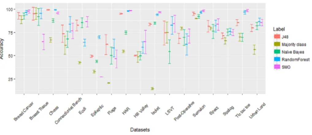
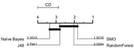
Fig. 1 shows the average accuracy of classifiers and standard deviation (as error bars) for each of the original complete datasets along with the baselinemajority class model accuracy. Models perform better than the baseline in most of the datasets except Post-Operative Patient, Breast Tissue, Spect, and LSVT Voice Rehabilitation, where default accuracy is similar or slightly better than that obtained by the models. We use the Friedman test for statistical differences. The resulting p-value < 0.05, so we proceed with Nemenyi test. The Critical Difference diagram for the Nemenyi test is shown in Fig. 2. The Figure illustrates that SMO and RandomForest behave better than J48 and Na¨ıve Bayes although there is no statistical differences within each group.
Fig. 1.The average accuracy of classifiers and standard deviation (as error bars) for each of the original (complete) datasets along with majority class.
5.1 Complete Case Analysis
The datasets that are not feasible for classification after removing missing records are marked with 7 whereas the feasible are marked with 3 as shown in Ta-ble 3. Datasets are ordered by increasing number of attributes (dimensionality)
Fig. 2.Critical Difference diagram shows the statistical difference between the classi-fiers. The bold line connecting classifiers means that they are not statistically different.
and then number of records. Only two low dimensional datasets are feasible for classification in all scenarios: Ecoli and Tic-tac-toe. In contrast, datasets with increasing dimensionality are not feasible for classification when increasing the amount of missing data due to widespread sparsity. For example, Hill Valley, UrbanLandCover, Epileptic Seizure Recognition, Semeion, LSVT Voice Reha-bilitation, HAR Using Smartphones and Isolet all become mostly infeasible.
Table 3. The artificial datasets with different scenarios of missing data that are not feasible when applying the classification algorithms are marked with7.
Scenario Dataset 1 2 3 4 5 6 7 8 9 Post-Operative Patient 3 3 3 3 3 3 3 3 7 Ecoli 3 3 3 3 3 3 3 3 3 Tic-tac-toe 3 3 3 3 3 3 3 3 3 Breast Tissue 3 3 3 3 3 3 3 3 7 Statlog 3 3 3 3 3 3 3 3 7 Flags 3 3 3 3 3 7 3 7 7
Breast Cancer Wisconsin 3 3 3 3 7 7 3 7 7
Chess 3 3 3 3 3 3 3 7 7
Connectionist Bench 3 3 7 3 7 7 3 7 7
Spect 3 3 3 3 3 7 3 7 7
Hill Valley 3 3 7 3 7 7 3 7 7
UrbanLandCover 3 7 7 3 7 7 7 7 7
Epileptic Seizure Recognition3 3 7 3 7 7 3 7 7
Semeion 3 7 7 3 7 7 7 7 7
LSVT Voice Rehabilitation 3 7 7 7 7 7 7 7 7
HAR Using Smartphones 3 7 7 3 7 7 7 7 7
Isolet 7 7 7 7 7 7 7 7 7
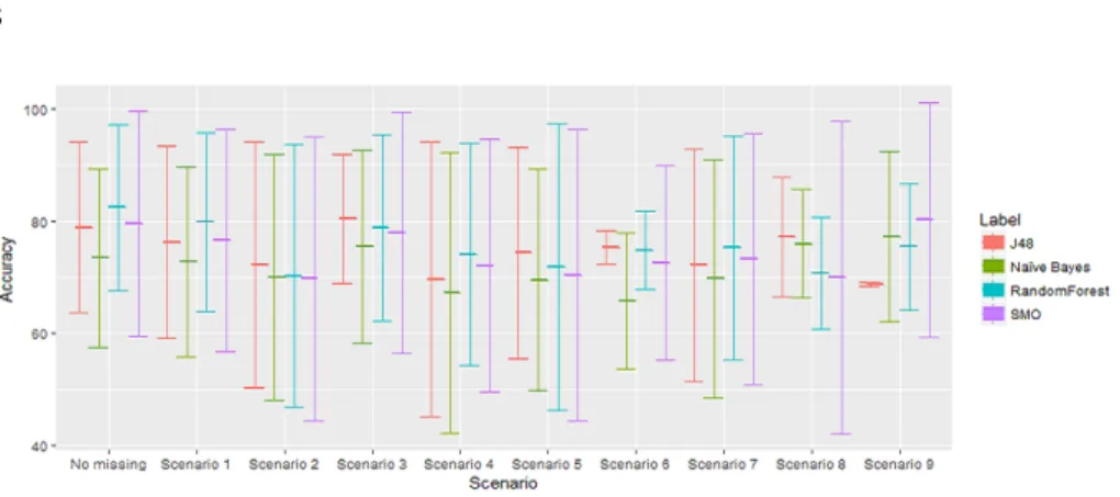
Fig. 3 illustrates the average accuracy of the classifiers and standard deviation for the datasets that are feasible for classification. In scenario 1, the average and the standard deviation are nearly equal to those on the original data. However, with a decreasing number of feasible datasets, the standard deviation increases and the classifiers’ performance deteriorate as we increase missing data.
Table 4 shows the average %Diff in accuracy between classifiers obtained with the original (complete) data and the datasets with increasing missing data for the different data handling approaches and algorithms. For complete case analysis, the deterioration in accuracy reached more than 18% for J48, RF, and SMO in different scenarios. However, Na¨ıve Bayes behaved better gaining 2% in
Fig. 3.The average accuracy of classifiers and standard deviation (as error bars) for all artificial datasets in all scenarios of missing data including the original (complete) datasets when applying complete case analysis.
some scenarios. We do not produce statistical analysis due to the small number of datasets that produce a feasible classification with complete analysis. 5.2 Simple Imputation
Table 4 also shows the average of all the percentage differences in accuracy (%Diff) between a classifier obtained with the original (complete) datasets and the imputed data for each scenario and each algorithm. %Diff increases when missing data increases in all classifiers, however simple imputation performs much better than complete case analysis. Accuracy decreased in a small range between [-0.54,-5.59] for J48 and by -6.94% for RandomForest in the worst case. For Na¨ıve Bayes, the differences with the original data where smaller with a maximum deterioration of -2.67%. SMO sees deteriorations of up to 5.71% in the scenarios of most missing data. We applied the Wilcoxon Signed Rank test to check statistical significance over the differences. Significant values are marked with * and tend to be those for the higher scenarios, except for SMO where the differences are more often statistically significant. From this we can conclude that simple imputation may work well for low amounts of missing data, and is beneficial over complete case analysis, but performance deteriorates significantly when the amount of missing data increases.
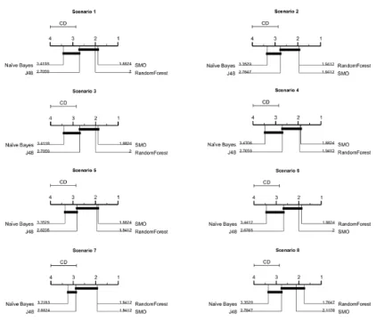
We also applied the Friedman test described by Demˇsar [3] and found statisti-cally significant differences over multiple datasets in all scenarios except scenario 9 so we proceeded with the Nemenyi Test. We perform the post test between the classifiers over the imputed datasets for each scenario separately. The resulting Critical Difference diagrams in most scenarios in Fig. 4 show that RandomForest and SMO outperform J48 and Na¨ıve Bayes. Random Forest seems to outperform SMO as the amount of missing data increases but not significantly. There is no statistical difference between RandomForest, SMO, and J48 in most scenarios. Overall, RandomForest was the most accurate classifier when the uncertainty increases and Na¨ıve Bayes was the worst.
Table 4.Average % Diff in Accuracy with respect to complete data. Wilcoxon Signed Rank is used to test statistical significance with significant results marked by *.
Complete Case Simple Imputation Algorithms Only Scenario # J48 NB RF SMO J48 NB RF SMO J48 NB RF SMO Scenario 1 -3.27 0.26 -2.28 -2.07 -0.54* 0.01 -0.10 -0.57* -0.19 0.05 -0.41* -0.59* Scenario 2 -6.88 -3.92 -12.08 -8.00 -0.57 0.11 -0.82 -1.34 -0.38 0.22 -0.72 -1.38 Scenario 3 -1.82 -3.81 2.82 -4.04 -0.96* -0.30 -1.10* -2.03* -0.64 -0.48 -1.33* -2.04* Scenario 4 -11.50 -9.43 -14.29 -6.75 -0.83* -0.17 -0.56 -1.05* -0.53 0.00 -0.66* -1.08* Scenario 5 -8.99 -10.01 -11.26 -12.97 -1.24* -0.14 -1.62* -2.26* -0.56 0.00 -1.50* -2.31* Scenario 6 -8.35 -16.03 -6.58 -12.03 -1.62* -0.84 -2.31* -3.07 -0.99 -0.78 -1.85* -2.95 Scenario 7 -6.80 -4.11 -4.27 -1.14 -1.27* 0.22 -2.03* -1.39 -1.02* 0.10 -1.94* -1.25 Scenario 8 -3.64 -2.30 -8.75 -14.04 -3.86* -1.41 -5.11* -5.11* -2.56* -1.15* -4.78* -5.04* Scenario 9 -18.17 -2.10 -4.31 -13.83 -5.59* -2.67* -6.94* -5.71* -3.95* -1.42* -5.85* -5.82*
Fig. 4.Critical Difference diagrams show the statistical significant differences between classifiers using simple imputation. We exclude scenario 9 where all classifiers are not statistically different with the Friedman test.
5.3 Building models with missing data
In Section 3.1 we discussed that some of this algorithm have their own ways of dealing with missing data. We therefore pass all the data including missing data to the algorithms without preprocessing. We again compare (%Diff) in ac-curacy between a classifier obtained with the original (complete) datasets and the models built with missing data and show results in Table 4 with statistically significant differences marked by *. %Diff increases when missing data increases in all classifiers. However, for J48 in most of scenarios the deterioration is within
a small range [-0.19%,-3.95%] and similarly for RandomForest [-0.41%,-5.85%]. Na¨ıve Bayes only ignores the missing values when computing the probability and the differences ranged between [+0.22%,-1.42]. SMO uses (mean/mode) im-putation so behaves similarly to the imputed data performance in Table 4. In scenarios 8 and 9, the accuracy of all classifiers are statistically different from the classifiers’ accuracy for the original datasets. Thus, the capabilities of classifiers dealing with missing data seem to deteriorate when the ratio of missing data increases.
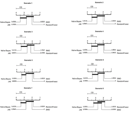
As before we apply the Friedman test and Nemenyi post test. The resulting Critical Difference diagrams in most scenarios show that RandomForest and SMO outperform J48 and Na¨ıve Bayes. However, there is no statistical difference between all classifiers in scenario 9 whereas no statistical significant between RandomForest, SMO and J48 and between Na¨ıve Bayes and J48. SMO was the most accurate classifier in the first six scenarios, however, when increasing missing data RandomForest outperforms other classifiers and Bayes was the worst in all scenarios. Fig. 4 represents the Critical Difference diagrams of all scenarios.
Fig. 5. Critical difference diagrams show the statistical difference between classifiers with no preprocessing of missing data, excluding scenario 9 where all classifiers are not statistically different.
6
Discussion
With complete data, Na¨ıve Bayes and J48 perform worse than SMO and Ran-dom Forest. Complete case analysis results in many datasets becoming infeasible for analysis due to sparsity of the data for the algorithms we tested, thus it is not recommended if missing values are spread among records in high dimen-sional data. Simple imputation works well for low amounts of missing data but not when the amount of missing data increases substantially (scenarios 8,9), as the performance of all classifiers becomes statistically significantly worse than classifying with complete data. RandomForest and SMO behave better than J48 and Na¨ıve Bayes in all scenarios (including when complete data is available). The capability to cope with missing data for RandomForest by using fractional method when uncertainty increases seems to outperform the SMO handling of missing data using mean/mode but not significantly.
7
Conclusion
Accuracy deteriorates for most classifiers when increasing percentages of miss-ing data are encountered. Complete case analysis is not recommended if missmiss-ing values are spread among (Features/Records) in high dimensional data. Simple imputation may help when a dataset has low ratio of missing values but not with increasing uncertainty. When applying the algorithms without preprocessing, again the trend is for some deterioration in performance with increasing missing data with those differences becoming statistically significant for the higher sce-narios. So overall, we expect models to become worse as the amount of missing data increases though different algorithms do not perform significantly differ-ently under those scenarios. As future work, we will expand on our imputation to include multiple imputation that combines models generated from multiple imputed datasets with data ensemble techniques to improve the performance of data mining classification algorithms for data with missing values.
References
1. Leo Breiman. Random forests. Machine learning, 45(1):5–32, 2001.
2. Xiaoyong Chai, Lin Deng, Qiang Yang, and Charles X Ling. Test-cost sensitive naive bayes classification. InData Mining, 2004. ICDM’04. Fourth IEEE Interna-tional Conference on, pages 51–58. IEEE, 2004.
3. Janez Demˇsar. Statistical comparisons of classifiers over multiple data sets.Journal of Machine learning research, 7(Jan):1–30, 2006.
4. Mark Fichman and Jonathon N Cummings. Multiple imputation for missing data: Making the most of what you know. Organizational Research Methods, 6(3):282– 308, 2003.
5. Pedro J Garc´ıa-Laencina, Jos´e-Luis Sancho-G´omez, and An´ıbal R Figueiras-Vidal. Pattern classification with missing data: a review. Neural Computing and Appli-cations, 19(2):263–282, 2010.
6. Sachin Gavankar and Sudhirkumar Sawarkar. Decision tree: Review of techniques for missing values at training, testing and compatibility. InArtificial Intelligence, Modelling and Simulation (AIMS), 2015 3rd International Conference on, pages 122–126. IEEE, 2015.
7. Theofilis George-Nektarios. Weka classifiers summary. Athens University of Eco-nomics and Bussiness Intracom-Telecom, Athens, 2013.
8. Jerzy W Grzymala-Busse and Ming Hu. A comparison of several approaches to missing attribute values in data mining. In International Conference on Rough Sets and Current Trends in Computing, pages 378–385. Springer, 2000.
9. Nicholas Horton and Ken P. Kleinman. Much ado about nothing: A comparison of missing data methods and software to fit incomplete data regression models. The American Statistician, 61:79–90, 2007.
10. Mohammed Khalilia, Sounak Chakraborty, and Mihail Popescu. Predicting disease risks from highly imbalanced data using random forest. BMC medical informatics and decision making, 11(1):51, 2011.
11. Ron Kohavi, Barry Becker, and Dan Sommerfield. Improving simple bayes. In Proceedings of the European Conference on Machine Learning. Citeseer, 1997. 12. Sotiris B Kotsiantis, I Zaharakis, and P Pintelas. Supervised machine learning: A
review of classification techniques. Emerging artificial intelligence applications in computer engineering, 160:3–24, 2007.
13. M. Lichman. UCI machine learning repository.http://archive.ics.uci.edu/ml, 2013.
14. Roderick JA Little and Donald B Rubin. Statistical analysis with missing data. John Wiley & Sons, 2014.
15. J Ross Quinlan. C4. 5: programs for machine learning. Elsevier, 2014.
16. J Ross Quinlan et al. Bagging, boosting, and c4. 5. In the Association for the Advancement of Artificial Intelligence (AAAI), Vol. 1, pages 725–730, 1996. 17. Donald B Rubin. Multiple imputation after 18+ years. Journal of the American
statistical Association, 91(434):473–489, 1996.
18. Judi Scheffer. Dealing with missing data.Research Letters in the Information and Mathematical Sciences, 3(1):153–160, 2002.
19. Bernhard Sch¨olkopf, Christopher JC Burges, and Alexander J Smola. Advances in kernel methods: support vector learning. MIT press, 1999.
20. Marina Soley-Bori. Dealing with missing data: Key assumptions and methods for applied analysis. Boston University School of Public Health, 2013.
21. Barbara G Tabachnick, Linda S Fidell, and Steven J Osterlind.Using multivariate statistics. Allyn and Bacon Boston, 2001.
22. Cao Truong Tran, Mengjie Zhang, Peter Andreae, Bing Xue, and Lam Thu Bui. Multiple imputation and ensemble learning for classification with incomplete data. InIntelligent and Evolutionary Systems: The 20th Asia Pacific Symposium, IES 2016, Canberra, Australia, November 2016, Proceedings, pages 401–415. Springer, 2017.
23. Geert JMG van der Heijden, A Rogier T Donders, Theo Stijnen, and Karel GM Moons. Imputation of missing values is superior to complete case analysis and the missing-indicator method in multivariable diagnostic research: a clinical example. Journal of clinical epidemiology, 59(10):1102–1109, 2006.
24. Ian H Witten, Eibe Frank, Mark A Hall, and Christopher J Pal. Data Mining: Practical machine learning tools and techniques. Morgan Kaufmann, 2016. 25. Xindong Wu, Vipin Kumar, J Ross Quinlan, Joydeep Ghosh, Qiang Yang, Hiroshi
Motoda, Geoffrey J McLachlan, Angus Ng, Bing Liu, S Yu Philip, et al. Top 10 algorithms in data mining. Knowledge and information systems, 14(1):1–37, 2008.