Integrating digitizing pen technology and machine learning with the Clock Drawing Test

(1)

Integrating Digitizing Pen

Technology and Machine Learning

with the Clock Drawing Test

by

Kristen Felch

Submitted to the Department of Electrical Engineering and Computer Science in Partial Fulfillment of the Requirements for the Degree of

Master of Engineering in Electrical Engineering and Computer Science at the Massachusetts Institute of Technology

February 2010

2010 Massachusetts Institute of Technology

All rights reserved.

/ '-.\

Introduction

Bringing technology to the medical field is a present-day challenge that attracts the efforts of both researchers and doctors. Recent innovations in software and hardware provide seemingly endless opportunities for the advancement of medical data collection and analysis, but progress is slowed by the necessary caution and regulation surrounding work in the medical field. This thesis addresses the movement of one particular technology into the medical domain, and describes the tools that have been built to support the application.

The technology in question is a digitizing ballpoint pen, which records its location on paper through time-stamped data points; the medical application is the Clock Drawing Test (CDT). The Clock Drawing Test has a long history of success in diagnosing patients with Alzheimer's, Parkinson's, and other neurodegenerative diseases, but is currently administered using paper, pen, and subjective rating scales. Is it possible to improve the accuracy of the CDT through standard-ization of the data collection and analysis procedures, using a digitizing ballpoint pen rather than the traditional pen?

Software has been developed that interacts with the new pen to record results of the CDT. The Clocksketch program is straightforward, in use requiring minimal training for doctors that use it to administer the CDT. However, in order to be truly embraced by the medical community, CDT administration with the digitizing pen should be easier than traditional methods. My first contribution outlined in this thesis was improving the algorithm that runs behind the scenes of the Clocksketch program, easing the process of data analysis.

A computerized version of the CDT must maintain the ease-of-use of its pen and paper prede-cessor, its primary advantage over more intrusive/complex diagnostic tests, while also creating opportunities for more rigorous data analysis and standardization of data collection. My second

(6)

contribution is the creation of a data analysis package, the MultiTool Data Analysis Package (MDA), which was developed to ease exploratory analysis of CDT output data. MDA has evolved to handle any input data of a specified format, but its features and functionality were chosen by predicting the demands of a future analyst working with CDT data.

At this point, the data collected by digitizing pens from the CDT is small in size compared to the expected influx of data over the next few months. However, the successful processing of our limited data using MDA indicates that the tool will be indispensable once data arrives on a larger scale. MDA's chief functionality includes automatic creation of input files for machine learning tools and a common launching platform for these tools. With the most popular machine learning tools at his fingertips, an analyst will easily be able to provide more rigorous analysis of CDT data than that of a doctor prior to use of the digitizing pen.

The digitizing ballpoint pen and supporting software are making their way into the medical domain because of the improvements they can offer on the traditional Clock Drawing Test. Data collection is improved through use of classification algorithms dealing with output of the digitizing pen. Because of the digital nature of the test, the most modern machine learning techniques can be used to analyze output from the CDT and add rigor and standardization to the process. This thesis explains exactly how the data collection and analysis phases of the CDT are improved upon in the new Clock Drawing Test.

(7)

2

Background

To understand the advantages of incorporating the digitizing pen technology with the traditional Clock Drawing Test, we look at the history and development of the CDT. We then explore the most current technology for digitizing pens, and how they can be used in a medical context.

2.1

The Clock Drawing Test

The Clock Drawing Test is a cognitive screening tool that has been in use for over 50 years, diagnosing patients with various dementias and other neurological disorders. It is a fairly simple test, requiring the patient to draw two clocks showing a given time. One of these clocks is drawn without any visual references, while for the second the patient is given an image to copy. Previous research has shown that the CDT has high potential for differentially diagnosing Alzheimer's and other neurological disorders. However, the current implementation is a pen-on-paper sketch that is viewed by doctors and ranked based on widely-varying scales. Instructions given to the patient, implementation of the copied clock, and even the ranking scale for clock drawings differ depending on where the test is administered.

The success of the traditional CDT in recognizing neurological disorders even with nonstandard-ized procedures suggests that it could become a very powerful tool when executed using modern technology. In a 1986 study at the University of Toronto, researchers first attempted to collect data to legitimize the use of the CDT as part of cognitive screening. They compared the results of the CDT to results from two other well-established screens of cognitive function, and found that the CDT could provide a simple and practical method of screening for mental disorder. (Shulman 136)

For this Toronto study, seventy-five subjects were selected from the inpatient and outpatient pop-ulations at the University of Toronto. Subjects were over the age of 65, and included subjects with mental disorders and healthy subjects. Three tests were administered to the patients- the

(8)

Clock Drawing Test, the Mini-Mental State Exam, and the Short Mental Status Questionnaire. In addition, a test to assess the subject's level of depression was administered. The MMSE is one of the most widely-accepted cognitive function tests, and is often used as a standard for screening. The SMSQ is a short 10-answer questionnaire that classifies scores of 7 or above as normal. In administering the CDT, subjects were given the outline of a clock and asked to complete it and set the time to three o'clock. The clocks were then analyzed by two independent raters, who ranked the clock with a number 1-5 based on a hierarchical classification of errors. There were about 20 errors that the rankers were asked to look for when assigning a number to the clock. (Shulman 136) The results of this study showed that the magnitude of error in the CDT is correlated to the error of the MMSE and the SMSQ. In other words, when a subject scores poorly on the CDT he or she is likely to score poorly on the other tests as well. The correlation coefficient between two tests is a measure of how the pattern in results of one test mimick the patterns seen in the other test. The correlation coeffcient of the CDT and MMSE was -. 65, and that of the CDT and SMSQ was -. 66. Correlation is negative since high scores on the CDT indicate impaired cognition while high scores on the other two tests indicate a healthy subject. As a result of this study, the CDT was established as a useful addition to the cognitive tests already in use. Since it is simple to administer, it can provide a quick screening measure before the MMSE is administered. (Shulman 139)

Division of the Clock Test

One of the next advances in the CDT involved dividing the test into two separate parts. In a study at the University of Texas in 1998(Royall 589), it was shown that separate clock tests could be used to differentiate between alternative cognitive impairments. The first test, CLOXI, requires the test subject to draw a clock without any visual guidance. It is meant to reflect the subject's performance in a novel situation, something referred to as executive control, since he or she is pre-sented with only a blank page and asked to draw a clock showing a particular time. Observations were made such as the order that the digits were drawn in and whether or not corrections were made along the way. CLOX2 involves giving the subject a clock to look at and asking them to copy it. This test is aimed more at examining the subject's visuospatial awareness than executive control. Correlation between these two separate CDTs was measured in comparison to MMSE and EXIT25, a common measure of executive control. (Royall 589)

This study determined that both MMSE and EXIT25 results were correlated with results from CLOXI, but only MMSE was correlated with CLOX2. This is as expected, since copying a clock

(9)

2.1 The Clock Drawing Test

does not require the same cognitive function as drawing from memory. In a comparative analysis between both CLOX tests and MMSE performance, it was concluded that the CLOX tests were able to correctly identify 81:3% of subjects who had Alzheimer's disease. This is compared to the 89:9% that a combination of EXIT25 and MMSE achieve. When looking at differential diagnosis between Alzheimer's subgroups, CLOX2 scores alone were able to discriminate between the sub-groups. Using a combination of CLOXI and CLOX2, performance on differentiating Alzheimer's subgroups was 91:9% correct. This was a remarkable result, since a combination of EXIT25 and MMSE did not perform as well. The conclusion drawn from this study was that a combination of two clock drawings would be a practical and reliable cognition test to be used by clinicians.

(Royall 591-3)

Rating Scales

One of the most notable differences across CDT usage is the scale or rating system that is used. Some tests rate out of 4, others 5 or 10, and some up to 30. Clearly comparisons between facilities, or even between doctors within one facility, would be very difficult with this variation.

The ranking methods for the two studies described above differed in nature and content. For the Toronto study, errors were classified into different levels and the clock was classified to match the highest error level found. The first level included small errors such as drawing the numbers outside rather than inside the circle, or drawing in helper lines to indicate spacing. The middle levels included things such as leaving out numbers or continuing numbering past 12. The fifth and worst level was the inability to make an attempt at drawing a clock. (Shulman 136) Thus, the clocks were ranked from 1 to 5.

The Texas study had rankings that ranged from 0 to 15. Rather than dividing errors into levels to classify the clock, a simple checklist of common errors was used. Each error that occurred was worth one point, totalling 15. Things such as the absence of all 12 numbers on the clockface, as well as the absence of a minute hand and an hour hand, were each worth one point. (Royall 592) In both of these ranking systems, low scores indicate a healthy patient.

Several papers have been written comparing alternate rating systems for the CDT. In one study performed in 2002, 63 clock drawings were rated using 5 different scales and the results compared:

(10)

" The Sunderland scoring method assigns a maximum of 10 points, but is based on the place-ment of the hour and minute hands.

e The Shulman method was the one used in the Toronto study, but was modified to have 6 categories of error rather than 5.

" The Clock Drawing Interpretation Scale (CDIS) awards a maximum of 20 points for the circle, hand placement, and presence and placement of numbers.

" The Glass method assigns a score of 0 if five main aspects are correct- circle formation, numbers aligned, all numbers included, hands aligned, and both hands identified. Half of a point is added if one of the above is partially correct, and one point if it is incorrect. (Richardson 170)

The conclusion of this study was that each of the scoring methods had significant correlation with the MMSE test, with the Sunderland scoring criteria having the highest correlation. More importantly, it was discovered that different classification methods worked better for diagnosing different diseases. With patients who had Alzheimer's disease, the Glass method had the highest correlation with MMSE. For patients with mixed dementia and multiinfarct dementia, the CDIS scoring criteria yielded the highest correlation with MMSE.

The study concluded that patients with mixed dementia are more likely to make time-setting mistakes than number-spacing errors. Therefore, they score better with the Glass and Shulman tests that do not depend on the clock hand placement.

These results suggest that a standardized method of classification that combines all of the measure-ments would help to differentially diagnose the different types of neurogenetic diseases. (Richard-son 171-2)

A similar investigation conducted in Australia in 2001 assessed different scoring criteria by inte-grating the area under the ROC curve. The ROC curve is created by mapping the relationship between the number of true positives and false positives for a given scoring criteria. A high area, between .7 and .9, indicates a useful criteria because it means that a high percentage of positives can be correctly identified without incurring a large number of false positives. The scoring methods that were examined in this study were those proposed by Mendez, Shulman, Sunderland, Watson, and Wolf-Klein. The Mendez criterion has 20 frequent errors that are assigned points, similar to the CDIS. The Watson method scores out of 7 based on number placement. The study showed that

(11)

2.2 Digitizing Pen Technology

the Shulman and Mendez methods give the largest area under the ROC curve, and predict demen-tia more accurately than the Sunderland and Watson methods. The Schulman method had both high sensitivity and high specificity, while the Watson method had high sensitivity but low speci-ficity. The researchers conclude that the Schulman method scores the best, but that CDTs should still not be used alone to diagnose dementia. Until a standardized scoring criteria is developed and much more testing is done, CDTs are not reliable enough to be used as stand-alone tests. (Storey)

One such method of standardizing the CDT is use of a digitizing ballpoint pen. If a standard procedure for collecting data can be established through distribution of a pen and supporting software, then CDT results across locations can be compared and analyzed. With more data available, analysts will have a better sense of the comparitive diagnostic value of the CDT. The next section will describe the digitizing ballpoint pen that will be incorporated into the CDT.

2.2

Digitizing Pen Technology

In order to digitize the process of drawing, two components are necessary- the digitizing pen and special paper upon which to draw.

The Paper

Special paper is required in order for a digitizing pen to be able to store information about the image being drawn. This paper uses the Anoto pattern, which provides a simple but very power-ful mechanism that identifies which physical page a pen is on as well as the writing and drawing movements made on the page. The pen would not be able to record anything without the pattern, and it is the pattern that makes it possible for the pen to know what you write and where you write.

The Anoto pattern consists of small dots (100 microns in diameter) arranged with a spacing of approximately 0.3 mm on a square grid. The dots are slightly displaced from the grid, each dot in one of four possible positions. The pattern is visible on plain paper, but faint enough so as to not interfere with drawing.

The Pen

We used the the Maxell DP-201 (R4.1) digitizing pen. This pen has a built-in camera, which takes digital snapshots of the pattern as the pen moves over the paper. The pen uses an infrared LED (light-emitting diode) to take the snapshots between 50 and 100 times per second. The camera

(12)

can determine its position only on paper with an Anoto pattern. The pen processes the snapshots by calculating its position on the page, and stores the snapshots in the form of pen stroke data (a set of time-stamped coordinates). (Anoto(A) 22)

With the combined capabilities of a digitizing pen and the Anoto patterned paper, it is possible for the CDT to be recorded in the form of time-stamped points. Armed with this capability, we are ready to see how the data analysis stage of the CDT has been revolutionized by the digitizing pen technology and supporting software.

(13)

3

The Data Collection Process

In order for the digitizing ballpoint pen to be successfully integrated into the Clock Drawing Test, it must provide advantages during administration of the test. If it is more difficult or time-consuming to administer the CDT using a digitizing pen, doctors will be hesitant to make any changes to their time-proven approach. For this reason, the current software that supports the pen must be improved to have higher digit recognition rate so that less input from doctors is required.

3.1

Status Quo

The digital Clock Drawing Test is administered in much the same way as the traditional CDT, by asking the patient to draw two separate clocks. The patient uses the Maxell digitizing pen, and draws the clocks on paper containing an Anoto pattern. A few changes have been made to the administration process to reflect use of the digitizing pen.

The test paper is divided into a right and a left half, and the left half is covered for the first portion of the test. The test administrator places a check mark in the upper right corner of the page to indicate that a new test is starting, then hands the pen to the patient, who draws the first clock on the (empty) right half of the page. The left half of the page is then uncovered to reveal an image of a clock. The patient copies the image on the left half of the page, and the administrator places a check mark in the bottom right corner of the page to indicate completion.

The software that supports use of the digitizing pen with the Clock Drawing Test is called the Clocksketch program. Once the patient has completed the test, the pen is returned to its base, which is connected to the computer. It is possible to run tests on several patients before the pen is connected to the computer and data is transferred. The maximum amount of data that the pen

(14)

can store is that from approximately 500 patients.

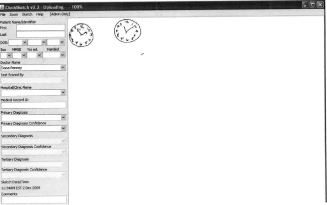
Once the pen has been connected to the computer, the Clocksketch program will automatically launch. The first test will be loaded, and images of the two clocks will appear in the center panel. The doctor will enter information including patient name, date of birth, sex, MMSE score, doctor name, and scorer name. Once this information is entered, the doctor must save the test before it can be re-opened for analysis. If there is more than one set of data stored in the pen, the doctor needs to enter patient information and save each individually. Files are saved with a .csk extension. Figure 3.1 shows the appearance of the Clocksketch program when the pen is first connected to the computer.

Fie Zoom 5ketch Help [AdnOrOy) Patient Name/dnfe

Last

Sex MM5E Yrs ed Handed Doto Name Test Scored By Hospitalc Name Medcal Record ID PrmayOn Confidence Scdaagoi

Secondary Dlagnos Corfidence

Tertiary Diagnsis Tertiary Diagnosis Condence Sketch Date/Time:

11:34AM EST 2 Dec 2009 Comments

t~tv>L ~ S.

Figure 3.1: Appearance of Clocksketch Program Upon Startup;

After the doctor has saved the original data files, they can be reopened using the program for analysis. The .csk file contains information about each stroke drawn by but strokes have not been interpreted or assigned to the correct clock. There is no about location of particular digits or hour/minute hands.

Clocksketch the patient, information

(15)

3.1 Status Quo

of the clock. First, the outline of the clock is found by looking for the largest continuous stroke drawn by the patient. Then, the location of the center of the clock is found by fitting a circle to the clock outline and finding the center of this circle. From here, the circle is divided into "bins," resembling slices of a pie. There are 12 bins, and each is expected to contain one number on the clock. For example, the bin directly above the center of the clock is expected to contain the 12. Strokes are assigned to a particular number according to the bin that they fall into. Classified strokes are surrounded by tan boxes to indicate that they have been classified. After the numbers are found, the hour and minute hands are recognized as the strokes that come closest to the clock center.

Another feature of the Clocksketch software is the ability to play a movie of the drawing, showing how it was drawn (rather than just the final appearance). The movie can be played slower or faster in order to make it easier to observe different phenomena. The movie can be played back at any time, including long after the test was taken, giving a physician reviewing the medical record a chance to "look over the patients' shoulder," seeing what he/she would have seen when the test was being given. Hence all the hesitations, false starts, error corrections, perseverations, etc., are preservable along with the final appearance of the clocks. (Penney 4)

The current method for identifying the elements on the clock is highly dependent on their correct placement. Given the nature of the CDT, many of the clocks that doctors encounter will be far from perfect. If the patient begins numbering the clock in the wrong place, the program will classify each digit incorrectly. Similarly, the current method will give incorrect classifications if the numbers are clumped together rather than spread evenly along the circumference of the clock. If this situation arises, it is necessary for the doctor to correct the mistakes that the program made. This involves classifying each digit by hand by placing it in the correct folder, which can be a tedious process.

If the classification process is too difficult for clocks that are even slightly abnormal, the advantage of using the digitizing pen is lost. For this reason, a more accurate classification algorithm is needed. This algorithim should take into account not only spatial information about the strokes in the drawing, but also the temporal information that is available. It is also possible to measure the accuracy of digit classification by comparing the digits that are found to sample drawings of each number. With a better classification algorithm, doctors will need to make far fewer adjustments and the data collection process will be sped up immensely. The next section will describe a new algorithm that I have developed to achieve this goal.

(16)

3.2

A New Algorithm

In order to improve classification of the elements on the face of a clock, spatial and temporal factors are used. The algorithm that I developed chooses from two different methods to classify the clock; the first is used if the layout of the digits is fairly circular; the second is used if the digits are not laid out as expected (clumped to one side, for example). In the first case, timing and angle information is used in a similar, but more complex, manner as the original algorithm. In the second case, the algorithm relies only on digit recognition to pick out numbers. Each stage of the algorithm is described below.

3.2.1 The Initial Split

In order to get a general sense of how the digits are laid out on the face of the clock, the algorithm looks at the shape that the strokes make. The Clockface stroke (the outer circle) is removed from consideration, and we similarly remove the hands by removing any strokes that come close to the clock center. We then extract the center of mass of each remaining stroke, combining these centers into one stroke, and determine the ellipticity of the shape that these points make. If the ellipticity falls below a certain threshold, indicating a fairly circular arrangement of digits, we will use the first method of classification below to classify the digits. High ellipticity indicates a non-standard arrangement of the digits, and thus the second classification method is used.

3.2.2 Method One: The 'Standard' Case

If the layout of the digits is judged to be fairly circular, then we proceed with a classification method based on angular location of the strokes and the relative times at which they were drawn. This method is actually a combination of two methods, several additional procedures that correct mistakes, and a final procedure that determines which of the methods achieves a better classifi-cation. The two methods are referred to as the Binning and Rotational Classifiers.

3.2.2.1 Simple Binning Classifier

This method closely resembles the method used in the original algorithm for finding digits on the face of the clock. It assumes that the digits will be drawn near their correct absolute locations on the face of the clock, and therefore looks at specific angles for each number. However, it is slightly more sophisticated than simply dividing the clock into pie-slice bins.

The first stage of the Binning Classifier divides the clock face into 12 bins, but only categorizes those strokes that fall very close to the center of the bin. For example, in order to be considered

(17)

3.2 A New Algorithm

part of the 12, a stroke will have to appear extremely close to directly above the center of the clock. In the original algorithm, each bin had a range of 30 degrees, to total the 360 degrees around the clock. With the new version, strokes must fall within 5 degrees of where a number should fall in order to be classified. This prevents numbers that are slightly out of place from immediately being placed in the incorrect bin.

After this initial assignment is complete, strokes that are touching classified strokes are given the same classification as the stroke they are touching. This allows for classification of strokes that are not within the narrow margin described above, but are very likely part of a classified number. A possible error could be made in this stage if several numbers overlap, but this is accounted for in the next stage.

Finally, adjustments are made based on the number of strokes that we expect for each digit. For example, we expect the 8 to contain 1-2 strokes. If the digit has been assigned more than the expected number of strokes, we remove the stroke that is farthest away from the center of mass of the bin of that digit. After these strokes have been removed from each digit, we add the now unclassified strokes to digits that have fewer than the expected number of strokes. In the end, we expect to have a reasonable number of strokes assigned to each digit and to have found those strokes closest to where each digit should be located.

This simple binning classifier is the best performer when there are digits missing from a clock face. Since it is based on relative location of the strokes to pre-determined bins, correct classification of one stroke is independent of classification of other strokes. However, this classifier is the weakest performer when a patient draws the 12 digits with a non-standard placement. For example, if they start by drawing the 12 in the l's position and continue around the clock, each classification will be off by one number. For this reason, we have a second classifier called the Rotational Classifier.

3.2.2.2 Rotational Classifier

The Rotational Classifier takes a different approach to classifying the digits on a clock face. The insight that led to creation of this classifier is that patients may draw the numbers on the clock in the correct order, but not begin in the correct location. Or, they may start in the correct location but finish numbering before they've come full circle. In either of these cases, the Binning Classifier would get a majority of the classifications incorrect.

(18)

The Rotational Classifier begins by creating a set of all of the strokes that are not touching the center of the clock. This is to avoid classifying the hour and minute hands as digits. Then, the set of strokes is sorted by the angle of the center of mass of each stroke. Once the strokes are in a sorted list, the next step is to combine nearby strokes that are likely to be part of the same digit. This is done by repeatedly looping through the list and combining the two strokes that are nearest to each other, until there are 12 remaining strokes.

Once the list is of length 12, we use nearest neighbor classification to determine which stroke belongs to the number 8, based on a database of 60 samples of each number. This technique is described in further detail below, but we chose to look for the number 8 because it is the most easily differentiable from the other numbers. Once we have found the 8, we assign the numbers 1-12 based on the location of the 8, based on the assumption that the patient drew the numbers in order around the clock.

The obvious disadvantage to using this method is that it will not work if the patient drew the numbers on the clock out of order. If there are any numbers missing, the Rotational Classifier will get only the numbers between the 8 and the first missing number correct. However, this method performs better than the Binning Classifier when the patient has all of the correct numbers on the clock, but not exactly aligned with the expected angles. Since we don't know ahead of time whether the Binning or Rotational Classifier will perform better, we use digit recognition to chose between them.

3.2.2.3 Choosing a Method

After both the Rotational and Simple Binning Classifiers have been run on the clock data, we score the results of each classifier using nearest-neighbor matching on each of the digits. We then count the number of digits whose classification matches the bin in which it was placed, and choose the classifier that gets the higher score.

3.2.2.4 Digit Recognition

In order to determine whether a stroke has been placed in the correct bin, we need a method for assigning a digit to an unclassified stroke. This is commonly known as the digit recognition problem, and there are many methods for solving it. Nearest-neighbor classification, support vector machines, and neural networks are the most common methods found in digit classification literature. Several studies have compared performance of different machine learning algorithms

(19)

3.2 A New Algorithm

on the digit recognition problem.

One study has been particularly useful to me in beginning work on digit recognition, done in 2005 by Levent Kara of Carnegie Mellon University and Thomas Stahovich of the University of Cali-fornia. They developed a method of classification that combines four separate template-matching classifiers and uses these results to classify the unknown. All four classifiers are based on a down-sampled version of the image, called the template.

The unclassified image goes through 4 stages: pre-processing, template matching, rotation han-dling, and classifier combination. In the preprocessing stage, the image is down-sampled to a 48 by 48 square grid. In the template-matching stage, four different distance formulas are used to determine the similarity between the test sample and each of the training samples. The first is the Hausdorff distance, which finds the largest minimum distance between a point in the test sample and one in the training sample. This number marks the furthest distance between the two samples. The second formula is a modified version of Hausdorff distance, which finds the average of minimum distances rather than the maximum. The third formula involves counting the number of black pixels in each of the samples and their overlap. The Tanimoto coefficient is defined as the number of black pixels that overlap between the two images, divided by the sum of the number of black pixels in each image minus the overlapping ones. Since this is based solely on black pixels, a complementary coeffcient can be used to compare white pixels. Finally, the Yule coeffcient takes into account overlap between both the black and the white pixels.

The last two methods for classification are subject to large error if the digits are rotated even slightly. Therefore, one stage of the classification involves taking rotational invariance into ac-count. In this study, researchers developed a method of rotating the square grids by varying degrees and finding the closest match at each rotation. In order to combine these four techniques, the distances are normalized. Then, the classification found that corresponds to the smallest distance is taken as the test sample's classification. The use of the down-sample square grid, as well as the rotational technique developed here, were helpful in my own development of a digit recognition system. (Kara)

I developed a method of digit recognition that combines the preprocessing steps in this study with a simpler nearest neighbor classifier. I used a downsampled 15 by 15 square grid as a feature vector, similar to the method used above. I thickened the data that was received from the pen, and rotated the symbols by small increments in each direction to adjust for digits that are not drawn perfectly straight up and down. I did a study of which methods worked best on my data,

(20)

and discovered that an SVM using an RBF kernel and the nearest neighbor method both work rather well. When calculating the error rate for each method, I used 10 fold cross-validation for the SVMs and leave-one-out cross-validation for testing the nearest neighbor method. Since the nearest neighbor method is quicker and simpler, I chose this method for use with the clock drawing test. With a large enough dataset, error rates drop to about 3%.

3.2.2.5 Finalizing the Classifications

The final stage in classifying the digits on the clock in method one is using digit recognition to choose between the Rotational and the Simple Binning Classifier. The combination of these two classifiers works well for clocks whose digits are drawn in a relatively circular fashion. However, a much different approach must be taken when this is not the case.

3.2.3 Method Two: The 'Nonstandard' Case

When the digits are not drawn on the clock face in a circular pattern, it does not make sense to use the Binning or Rotational Classifiers. The classifier for this case is much simpler, and depends on the relative timing and location of each of the strokes. There is a threshold for both time and space, and if two strokes are close enough to each other in both domains they are combined together. Once all combinations are made, the nearest neighbor digit recognition technique is used to assign a number to each set of strokes.

There are both benefits and drawbacks to this method. The first is that we could end up with more than one of a given digit. This could also be seen as an advantage, because in some cases the patient will actually draw more than one of the same digit. Another drawback is that this method does not take advantage of the relative locations of the numbers. It does not assume that the 4 will be closer to the 3 than the 9, because if the numbers are not drawn in a circle we do not make any assumptions about their actual layout. This method was shown to perform much better on poorly drawn clocks than the Rotational and Binning Classifiers.

3.3

Algorithm Performance

The new algorithm for digit classification is much more accurate than the existing one. The new algorithm also performs slower, due to the nearest neighbor matching. The timing of the new algorithm is about 15 seconds for the first clock, and then 5 for any subsequent clocks that are classified while the program is still running. This difference occurs because the sample digit data for nearest neighbor classification must be read in and preprocessed. Below are some comparisons

(21)

3.3 Algorithm Performance

of the performance of the two algorithms, so that the improvement in classification can be seen.

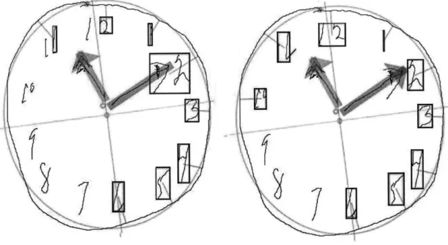
Figure 3.2: Sample One;

In the first sample, neither the old(left) or new(right) algorithm gets all of the numbers correct. However, the new algorithm classifies the 10 correctly where the old method did not find the 10. In addition, the old algorithm found only one digit of both the 11 and the 12. The new algorithm found both digits, because it looked for more strokes when it did not initially find the minimum number expected (in the case of the 11 and the 12, the minimum is 2). Finally, the arrow on the minute hand was classified as part of the 2 in the old algorithm. This mistake was not made with the new algorithm.

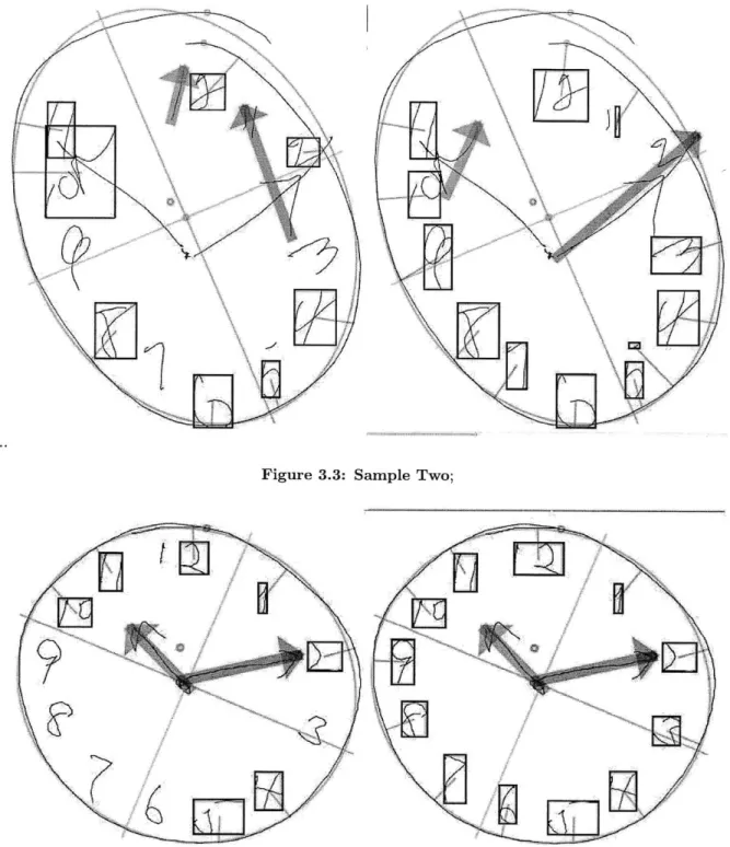
In sample two, the old(left) algorithm classifies only half of the numbers correctly. The new(right) algorithm does much better, missing only 3 of the numbers. The Rotational Classifier was able to recognize the sequence of numbers from 5 to 12, even though the individual numbers are not drawn in the correct locations. The three errors are a result of the 2 being classified as part of the minute hand, because it overlaps with the arrowhead. For this reason, the 3 is classified as the 2, the 4 as the 3, and the top of the 5 is called the 4. The hour hands are not found in either case, but the new algorithm is able to correctly identify the minute hand.

As in the previous samples, the old(left) algorithm does not find all of the numbers on the clock in sample three. However, in this case the new(right) algorithm correctly classifies all of the

(22)

dig-Figure 3.3: Sample Two;

Figure 3.4: Sample Three;

its. Despite the fact that numbers are shifted slightly from their expected angles, the Rotational Classifier can still recognize them because they do not overlap and are drawn clearly.

(23)

7-3.4 Visual to Numerical Transformation

Over all, digit classification is improved tremendously. Administration of the Clock Drawing Test should now only require a few small fixes by doctors, rather than classifying each digit by hand in the worst cases. We now move on to discuss the transformation of this visual data to spreadsheet format.

3.4

Visual to Numerical Transformation

After the elements on the clock face have been classified correctly, as approved by the doctor, the file is saved in a .csk format. The next step is to export the data to an .xls file, which will record all of the clock data in numerical format. The Clocksketch program has the ability to make certain measurements once the digits are all identified, including measures of time, distance, and angle. The doctors and researchers leading the CDT project have decided upon a list of features that should be recorded, agreeing that these features have potential diagnostic value. The data analysis stage will attempt to pick out specific valuable features, but in the data collection stage our goal is to maintain all of the potentially important data without losing any information. The information recorded is divided into 10 categories.

Patient Information

This section contains information identifying the patient. It includes name, facility, medical record number, diagnosis, gender, handedness, and other facts collected from the patient not related to the CDT. Some of these factors, such as gender, may turn out to be critical pieces of information for diagnosis. However, for the most part, this data is mainly used for identification purposes. Drawing

The Drawing category contains only 3 measurements. The first is Drawing Type, which is either "command" or "copy". For each patient, there will be one page of the .xls spreadsheet dedicated to information about the command clock and another to the copy clock. This feature identifies which clock the data represents. The other two features are number of strokes and total time, both measured for the entire clock. Although these are simple measurements, we expect that they are critical to differentiate our healthy patients.

Clockface

This section records all data related to the Clockface stroke, the outer circle of the clock. Measure-ments include number of strokes, total time, and speed. For the speed measurement, the clockface

(24)

is divided up into quartiles and four different speeds are recorded. The goal of this approach is to determine if the patient slows down or speeds up during certain parts of the circle. Other features include measurements of symmetry, horizontal and vertical diameter, and location of the center. "Closedness" measurements indicate whether or not the patient was able to complete the circle, and how close their ending point is to their starting point.

Hands

The next two sections are dedicated to the minute hand and the hour hand. Each records total length, time and number of strokes. In addition, the center of mass is recorded as well as distance from the center of the clock. Direction of drawing is recorded for both the hand and the (potential) arrow on the end of the hand, both of which are either "outward" or "inward." Finally, the angle of the hand is recorded in addition to the difference of this angle from the ideal angle of the hand.

Hand Pairs

The Hand Pairs section contains information about the relationship between the minute hand and the hour hand. Measurements include x and y intersection, as well as the angle between the two hands.

Numbers

There are two parts to the Numbers section- an overall numbers analysis and specific details about each number. The Numbers Analysis section contains average width and height of the digits as well as the number of digits missing. The next section records information such as the number of strokes, total time, and length of each individual digit. The center of mass of each digit is recorded as an x and y coordinate, along with the height and width of the digit. An OutsideClockface feature records if the digit was drawn inside or outside of the Clockface Stroke, because some patients will be unable to place digits correctly. Finally, the absolute angle of the digit, the difference from ideal angle of the given digit, and the distance from the circumference of the circle are recorded. We predict that comparing the placement of specific digits on the face of the clock will be a key factor in differential diagnosis.

Hooklets

Hooklets are abrupt changes in direction at the end of a stroke. When drawing the numbers on a clock, it is a common phenomenon for subjects to leave a "tail" on one digit that points in the direction of the next digit to be drawn. This is because the pen has not been fully lifted off of the

(25)

3.5 The Final Data

paper before the hand moves towards the next digit. An example of a hooklet can be seen in Fig 3.5.

Figure 3.5: Sample Hooklet;

Information such as the length, slope, and speed of each hooklet are recorded, as well as which digit they are part of and the distance to the following digit. It is predicted that the presence of hooklets will indicate a foresight or planning capability in the patient, that of planning the next digit while they are still drawing the current one, that will be absent in patients who have certain mental deficencies.

Non-Standard Symbols

This section contains information about symbols that are only present in some patients' drawings. These include a center dot for the clock, tick marks along the circumference, text that has been written on the page, and any digits over 12 that are written. The presence or absence of certain extra features may be indicative of specific mental deficencies.

Latencies

The final category of features that is recorded for each clock is Latencies, or lag time between different parts of the sketch. Latencies are recorded between different parts of the clock, such as the Clockface and the hands or the hands and the center dot. The inter-digit latency is also recorded, which is the average time that the patient takes between digits. Large latencies indicates a long pause between each part of the drawing, which could be indicative of different mental conditions.

3.5

The Final Data

A third sheet in the .xls file contains a long list of features for the patient. All of these features come directly from the measurements above, and some are derivative of these measurements. For example, this final list has space allotted for 9 hand pairs. If information about only one hand

(26)

pair was recorded above, then the remainder of the entries will be filled with zeroes.

The final list of features was agreed upon in a joint effort between doctors and researchers. The goal is to include all features that could be potentially useful in diagnosis, losing as little information as possible between the sketch and the database. Currently there are 1017 features that are recorded for each clock, making a feature vector of about 2000 for each patient. The next step is to analyze our data and discover which of these features can be used to differentially diagnose neurodegenerative diseases. How do we deal with data so large, and figure out which of these features actually have diagnostic value? This is the question that will be addressed in the next section.

(27)

The Multitool Data Analysis Package

4.1

Introduction

After the data collection stage, we are left with feature vectors approximately 2000 features in length for each patient. These vectors contain spatial and temporal information about both the command clock and the copy clock, as well as other information such as patient gender and age. How do we take this large set of data and find common trends? Is there, for instance, a group of features that take on extreme values in patients with Alzheimer's disease as opposed to patients with Parkinson's?

This problem calls for the use of data mining and machine learning tools such as clustering, di-mensionality reduction, and self-organizing maps. A large number of tools are available today that provide the functionality of machine learning algorithms. However, when the domain of data is relatively new, such as data collected from patients in the CDT, it is difficult to know in advance which of these techniques will be most useful in uncovering trends or patterns. Since each individual tool requires a unique data input format, the conversion can be a tedious process, particularly when data mining is in the exploratory phase.

In order to solve this problem for CDT data analysis, I developed the Multitool Data Analysis (MDA) Package. This tool unifies different approaches to data mining on a single, easy-to-use platform. The MDA Package is designed to provide several options for analysis techniques, to provide file conversion for ease of use, and to facilitate easy launching of the programs from a single interface.

While many excellent tools are available in the machine learning community, each has drawbacks that make exclusive use undesirable. For example, Cluster 3.0, the clustering tool chosen for

(28)

the MDA Package, allows for easy and direct modification of clustering parameters, but has no method for visualization of results. WEKA is probably the most common machine learning tool, as it provides many different functionalities, but it lacks the customization capability that more focused tools provide.

With the ability that the MDA Package provides to easily launch several tools, analysts will be able to more easily determine which techniques are most useful for their domain. One difficulty that arises when trying to use several analysis tools is that each requires its own idiosyncratic in-put file format, and some require additional template or header files. The MDA Package provides functionality that converts data in the well known .csv format into formats usable by each of the six selected tools. Rather than requiring the user to create input files for each program by hand, the package generates the necessary files from a .csv data file.

The MDA Analysis Package currently launches six machine learning tools:

" Weka: A multi-faceted tool providing clustering, dimensionality reduction, and supervised classification tools.

* Cluster 3.0: A tool that allows the user to directly edit parameters in the k-means clustering algorithm, the self-organizing map algorithm, and in principle components analysis. " Databionics ESM: A tool that allows the user to see a 2D visualization of dimensionality

reduction by SOMs.

" BSVM: A tool that trains a support vector machine with a focus on multi-class classification, allowing the user to edit paramaters.

" PCA and EPCA, both for dimensionality reduction.

These six tools were chosen for the collective depth and breadth that they provide to an analyst, and to include tools for both supervised and unsupervised learning methods.

4.2

MDA Package

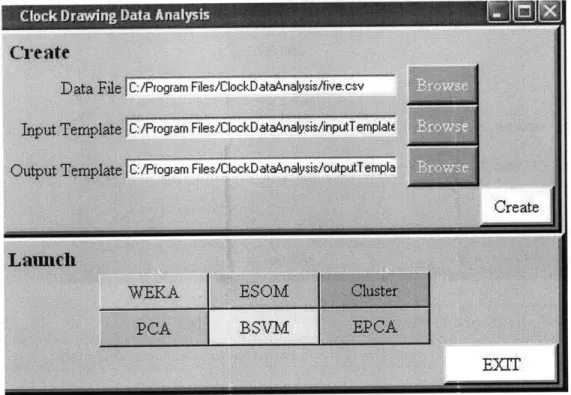
The MDA Analysis Tool can be run either as a command-line application or from a graphical user interface. The graphical interface is customized to work with CDT data, so analysis of other data must be done through the command-line option. The interface is simple to use, with an upper

(29)

4.3 File Creation

Figure 4.1: User Interface for CDT Data;

panel for file creation and a lower panel for launching the six available machine learning tools.

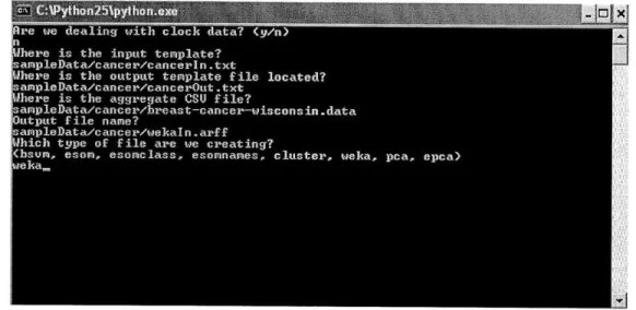
Data that is not derived from the Clock Drawing Test can be formatted for machine learning tools using the command line version of this package. The user will be prompted with a series of questions, asking for the location of all of the input files as well as the machine learning tool that will be used. Files can be created for each program individually, rather than in batch form as with the CDT data. We show a sample use of the command line interface in Figure 4.2.

4.3

File Creation

Three input files are used to guide the transformation of .csv files into a format usable by our selection of machine learning tools. One is the raw data file, and the other two are referred to as template files, which contain information on the type of input data and desired output data. The format for these template files was developed to be as simple as possible for the user, but still contain enough information about the input in order to correctly transform the input .csv file. I chose to use separate input and output template files so that different analyses can be performed on the same input data. By simply changing the output template file, the analyst can decide

(30)

Figure 4.2: Text UI;

which features are included in the output files that will be fed to the machine learning tools. ClockSketch Data Files

The Clocksketch software creates a .csv file in a common format, with the first line containing uniquely named features taken from the clock drawings, followed by two lines of data for each patient.

Here are the first few lines from a sample .csv file.

Type , PtNameF, PtNameL , MedicalRec , DocName , DwgTotStrokes , DwgTotTime

CS, "CIN1875169520" ,"86","","Dana Penney",22,25.38900 CS, "CIN1875169520 ","86", "" ,"Dana Penney",25,25.58200 CS,"CIN1525846837","91", "","Dana Penney",82,158.74800 CS,"CIN1525846837","91","" ,"Dana Penney",30,63.19800

This is a standard .csv format, with values separated by commas and no extra spaces. Missing string data is indicated by "", and missing numerical data is indicated by two commas in sequence.

The first line names seven features, and each name is unique. The next two lines have the same PtNameF and PtNameL features, indicating that the data is from the same patient.

Input Template File

The purpose of the input template file is to specify types for each of the features contained in the .csv file. This file will be used to ensure that the data we are analyzing follows an expected format- the analyst should be made aware of any unexpected values that appear in the data before they cause strange results in the analysis stage. The input template file will contain a list of all of

(31)

4.3 File Creation

the features that are expected in the data file; our current feature vectors for the Clock Drawing Test are about 2000 in length. In addition to the name of each feature, the type of the feature will be included so that type checking can be performed before file creation. Specifications for the input template file can be found in Appendix A.

Here are a few lines from a sample input template file. To keep the example short, ellipses have been used to indicate text that is left out. Further explanation of the example can also be found in Appendix A. Type NA PtNameF NA PtNameL NA MedicalRec NA DocName NA FacilName NA

PtDiagnosisl {ADD,ADHD,Alcohol Related,... .

DwgType NA DwgTotStrokes int

DwgTotTime real

ClockFacelTotStrokes int

ClockFace1TotTime real

Mapping Input to Output

In order to facilitate flexible data analysis, MDA allows the analyst to define the list of output features in the output template file. Some of these output features will be functions of the input features, rather than a direct mapping of the input value to the output file. For example, the analyst might want to look at trends in the time it takes to draw the 1-3, and therefore want to add together digit and latency times.

To accomodate any derived features that the analyst wants to study, the file creation component of MDA contains a section in which "transform functions" can be defined. These functions are written in Python, and therefore some familiarity with Python is required of the analyst. The analyst needs to define any transform functions that are needed to compute new features from those in the .csv file. The transforms.py file holds these functions. Each function takes two lists as input: a list of input features and a list of additional parameters. Here is a sample function, Pure, as seen in the above example of an output template file.

(32)

def Pure(x, args): return x[0]

See Appendix A.2 for transform function specifications and a more complex example of a trans-form function.

Output Template File

The output template file indicates the mapping between data in the .csv file and the desired output data we want to analyze. For example, we may want to look at only a few features of the input data. Or, the features that we want to analyze may be functions of several of the input features. See Appendix A.3 for specifications of the output template file.

Here are the first few lines from a sample output template file.

ClockFacelTotStrokesCOMMAND Pure {ClockFaceTotStrokesCOMMAND} {} int

ClockFacelTotTimeCOMMAND Pure {ClockFacelTotTimeCOMMAND} _{} _real ClockFacelTotLenCOMMAND Pure {ClockFacelTotLenCOMMAND} _{} real ClockFace1PnSpdQ1COMMAND Pure {ClockFace1PnSpdQ1COMMAND} _{} real ClockFacelPnSpdQ2COMMAND Pure {ClockFace1PnSpdQ2COMMAND} _{} real

Names in the first column (the output features) can be chosen by the analyst. The rows in this example each use the Pure function, which means that the value of the feature contained in column three will be passed on to the output. If there aren't any extra parameters for the function, as in this case, column four contains empty brackets. As in the input template file, the final column is used for type-checking on the values that will be printed to the output files. An error message will indicate if any output values are calculated that do not match the expected output value type. It is important for correct file creation that the output feature to be used as the class is the last row in the output file. See Appendix A.3 for another example of an output template file.

Output Specifications

The file creation functionality of MDA will provide a directory of files for use with the six provided machine learning tools. The directory will be named according to the time of its creation, and subdirectories will contain files for each of the tools. These files should be opened with the appropriate tool for further analysis. See Appendix B for an example of the complete process of file creation.

(33)

4.4 Machine Learning Tools

4.4

Machine Learning Tools

The MDA Tool can launch six machine learning tools; this section explores use of these tools using a sample cancer dataset. Four of these tools are stand-alone tools that could be used outside of MDA, while two were developed specifically for the MDA Package. More details on use of each of the tools can be found in Appendix C.

4.4.1 Weka

Weka is a tool that is well known in the machine learning community for the number of algorithm implementations it provides and its easy-to-use interface.

One valuable feature of Weka is its ability to easily preprocess data. Certain features can be selected/deselected, and then removed from the dataset. This functionality is useful if the analyst wants to observe the results of classification based on a subset of the features recorded. A side panel provides a bar graph of the distribution of the samples for each feature selected; for each possible value of the feature, the graph indicates how many of the samples have this feature value. This is useful because it allows the analyst to quickly and easily recognize the distribution across each feature.

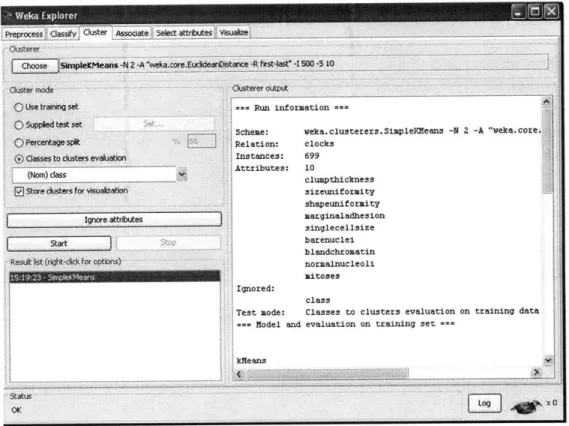
Weka provides both supervised and unsupervised learning functionality. For example, k-means clustering is an unsupervised learning tool and the decision tree algorithm is a supervised classi-fication method, both available in Weka. Once preprocessing is completed, these algorithms can be run and the output will be displayed on the right-hand panel of the interface. The interface is text based, so there is no visualization functionality for algorithms such as clustering or linear separators.

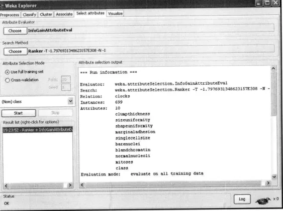
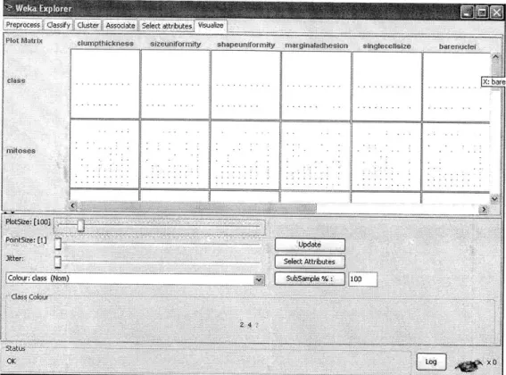
In addition, Weka provides association, attribute selection, and visualization capabilities. The Associate functionality will generate rules that partition the data into classes. The Select At-tributes functionality includes algorithms such as Principles Components Analysis, which reduces the dimensionality of the data by choosing to keep only features that account for high variance in the data. Finally, the Visualization capability shows graphs of pairwise comparisons between features of the data. This is useful for determining if any features are correlated, or just visualizing the relationship between any two features.

Weka provides a wide array of tools for the user to begin analyzing a dataset. More detailed information about Weka, as well as sample usage, is available in Appendix C.1.

(34)

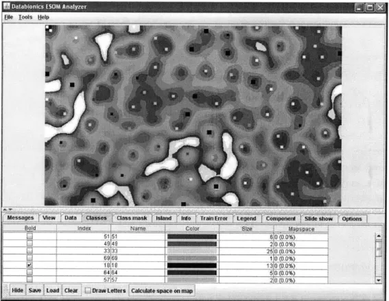
4.4.2 DataBionics ESOM

The ESOM (emergent self-organizing map) tool provided in the MDA Package has a more focused functionality than the WEKA tool. An ESOM is a projection of high-dimensional space onto a two-dimensional "map", with distances in the higher-dimensional space indicated by differing col-ors on the map. The major advantage to using this tool for data analysis is that it provides a detailed map of the data and a visual representation of any clustering that occurs in the data. The program requires the user to load three files, all of which are provided by the file creation functionality of the MDA Tool. (Appendix C.2)

4.4.3 Cluster 3.0

The clustering tool provided in the MDA Package was originally developed for clustering of DNA microarray data, and therefore has the capabilities required to handle large datasets. Although Cluster 3.0 contains PCA and SOM functionality, better implementations of these algorithms can be found in the PCA and ESOM tools. However, the clustering functionality of Cluster 3.0 allows for tight control over parameters by the analyst. Data can be centered and normalized before clustering is performed, and eight different distance metrics can be chose for the k-means clustering algorithm. The number of clusters and iterations of the algorithm must also be chosen before run time. Clustering output is a text file which contains a list of each of the samples in the data and the cluster to which they have been assigned. (Appendix C.3)

4.4.4 BSVM

The BSVM tool provided is a tool for training SVMS on the data, allowing users to select desired kernel type, loss function, tolerance, and many other parameters. BSVM allows the user to choose from four different algorithms for multi class classification: bound-constrained multi-class support vector classification (SVC), class SVC from solving a bound-constrained problem, multi-class SVC from Crammer and Singer, and bound-constrained support vector regression. Users can edit type of SVM, kernel type, and values for 12 other parameters. Once a model has been trained, it can be used to classify new unlabeled data. (Appendix C.4)

4.4.5 PCA

The PCA tool provided performs principle components analysis on the data and returns a new dataset in which the number of features has been reduced. Researchers