Bayesian Variable Selection in High Dimensional Genomic Studies Using Nonlocal Priors

(1)

BAYESIAN VARIABLE SELECTION IN HIGH DIMENSIONAL GENOMIC STUDIES USING NONLOCAL PRIORS

A Dissertation by

AMIR NIKOOIENEJAD

Submitted to the Office of Graduate and Professional Studies of Texas A&M University

in partial fulfillment of the requirements for the degree of DOCTOR OF PHILOSOPHY

Chair of Committee, Valen E. Johnson Committee Members, Wenyi Wang

Anirban Bhattacharya Natarajan Sivakumar Head of Department, Valen E. Johnson

December 2017

Major Subject: Statistics

(2)

ABSTRACT

The advent of new genomic technologies has resulted in production of massive data sets. The outcomes in such experiments are often binary vectors or survival times, and the covariates are gene expressions obtained from thousands of genes under study. Analysis of these data, especially gene selection for a specific outcome, requires new statistical and computational methods. In this dissertation, I address this problem and propose one such method that is shown to be advantageous in selecting explanatory variables for prediction of binary responses and survival times. I adopt a Bayesian approach that utilizes a mixture of nonlocal prior densities and point masses on the regression coefficient vectors. The proposed method provides improved performance in identifying true models and reducing estimation and prediction error rates in a number of simulation studies for both binary and survival outcomes.

I also describe a computational algorithm that can be used to implement the methodol-ogy in ultrahigh-dimensional settings (p≫n). In particular, for survival response datasets I show that MCMC is not feasible and instead provide a computational algorithm based on a stochastic search algorithm that is scalable andpinvariant.

As part of the variable selection methodology, I also propose a novel approach for setting prior hyperparameters by examining the total variation distance between the prior distributions on the regression parameters and the distribution of the maximum likelihood estimator under the null distribution. An R package, BVSNLP, is also introduced in this dissertation as a final product which contains all described methodology here. It performs high dimensional Bayesian variable selection for binary and survival outcome datasets that is expected to have a variety of applications including cancer genomic studies.

(3)

extending Uniformly Most Powerful Bayesian tests (UMPBTs) from exponential fam-ily distributions to a larger class of testing contexts. UMPBTs are an objective class of Bayesian hypothesis tests that can be considered the Bayesian counterpart of classical uni-formly most powerful tests. However, they have previously been exposed for application in one parameter exponential family models. I introduce sufficient conditions for the ex-istence of UMPBTs and propose a unified approach for their derivation. An important application of my methodology is the extension of UMPBTs to testing whether the non-centrality parameter of aχ2 distribution is zero.

(4)

DEDICATION

To my darlingBornaand belovedArezou

(5)

ACKNOWLEDGMENTS

I would like to express my deepest gratitude towards my advisor and mentor forever, Dr. Valen E. Johnson for his generous support throughout my doctoral studies. He was always there when needed, regardless of the type of my hardship. Ethics, manners and style of research are his main attributes I admire the most and will remember forever. Thank you Val, you have been a great inspiration to me and a perfect role model for my professional career.

I thank all the members of my dissertation committee, especially Dr. Wenyi Wang. She acquainted me with the marvelous world of cancer genomics and accepted me as one of her group members in MD Anderson Cancer Center, in the first year of my Ph.D. studies. Thanks also to Dr. Michael Longnecker for his all time support for the graduate students in the department and giving me the opportunity to teach an undergraduate course for two semesters.

I am obliged to the Texas A&M High Performance Research Computing (HPRC) and their staff for providing a powerful cluster which facilitated the simulation and real data analyses of my dissertation. Without them, it was impossible to accomplish my doctoral research objectives.

Special thanks to the kind, friendly and responsible staff of the statistics department. Sandra, Athena, Deanna, Elaine and Andrea, I appreciate your help in guiding me dealing with other necessary aspects of graduate student life besides academic research.

While studying in College Station, I was fortunate enough to be around very wonderful and kindhearted friends who were like family far from the family. Friends who were supportive through highs and lows and were always there to hangout with on weekends when shaking off stress from an onerous week seemed vital. Mehdi, Somayeh, Mohsen,

(6)

Hoda, Zoya and Peyman, without you this journey would not be as invigorating and joyful. Thank you!

I am deeply indebted to my family. First and foremost, my parents and my parents-in-law for their unflinching support from thousands miles away, and then my sisters Nastaran and Yasaman and my brother-in-law, Payam. Their encouragement, in all possible ways, has always bolstered my confidence and helped me advancing through my graduate studies here in the US.

Last but not the least, I want to dedicate this work to my life companion and the love of my life, Arezou. She was the one who saw the potential in me and helped me succeed in what seemed infeasible at the beginning: withdrawing from Ph.D. of electrical engineering after two years and re-applying to the Ph.D. of statistics. That turned out to be one of the best decisions I have made in my life. I would never forget her support and encouragement through hard days of my doctoral studies. My dear, without you none of this would have been possible and you are always my courage in my academic quest.

(7)

CONTRIBUTORS AND FUNDING SOURCES

Contributors

This work was supported by a dissertation committee consisting of Professor Valen E. Johnson, Dr. Wenyi Wang and Dr. Anirban Bhattacharya of the Department of statistics and Dr. Natarajan Sivakumar of the Department of mathematics.

Parts of the cancer genomic data analyzed in Chapter 3 and 4 were provided by Dr. Wenyi Wang and her group in the department of Bioinformatics and Computational Biol-ogy in University of Texas MD Anderson Cancer Center.

All other work conducted for the dissertation was completed by the student indepen-dently.

Funding Sources

Graduate study was supported by Graduate Assistant Teaching (GAT) and Graduate Assistant Non-Teaching (GANT) funds from the department of statistics at Texas A&M University, in addition to Graduate Assistant Research (GAR) funding from National Insti-tute of Health grant (R01CA158113) and National Cancer InstiInsti-tute grant (1R01CA174206-01).

(8)

NOMENCLATURE

AUC Area Under Curve

BMA Bayesian Model Averaging

BVS Bayesian Variable Selection

CRAN Comprehensive R Archive Network

GLM Generalized Linear Models

HPPM Highest Posterior Probability Model

HFM Highest Frequency Model

iMOM Inverse Moment Prior

ISIS Iterative Sure Independence Screening

MCMC Monte Carlo Markov Chain

MOM Moment Prior

MPI Message Passing Interface

MPM Median Probability Model

NLP Nonlocal Prior

pMOM Product Moment Prior

piMOM Product Inverse Moment Prior

ROC Receiver Operating Characteristic

TCGA The Cancer Genome Atlas

(9)

TABLE OF CONTENTS

Page

ABSTRACT . . . ii

DEDICATION . . . iv

ACKNOWLEDGMENTS . . . v

CONTRIBUTORS AND FUNDING SOURCES . . . vii

NOMENCLATURE . . . viii

TABLE OF CONTENTS . . . ix

LIST OF FIGURES . . . xii

LIST OF TABLES. . . xiii

1. INTRODUCTION. . . 1

1.1 Motivation and Background . . . 1

1.2 Main Contribution to the Problem . . . 5

2. BAYESIAN HIERARCHICAL MODELS, NONLOCAL PRIORS AND HY-PERPARAMETER SELECTION . . . 8

2.1 Introduction . . . 8

2.2 Moment and Inverse Moment Nonlocal Priors . . . 9

2.3 Hierarchical Bayesian Modeling in Variable Selection . . . 12

2.3.1 Laplace Approximation to Marginal Probabilities . . . 14

2.3.2 Prior on Model Space . . . 16

2.4 Hyperparameter Selection . . . 17

2.4.1 Justification For1/√pOverlap. . . 20

2.5 Discussion . . . 22

3. HIGH DIMENSIONAL BAYESIAN VARIABLE SELECTION FOR BINARY RESPONSE DATA . . . 23

(10)

3.2.1 Nonlocal Priors . . . 26

3.2.2 Prior on Model Space . . . 27

3.2.2.1 Choosing Hyperparameters . . . 28

3.3 Numerical Aspects of Implementation . . . 29

3.3.1 Convergence Diagnostics . . . 30

3.4 Results . . . 31

3.4.1 Simulation Studies . . . 32

3.4.1.1 Sensitivity Analysis for Prior Parameters on Model Space 35 3.4.2 Real Data Analysis . . . 36

3.4.2.1 Leukemia Data . . . 38

3.4.2.2 Renal Cell Carcinoma Data . . . 39

4. HIGH DIMENSIONAL BAYESIAN VARIABLE SELECTION FOR SURVIVAL DATA . . . 43

4.2 Methods . . . 45

4.2.1 Preliminaries . . . 45

4.2.2 Product Inverse MOMent (piMOM) Prior . . . 47

4.2.3 Highest Posterior Probability Model . . . 50

4.2.3.1 Calculating the Gradient and Hessian ofg(βk). . . 51

4.2.3.2 Stochastic Search Algorithm . . . 53

4.3 Results . . . 55

4.3.1 Simulation Studies . . . 55

4.3.2 Real Data . . . 58

4.3.2.1 Leukemia Data . . . 58

4.3.2.2 Renal Cell Carcinoma Data . . . 60

5. ON EXISTENCE AND DERIVATION OF UNIFORMLY MOST POWERFUL BAYESIAN TESTS WITH APPLICATION TO NON-CENTRALχ2 _{TESTS . . .} ₆₂

5.2 Method . . . 64

5.2.1 Preliminaries . . . 64

5.2.2 Existence and Derivation of UMPBT . . . 65

5.3 UMPBTs for Common Tests of Hypotheses . . . 68

5.3.1 UMPBT for Chi-squared Tests . . . 69

5.3.2 Exponential Family Distributions . . . 70

5.4 Results . . . 72

5.4.1 Analysis of Evidence Threshold. . . 72

(11)

6. BVSNLP: THE R PACKAGE FOR HIGH DIMENSIONAL BAYESIAN VARI-ABLE SELECTION . . . 77

6.2 General Points of BVSNLP Package . . . 78

6.3 Details of Important Functions . . . 79

6.3.1 PreProcess() Function. . . 79

6.3.1.1 Description of Input Arguments . . . 79

6.3.1.2 Description of Output Arguments. . . 80

6.3.2 HyperSelect() Function . . . 80

6.3.3 bvs() Function . . . 81

6.3.4 ModProb() Function . . . 89

6.3.5 CoefEst() Function . . . 90

6.3.6 predBMA() Function. . . 91

7. CONCLUSIONS . . . 95

(12)

LIST OF FIGURES

FIGURE Page

2.1 pMOM prior with r = 1andτ = 0.8and piMOM prior with r = 2and τ = 0.8. . . 11 2.2 Example of overlap between a piMOM prior and approximate normal

dis-tribution of null MLE coefficients. . . 18 3.1 piMOM prior forr = 1.5andτ = 1. . . 27 3.2 Average true and false positive counts for all 30 different simulation settings. 34 3.3 10-fold cross validation MSE( ˆπ)of iMOMLogit vs. ISIS-SCAD, forp=

1000andp= 10,000. . . 36 3.4 Sensitivity analysis for parameters of prior on model space. . . 37 4.1 Average AUC of both BVSNLP and CoxHD methods after 5 fold cross

validation for AML dataset. . . 59 4.2 Average AUC of BVSNLP method after 5 fold cross validation for renal

cell carcinoma dataset. . . 61 5.1 Relation between increasing or decreasing nature of the Bayes factor and

the type of boundedness inΩγ(θ1). . . 68 5.2 Evidence threshold vs. degrees of freedom in Chi-squared tests for

(13)

LIST OF TABLES

TABLE Page

3.1 Selectedτ parameter of piMOM prior for different simulation settings . . . 33 3.2 Selectedrparameter of piMOM prior for different simulation settings . . . 33 3.3 Comparison between iMOMLogit and other methods for leukemia data set 39 3.4 Comparison between iMOMLogit and other methods for renal cell

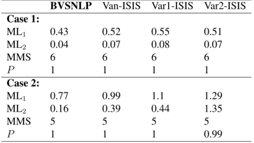
carci-noma data set . . . 41 4.1 Comparison between BVSNLP and ISIS-SCAD for simulation cases 1 and

2. n = 400andp= 1000. . . 57 5.1 White and Eisenberg (1959) classification of cancer patients . . . 74 5.2 Bayes factors based onχ2_{-statistic and UMPBT}₍_γ₎_{non-centrality}

(14)

1. INTRODUCTION

1.1 Motivation and Background

The emergence of mircoarray data in late 1990’s and the advent of high throughput gene sequencing technology in mid 2000’s introduced a new era which led to the produc-tion of numerous ultrahigh dimensional gene expression datasets. The Cancer Genome Atlas (TCGA) and International Cancer Genome Consortium (ICGC) are generating large amounts of high dimensional genomic data making those data available to the research community. These data are generated from myriad studies performed by independent researchers and include DNA copy-number alterations (CNA), mRNA and microRNA ex-pressions and other types of gene-related explanatory variables. An online portal named cBioPortal (Gao et al., 2013) facilitates accessing these datasets via an intuitive Web in-terface where researchers and clinicians can do various analysis as well as downloading desired data.

This revolution has prompted a new direction in statistical data analysis as well as biomedical and bioinformatics research. Traditional statistical methods cannot be applied to datasets with small samples and very large numbers of covariates. This topic has in-spired various statisticians from both frequentist and Bayesian schools of thought and resulted in development of new methodologies. The goal of variable selection in high di-mensional data is to identify small subset of covariates that are associated with an outcome. This, imposes a sparsity assumption on the problem. In the context of cancer genomics, the target is to determine genes that are associated with the response vector, which can be continuous, binary or a survival time. Interested readers can refer to Guyon and Elisseeff (2003) for more discussion on objectives of variable selection and its related problems.

(15)

A general model for variable selection may be posed as follows,

E(yn) = F(Xβ), (1.1)

whereynis the response vector,Xisn×pdesign matrix andβisp×1coefficient vector. In ultrahigh dimensional settingsp≫n. Depending on values of response vectoryn, this modeling framework encompasses linear regression, logistic regression and other types of generalized linear models. The sparsity assumption implies that the majority of elements inβ are zero, and thus the sparse selection problem is basically identifying the non-zero elements inβ.

A number of methods have been proposed to address this problem. These include the LASSO (Tibshirani, 1996), a penalized likelihood method that maximizes a product of the likelihood function and a constraint on the sum of the absolute value of components of the regression coefficientβ. A closely related method called Smoothly Clipped Absolute Deviation (SCAD) (Fan and Li, 2001) uses a non-convex penalty function and has been demonstrated to have certain oracle properties in idealized asymptotic settings. Other penalized likelihood functions include the adaptive LASSO (Zou, 2006) and the Dantzig selector (Candes and Tao, 2007). These methods share asymptotic properties similar to SCAD. Correspondingly, Efron et al. (2004) proposed Least Angle Regression (LARS), a variable selection method which is a less greedy version of forward selection methods.

In ultrahigh dimensions (p≫n), an effective computational technique for implement-ing the techniques described above is the Iterative Sure Independence Screenimplement-ing (ISIS) procedure (Fan and Lv, 2008), which iteratively performs a correlation screening step to reduce the number of explanatory variables so that penalized likelihood methods can be applied. ISIS has been used in conjunction with several penalized likelihood methods— including adaptive LASSO (Zou, 2006), the Dantzig Selector (Candes and Tao, 2007),

(16)

and SCAD (Fan and Li, 2001)—to perform model selection. Elastic net (Zou and Hastie, 2005) can also be included in the list of variable selection methods suited for ultrahigh dimensional datasets.

Besides penalized likelihood methods, Guyon et al. (2002) proposed an algorithm by exploiting support vector machine methods based on recursive feature elimination. Wang et al. (2005) take a combination of machine learning algorithms such as decision trees and with a correlation based feature selector to perform gene selection.

A number of Bayesian methods have also been proposed for variable selection by specifying a prior distribution onβ vector. Notable among these are the approaches pro-posed by George and McCulloch (1997), which used a mixture-of-normals approximation to spike-and-slab priors on the regression coefficients. Rossell et al. (2013) and Johnson and Rossell (2012) also exploit the two component mixture prior where nonlocal priors are used for non-zero components of the coefficient vector. Rossell et al. (2013) address the problem of identifying variables with high predictive power. Along similar lines, Shin et al. (2015) utilized nonlocal priors for linear regression and showed under some regular-ity conditions the model selection procedure is consistent whenlog(p) =O(nα₎_{. Lee et al.} (2003) proposed a hierarchical probit model along with MCMC based stochastic search to perform gene selection in high dimensional settings using a latent response variable and Gaussian priors on model coefficients. West et al. (2000) provided a Bayesian approach to this problem employing singular value regression and classes of informative prior distribu-tions to estimate coefficients in high dimensional settings. Liang et al. (2008) studied mix-tures ofgpriors for Bayesian variable selection as an alternative to defaultgpriors to over-come several consistency issues associated with the defaultg prior densities. Hans (2009) proposed Bayesian LASSO where the prediction of future observations is also discussed via the posterior predictive distribution. For other significant priors for model coefficients for variable selection, one can refer to Bae and Mallick (2004) for Normal, Laplace and

(17)

Jefferey’s prior, Carvalho et al. (2010) for horseshoe prior and Bhattacharya et al. (2015) for Dirichlet-Laplace prior. Cawley and Talbot (2006) utilized non-informative Jeffery’s prior along with an improved algorithm named BLogReg classification to reduce compu-tational cost in logistic regression gene selection problem.

The aforementioned methods considered variable selection problem in either linear re-gression or generalized linear models. For variable selection models for survival times, many of common penalized likelihood methods originally introduced for linear regression have been extended to survival data as well. These include Tibshirani et al. (1997) where the LASSO penalty is imposed on the coefficients in survival analysis, similar to the linear regression problem. Zhang and Lu (2007) utilized adaptive LASSO methodology for time to event data while Antoniadis et al. (2010) adopted the Dantzig selector for survival out-come. The extension of non-convex penalized likelihood approaches, in particular SCAD, to the Cox proportional hazard model is discussed in Fan and Li (2002). The ISIS ap-proach is also extended for ultrahigh dimensional survival data in Fan et al. (2010) where it is used on Cox proportional hazard models and the SCAD penalty is employed for vari-able selection.

Some Bayesian approaches have also been proposed to address this problem. Faraggi and Simon (1998) proposed a method based on approximating the posterior distribution of the parameters in the proportional hazard model where they define a Gaussian prior on a vector of coefficients. A loss function is then defined in order to select a parsimonious model. A semi-parametric Bayesian approach is utilized by Ibrahim et al. (1999), where they employ a discrete gamma process for the baseline hazard function and a multivariate Gaussian prior for the coefficient vector. Sha et al. (2006) considered Accelerated Failure Time (AFT) models along with data augmentation to impute censored times. A mixture prior in a similar fashion to George and McCulloch (1997) is exploited for sparse selection procedure.

(18)

Due to the huge computational load of Bayesian data analysis imposed by Monte Carlo Markov Chain (MCMC) procedure, in particular for high dimensional survival data, the frequentist approaches outnumber their Bayesian counterparts in real genomic applica-tions. Consequently, developing a fairly fast Bayesian variable selection method for high dimensional datasets that can outperform dominant frequentist algorithms seems com-pelling.

1.2 Main Contribution to the Problem

As described in the previous section, it is encouraging to develop a fast and precise Bayesian variable selector to be applied to various datasets. In this dissertation, I propose a Bayesian hierarchical model where I use a mixture of point mass probabilities and nonlocal priors for vectors of coefficients. The targets of my methodology are cases when the response vector is binary or a survival time. For the former, a logistic regression model is used while for the latter, I utilize Cox proportional hazard models (Cox, 1972). A key feature of my methodology is the automatic selection of hyperparameters of nonlocal priors. In addition, I adopt the stochastic search algorithm with screening introduced by Shin et al. (2015) for survival data in order to make the algorithm scalable and hence invariant to the number of covariates,p.

By testing my algorithm in various simulation datasets under different settings of sam-ple size, number of covariates and correlation matrices, I found the output results were more precise (less false positives in selected variables) and had smaller coefficient esti-mation error rates in comparison with existing methods. I also applied my algorithm to different important cancer genomics datasets under both binary and survival time scenar-ios. Those include the Golub leukemia data (Golub et al., 1999), renal cell carcinoma (Cancer Genome Atlas Research Network, 2013) and the AML leukemia dataset intro-duced in Papaemmanuil et al. (2016). In all cases, my method picked sparser models with

(19)

better predictive accuracy.

Another contribution of this dissertation is the development of an R package named BVSNLP to implement the proposed models and make them accessible to researchers. Within each iteration of the algorithm, various nonlinear optimization procedures, as well as Laplace approximation to approximate marginal probability of the data, are performed. These calculations incur immense computational burden. As a result, I implement the models in C++ in order to speed up the computation. Parallel computing ability is an-other feature of the BVSNLP package. Coupling algorithm in logistic regression variable selection as well as parallel stochastic search algorithm in survival variable selection are algorithms in the package that are benefited from this feature. These are discussed in detail in the forthcoming chapters.

In addition to variable selection, I also studied Uniformly Most Powerful Bayesian Tests, UMPBTs, to extend the work by Johnson (2013c) to a more general class of sam-pling distributions by providing a sufficient condition for the existence of such tests, as well as a general approach to derive them. The primary application for this extended work is in testing the non-centrality parameter inχ2 _{statistics with arbitrary degrees of freedom} being equal to zero. This is largely used in contingency tables, χ2 _{tests, likelihood ratio} tests or even model selection procedures (Hu and Johnson, 2009).

The following chapters are organized as follows. In Chapter 2 I discuss the preliminar-ies which include Bayesian hierarchical models, a brief review on nonlocal prior densitpreliminar-ies, the proposed algorithm for hyperparameter selection and the general scheme of Bayesian model selection procedures. Chapter 3 explains my method for binary response data in detail with simulation and real data results. Chapter 4 extends the methodology to datasets with survival time outcomes. The research reported for binary response vectors in Chap-ter 3 has been published in Bioinformatics(Nikooienejad et al., 2016). The extension to UMPBTs and its existence conditions are discussed in Chapter 5, where some examples

(20)

of its application to contingency tables are provided. The aforementioned R package is introduced in Chapter 6 where each of its important functions are investigated in detail. Concluding remarks appear in Chapter 7.

(21)

2. BAYESIAN HIERARCHICAL MODELS, NONLOCAL PRIORS AND HYPERPARAMETER SELECTION∗

2.1 Introduction

High dimensional variable selection problems were introduced in Chapter 1, and a re-view of common approaches that have been proposed in the past ten to fifteen years was also provided. The main assumption in such problems is sparsity of the vector of coeffi-cients. Sparsity soluion are achieved by penalizing the likelihood function in frequentist approaches. In Bayesian methods, sparsity is imposed by the prior distribution defined on the coefficients, in conjunction with the prior on the model size. In this dissertation, a hier-archical mixture model is constructed in whichπ(yn|β)denotes the likelihood function, π(β) denotes the prior on the coefficients and π(k) denotes the probability of model k, which depends only on model size. The choices for π(β), p(k)and the numerical proce-dure that computes the posterior probabilities are the main characteristics of any Bayesian approach to perform variable selection.

A list of notable sparsity priors proposed for β can be categorized into the follow-ing. Discrete mixture priors (Johnson and Rossell, 2012; George and McCulloch, 1997), Student t distributions (Tipping, 2001), horseshoe priors (Carvalho et al., 2010), Nor-mal/Jefferey’s priors (Bae and Mallick, 2004), Normal/exponential-gamma priors (Griffin et al., 2010), and double exponential densities (West, 1987; Park and Casella, 2008; Peric-chi and Smith, 1992; Hans, 2009). For more details consult Polson and Scott (2010).

In this dissertation I use the discrete mixture prior structure that defines a point mass at zero for zero coefficients and a nonlocal continuous distribution for non-zero coefficients. ∗_{Part of this chapter is reprinted with permission of Oxford University Press, from the article:}

Nikooienejad, A., W. Wang, and V. E. Johnson (2016). Bayesian variable selection for binary outcomes in high-dimensional genomic studies using non-local priors.Bioinformatics 32(9), 1338-1345.

(22)

In particular, I extend the methodology discussed in Johnson and Rossell (2012) for gen-eralized linear models and Cox proportional hazard models to perform variable selection in high dimensional datasets. The fundamental characteristic of this method is the use of nonlocal priors (Johnson and Rossell, 2010).

In contrast to local priors, nonlocal priors are density functions that are equal to zero at the null value of the random variable. The variable selection problem can be converted to a series of hypothesis tests for coefficients being equal to0, the null value. As discussed in Johnson and Rossell (2010), where local priors are used, the accumulation of evidence in favor of the true null is not at the same rate as that when the alternative is true. Accordingly, for discrete mixture models, the choice of a prior distribution with that characteristics is expected to improve the overall variable selection outcome. For instance in the context of linear regression, Shin et al. (2015) showed that under certain regularity conditions the selection procedure with nonlocal priors is consistent even when the number of covariates p increases sub-exponentially with the sample sizen. Using local prior models leads to the assignment of probability0to the true model.

This chapter is organized as follows. In Section 2.2 I review two of the common nonlocal priors used in variable selection. Section 2.3 describes the hierarchical model used in Bayesian variable selection. In Section 2.4 I propose a data-specific algorithm for automatic selection of hyperparameters for nonlocal priors and Section 2.5 concludes the chapter.

2.2 Moment and Inverse Moment Nonlocal Priors

The two nonlocal priors proposed in Johnson and Rossell (2010) are the moment prior (MOM) and the inverse moment prior (iMOM) prior densities. A base distribution is needed to construct moment priors. The choice of this base prior depends on the tail behavior of the parameter under study. One common choice for the base prior is the

(23)

standard normal distribution. On the other hand, inverse moment priors have functional forms that are related to the inverse gamma density function. In particular, their behavior near the null value is similar to the behavior of inverse gamma distributions near0.

The choice of multivariate MOM or iMOM priors for the vector of coefficients seems a natural choice. However, as shown in Johnson and Rossell (2010), the multivariate form of those priors are0only when all of the components of the vector are zero. This property does not provide a sufficient penalty for models with coefficient estimates near zero. As a result, the product version of such priors, named pMOM and piMOM, are preferred since hey are zero wheneveranyof the components of the regression vector are equal to zero, and get very small when most of the parameter estimates are close to zero.

The pMOM prior with a normal base density for a vector of sizek is defined as π(β|τ, σ2, r) =dk(2π)−k/2(τ σ2)−rk−k/2|Ak|1/2 ×exp [ − 1 2τ σ2β ′_A kβ ]∏k i=1 β2r_i , (2.1)

where τ > 0 and r is a positive integer called the order of the density. Ak is a k ×k nonsingular scale matrix. The normalizing constant dk is independent ofσ2 and τ. The parameterσ2 _{is the variance of the base Gaussian density and is usually assumed to be}₁_.

The piMOM density for a vector of sizek, a product of iMOM density functions, is defined as π(βk|τ, r) = τrk/2 Γ(r/2)k k ∏ i=1 |βi|−(r+1)exp ( − τ β2 i ) . (2.2)

Here,τ is a scale parameter controlling the dispersion of the prior around zero andracts similar to the shape parameter in the inverse Gamma distribution and is responsible for the tail behavior of the distribution. As a result, the roles ofτ andr are critical in the overall

(24)

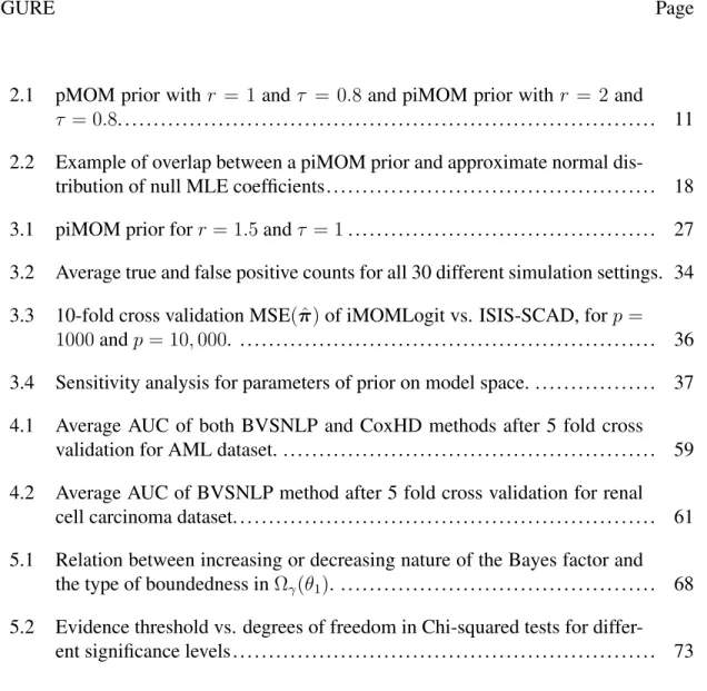
−4 −2 0 2 4 0.0 0.1 0.2 0.3 0.4 0.5 0.6 β Density MOM iMOM MOM iMOM

Figure 2.1: pMOM prior with r = 1 and τ = 0.8 and piMOM prior with r = 2 and τ = 0.8.

performance of the variable selection procedure.

Figure 2.1 depicts an example of both pMOM and piMOM distributions with k = 1. For the plots in this figure, the pMOM parameters arer = 1 andτ = 0.8. The piMOM has parametersr= 2andτ = 0.8.

As illustrated in Figure 2.1, pMOM’s tails are converging to zero at an exponential rate in the same fashion as the Gaussian distribution, while the piMOM’s tails are heavier and are therefore more suitable for capturing larger coefficients. Another important point in comparison of these two densities is their behavior in the vicinity of zero. For the piMOM the region where the prior is close to zero is larger that for the pMOM. This region is controlled by theτ parameter in the piMOM density. The larger τ, the wider that region becomes. As mentioned before, the value of τ is crucial in the selection procedure to penalize covariates with very small coefficient estimates and thus reduce the false positive rate. As a result, the piMOM prior is preferred for the applications discussed here.

(25)

An important feature of the piMOM nonlocal prior, as highlighted in Johnson and Rossell (2012), is that these priors do not necessarily impose significant penalties on non-sparse models provided that the estimated coefficients in the non-non-sparse models are not too small. That is, large values of regression coefficients are not penalized since the value of the exponential kernel in (2.2) tends to 1 as βi becomes large. This fact lies in stark contrast to most penalized likelihood methods. The penalty provided by this prior is on very small coefficient values which makes it a good choice for model selection. It prevents covariates with negligible coefficient estimates from entering the model.

To see how different values ofr andτ change the shape of both pMOM and piMOM priors, refer tohttps://amirnik.shinyapps.io/nlpinteractive/. This webpage provides an in-teractive graphical interface to visualize the effects of hyperparameters on the two afore-mentioned nonlocal densities. Each plotted graph can be downloaded for future purposes as well.

2.3 Hierarchical Bayesian Modeling in Variable Selection

Let the response vector in my analysis beyn which has sizen, the number of obser-vations. It can be a response vector from a linear regression model, a binary vector from a logistic regression model or survival times in a Cox proportional hazard model. In this dissertation, I consider the last two models. Note that all these models involve a coefficient vector,β, where only few number of its elements have non-zero values. Assuming one of the nonlocal priors discussed before is used as the prior for the coefficients, the following hierarchical model can be defined.

(26)

yn|βk∼π(yn|βk,X) : Likelihood function under modelk. βk∼π(βk) : Nonlocal prior on the coefficients.

p(k) : The probability of modelk,

(2.3)

whereXdenotes then×pdesign matrix andβkis the vector of coefficients under model k.

The selection procedure is based on the posterior probability of each model and the model with the highest posterior probability is selected. The posterior probability of model

jis defined as p(j|yn) = p(j)mj(yn) ∑ k∈J p(k)mk(yn) , (2.4)

where mk(yn) denotes the marginal probability of the response vector under model k. The denominator is the normalizing constant that is canceled out when comparing model posteriors. Based on the proposed hierarchical model, the marginal probability of the observed data can be expressed as

mk(yn) =

∫

π(yn|βk)π(βk)dβk. (2.5)

Usually, this integral cannot be calculated analytically and must be numerically ap-proximated. A common method to approximate the integral is the Laplace approximation (Tierney and Kadane, 1986). It is an efficient method because it involves no iteration and avoids numerical integration. A brief review on the first order Laplace method to approxi-mate the marginal probability of data is discussed in the following.

(27)

2.3.1 Laplace Approximation to Marginal Probabilities

The basic idea for Laplace approximation is to approximate the integral

I(t) =

∫

e−th(x)dx, (2.6)

where the goal is to find the value ofI(t)asttends to an asymptotic limit, namely infinity. In this structure, the one dimensional functionh(x)is assumed to have a minimum atx.ˆ

In statistical problems the parameter in asymptotic analysis is usually the sample size, n, which replaces t in the original formulation. Doing a Taylor series expansion of the functionh(x)at its minimum, x, and some integral calculations, the integral in (2.6) canˆ

be rewritten as I(n)≈e−nh(ˆx)(2π n )1/2_ˆ h−₂1 ( 1− ˆ h4hˆ−24 8n + 5ˆh2 3ˆh− 6 2 24n ) . (2.7)

Here, ˆhi denotes the ith derivative of h(x) computed at x. The neglected terms in theˆ expansion above are of the orderO(n−2). As a result, the first order Laplace approximation with a precision to the order ofO(n−1)is computed as

I(n)≈e−nh(ˆx)(2π n

)1/2_ˆ

h−₂1. (2.8)

It can be shown that in the case of multivariate integrals where the variable of integra-tionxisddimensional, the Laplace approximation in (2.8) can be expressed as

∫

e−nh(x)dx≈e−nh(ˆx)(2π)d/2|Σ|1/2n−d/2. (2.9) Here, h(x)is assumed to have a local minimum and |Σ|is the determinant of thed×d matrixΣ, which is equal to the inverse of the Hessian of the function h(x), computed at

(28)

its extreme point,xˆ. That is Σ = H_x_ˆ−1 = [ ∂2h(x) ∂x∂xT ]−1 x=ˆx . (2.10)

To exploit Laplace approximation to approximate marginal probability of data in (2.5), define the functiong(βk)as the negative of the log posterior function:

g(βk) =−log ( π(yn|βk) ) −log(π(βk) ) , (2.11)

and leth(βk) = _n1g(βk). It is then obvious thatmk(yn) =

∫

e−nh(βk)_d_β

k. In addition, let

Gand H denote the Hessian of the functionsg andh, respectively. The determinants of those matrices will then have the following relation

|G|=n−d|H|. (2.12)

By plugging these results into (2.9) and using (2.10), the marginal probability of the response vector under modelkis approximated by

mk(yn) =π(yn|βkˆ )π( ˆβk)(2π)d/2|G_βˆ_k|−1/2. (2.13)

Here,|G_βˆ

k|is the determinant of the Hessian of functiong(βk)computed at

ˆ

βk. Note that

the approximation formula does not directly depend on the sample sizen.

The βˆk is the maximum a posteriori (MAP) estimate of the model which minimizes

the function g(βk) as defined in (2.11). Moreover, if such a point exists for h(βk), the

Hessian is positive definite and consequently all of its eigenvalues are positive. As a result, the determinant ofΣwill be positive.

(29)

review of such methods available in R, refer to Mullen (2014). The main algorithm I use is limited memory version of the Broyden-Fletcher-Goldfarb-Shanno algorithm (L-BFGS) method for large scale optimization (Liu and Nocedal, 1989) that is implemented as a C++ class (Qiu et al., 2016).

2.3.2 Prior on Model Space

Inclusion of covariates in modelkcan be modeled as an exchangeable Bernoulli trials. Let γk = {γ1,· · · , γp} be the binary vector showing which covariates are included in modelk. The size of the model is the number of nonzero elements inγk. These nonzero

indices represent the index of nonzero elements in the coefficient vector, β. Assume the model size is k and the success probability for the Bernoulli trial is p(γi = 1) = θ for every1 ≤ i ≤ p. As discussed in Scott et al. (2010), no fixed value forθindependent of padjusts for multiplicity. As a result, it is necessary to define a prior onθ. The resulting marginal probability for modelkin a fully Bayesian approach is then

p(k) =

∫

θk(1−θ)p−kπ(θ)dθ. (2.14) A common choice forπ(θ)is the beta distribution,θ ∼Beta(a, b), where in the special case ofa = b = 1, π(θ)is a uniform distribution. The marginal probability for model k

derived from (2.14) is then equal to

p(k) = B(a+k, b+p−k)

B(a, b) , (2.15)

whereB(.)is the Beta function. In my analysis I chosea = pandb = p−a. With this choice ofaandb, the mean and variance of the selected model size,k, is

E(k) =a, Var(k) = a− a 2

(30)

Using (2.4) and the Laplace approximation (2.13), the selection procedure is per-formed either by Monte Carlo Markov Chain (MCMC) or other algorithms to find a model with the highest posterior probability. The algorithm used depends on the structure of the problem and the computational cost. For instance, MCMC is used for logistic regression. However, MCMC is too costly for the Cox proportional hazard model. I discuss the details of the estimation procedure in the later chapters.

2.4 Hyperparameter Selection

A critical aspect of implementing my model is the choice of the hyperparameters r andτ. As mentioned previously, the value ofrdetermines the tail behavior of the piMOM prior. The value ofτ plays a role similar to the tuning parameter in penalized likelihood methods, where its value largely determines the minimum value of a component ofβkthat will be selected into a high posterior probability model.

To pick an appropriate, application-specific value for τ, I adopt a strategy in which I compare the null distribution of the maximum likelihood estimator for βk (i.e., when

all components ofβkare 0), obtained from a randomly selected design matrixXk, to the

prior density onβkunder the alternative assumption that the components are non-zero. By

choosingτto be just large enough so that the intersection of these two densities falls below a specified threshold, I am able to approximately bound the probability of false positives in the model, while at the same time maintaining sensitivity to regression coefficients that fall outside of the distribution of MLEs that estimate 0. In principle, I can employ this strategy to obtain a distinct value ofτ for each visited sub-modelk, but I was unable to do so in the applications discussed in this dissertation because of the computational expense this procedure would impose. Instead, I mixed over models to obtain a single value ofτ.

Numerically, my strategy is implemented as follows. I begin by sampling a model from the prior on the model space. That is, I randomly samplek columns ofX wherek

(31)

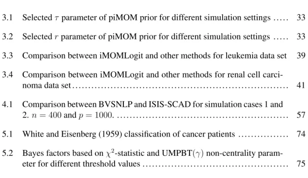
−3 −2 −1 0 1 2 3 0.0 0.2 0.4 0.6 0.8 1.0 β Density

Figure 2.2: Example of overlap between a piMOM prior and approximate normal distri-bution of null MLE coefficients

is determined by a draw from the prior on the model space. For binary outcome datasets, a Bernoulli vector of length n with success probability πˆ is generated, where πˆ is the proportion of successes in the observed data. For survival datasets, survival times have to be estimated. To do this, I use the method discussed in section 4.2.2. Using estimated responses from the null model, the MLE is estimated. This process is repeatedN times to obtain a normal density approximation to the marginal density of the maximum likelihood estimates under the condition that all true regression coefficients (except for the intercept in linear or logistic regression) are 0. Typically,N =O(104).

Next, piMOM priors corresponding to different values ofτ are compared to the null distribution of the MLE. Based on these comparisons, I numerically determine the value of τ so that the overlap of these densities falls below a threshold ofp−1/2_{. This overlap value} is chosen heuristically in a way that suggests the number of false positives will decrease to 0 aspandnbecome large. Other thresholds of the formp−α_{might also be considered,}

(32)

but I have found that α = 1/2provides good performance in a wide range of simulation studies and in real data examples. Further justification for this threshold is provided in section 2.4.1. Figure 2.2 illustrates the overlap between piMOM prior withr = 1.5and τ = 0.6and the approximate normal distribution for null MLE values withσ= 0.43.

Since r controls the tail behavior of the piMOM, I can impose a constraint on the maximum values of estimated coefficients to find an appropriate value for r. For the specific applications discussed in this dissertation, namely logistic regression and the Cox proportional hazard models, it is not sensible to have an absolute value of a coefficient that is more than 10. Therefore I can pick the r value so that |β| falls in the interval

(−10,10) with 95% probability. A numerical strategy for finding this hyperparameter vector is outlined in Algorithm 1 below.

Algorithm 1Choosing Appropriaterandτ for piMOM

1: procedureRTAUSELECT(X, n, p)

2: yn ←Sample from the NULL model 3: for(i in 1:N)do

4: ksize←Sample from prior on model space in (3.4)

5: Xk←Randomly chooseksizecolumns fromX 6: βi ←MLE(yn,Xk)

7: β ←[β βi]

8: f ←Normal density approximation to density ofβ 9: ov←Overlap area betweenf and iMOM(τ, r)

10: tp←Area under iMOM(τ, r)outside the interval(−10,10)

11: [r∗, τ∗]←argmin

r,τ

(|ov−√1_p|+|tp−0.05|)

12: return[r∗, τ∗]

Notice that this procedure for choosing the hyperparameters depends on the prior on the model space. This implies that τ will tend to be larger in larger models, because it is more likely that the sampled columns of X will exhibit high collinearity in large

(33)

models. In addition, I recommend this algorithm for cases wherep≫n, for instance with p > 2n. Otherwise, a very largencan make the distribution of the null MLE very narrow, preventing the desired overlap from being achieved for reasonable values ofτ.

2.4.1 Justification For1/√pOverlap

My rationale for setting the overlap between the sampling distribution of the MLE and the prior density to be p−1/2 _{can be explained as follows. For simplicity, I} mo-tivate my criterion in the context of a scalar-valued parameter θ. Let p(θ) denote the prior density for θ under a nonlocal prior defining the alternative hypothesis,H1, and let f(θ) = ∏n_i=1fi(xi|θ)denote the likelihood function, let i(ˆθ)denote the observed infor-mation evaluated at the MLEθ, i.e.,ˆ

i(ˆθ) =− ∂ 2_log_f₍_θ₎ ∂θ θ=ˆθ . (2.17)

Under the null hypothesis, θ = 0 and therefore under the null model the marginal density of the data is simply m0 = f(0). The marginal likelihood function under the alternative hypothesis can be approximated using Laplace approximation method as

m1(ˆθ)≈

√

2π

i(ˆθ)f(ˆθ)p(ˆθ).

In large samples when the null hypothesis is true,

f(ˆθ)≈f(0)eη(ˆθ)/2, (2.18)

(34)

n, the observed informationi(ˆθ)converges to Fisher’s information,I(0). Definewto be

w=

√

2π

I(0). (2.19)

Now let g(ˆθ) denote the sampling distribution of the maximum likelihood estimate under the null hypothesis. I assume that this sampling density is approximately normally distributed around 0 and let±xdenote the point at which the sampling density of the MLE and the nonlocal prior densities overlap. Under my constraint on the overlap between densities, the expected value ofm1 satisfies

E0[m1(ˆθ)]/w≈ ∫ |_θˆ_|_<x f(0)eη(ˆθ)/2p(ˆθ)g(ˆθ)dθˆ+ ∫ |_θˆ_|_>x f(0)eη(ˆθ)/2p(ˆθ)g(ˆθ)dθˆ ≤max[g(ˆθ)] ∫ |_θˆ_|_<x f(0)eη(ˆθ)/2p(ˆθ) + max[p(ˆθ)] ∫ |_θˆ_|_>x f(0)eη(ˆθ)/2g(ˆθ)dθˆ ≤max[g(ˆθ), p(ˆθ)] [∫ |_θˆ_|_<x f(0)eη(ˆθ)/2p(ˆθ) + ∫ |_θˆ_|_>x f(0)eη(ˆθ)/2g(ˆθ)dθˆ ] ≈max[g(ˆθ), p(ˆθ)]f(0)eη′/2√1 p (2.20) for some random variableη′ that is bounded in probability. The Bayes factor in favor of the larger model is thus

BF10< wmax[g(ˆθ), p(ˆθ)] exp(η′/2)

1

√

p. (2.21)

For largen, the second term on the right hand side of the inequality is determined by the sampling distribution of the MLE and isOp(n1/2), whilewisO(n−1/2). Thus, the average Bayes factor isOp(p−1/2), and combined with the beta-binomial prior on the model space (which imposes a penalty that is O(1/p)on new variables), this suggests that the number

(35)

of false positives under the null model of no effects will decrease to 0 aspincreases. 2.5 Discussion

In this chapter I discussed the hierarchical Bayesian model used in my algorithm to perform high dimensional variable selection. A brief review of the Laplace approximation was also provided in order to compute the marginal probability of the data.

The main idea of my method is the use of nonlocal priors, in particular the piMOM density, for nonzero coefficients. The piMOM density has better behavior around the origin than pMOM density, as well as heavier tails than pMOM, making it suitable for sparse variable selection. An automatic approach for selecting hyperparameters of the piMOM prior was also discussed.

This was a general description of the methodology. The specific details regarding the selection procedure in binary or survival response datasets are provided in the following chapters.

(36)

3. HIGH DIMENSIONAL BAYESIAN VARIABLE SELECTION FOR BINARY RESPONSE DATA∗

3.1 Introduction

Recent developments in bioinformatics and cancer genomics have made it possible to measure thousands of genomic variables that might be associated with the manifestation of cancer. The availability of such data has resulted in a pressing need for the development of statistical methods to use these data to identify variables that are associated with binary outcomes (e.g., cancer or control, survival or death). The topic of this chapter is a statis-tical model for identifying, from a large number p of potential feature vectors, a sparse subset that are useful in predicting a binary outcome vector. Throughout this chapter, I assume that the binary vector of interest is denoted byy, and that the matrix of potential explanatory variables is denoted by X. Along the same lines of (1.1), lettingXk denote

the submatrix ofXcontaining the “true” predictors, I assume that

π =F(Xkβk), (3.1)

whereF denotes a known binary link function (assumed to be the logistic distribution in what follows), andπ is then vector of success probabilities fory. The regression coeffi-cientβkrepresents the non-zero regression effect for each column ofXkin predictingπ.

The primary statistical challenge addressed in this chapter is the selection of the submatrix

Xkto be used for the prediction ofπ.

Different approaches have been proposed to tackle this problem for ultrahigh dimen-∗_{Part of this chapter is reprinted with permission of Oxford University Press, from the article:}

Nikooienejad, A., W. Wang, and V. E. Johnson (2016). Bayesian variable selection for binary outcomes in high-dimensional genomic studies using non-local priors.Bioinformatics 32(9), 1338-1345.

(37)

sional datasets(p≫n)in both Bayesian and frequentist paradigms. Penalized likelihood based methods include the Iterative Sure Independent Screening (ISIS) procedure (Fan and Lv, 2008) which can be applied to different penalty functions such as SCAD (Fan and Li, 2001), LASSO (Tibshirani, 1996) and Dantzig selector (Candes and Tao, 2007). Among Bayesian approaches, Lee et al. (2003) exploit hierarchical probit model with a Gaussian prior for coefficients. West et al. (2000) provided a Bayesian approach to this problem by using informative prior distributions. Liang et al. (2008) studied a mixture ofg priors and Bae and Mallick (2004) considered Gaussian, Jeffery’s and Laplace priors. George and McCulloch (1997) and Rossell et al. (2013) can be listed among methods that utilized discrete mixture priors.

Except for Rossell et al. (2013), each of the Bayesian methods described above impose local prior densities on regression coefficients in the true model. That is, the prior density on the regression coefficients has a positive prior density function at 0 (and in most cases has its mode at 0), which from a Bayesian perspective makes it more difficult to distinguish between models that include regression coefficients that are close to 0 and those that do not. Johnson and Rossell (2012) proposed two new classes of nonlocal prior densities to ameliorate this problem. In the model selection context, nonlocal prior densities are 0 when a regression coefficient in the model is 0. This makes it easier to distinguish between coefficients that do not have an impact on the prediction ofyfrom those that do. Johnson and Rossell (2012) used a Markov Chain Monte Carlo (MCMC) algorithm to sample from the posterior distribution on the model space; the convergence properties of this algorithm were studied in Johnson (2013a).

The primary goal of this chapter is to extend the methodology proposed in Johnson and Rossell (2012) for application to binary outcomes and to compare the performance of this algorithm to leading penalized likelihood methods. In addition, I describe a default procedure for setting the hyperparameters (i.e., tuning parameters) in the nonlocal priors,

(38)

and I examine a numerical strategy for identifying the highest posterior probability model (HPPM).

The remainder of this chapter is structured as follows. In Section 3.2 I describe the MOMLogit variable selection model for binary regression. As part of this description, I propose a default method for setting the hyperparameter values in the nonlocal priors imposed on the regression coefficients, as well as a numerical strategy for estimating the HPPM. The approach for setting the hyperparameter values is new, and is based on com-paring the distribution of the maximum likelihood estimates (MLEs) of randomly selected null models to the nonlocal prior distributions on the regression coefficients. Because the null distribution of the MLEs are centered on 0 and the nonlocal priors decrease to 0 at 0, I show that it is possible to choose model hyperparameters so that the total variation distance between these distributions exceeds a given threshold. Section 3 provides a brief descrip-tion of a computadescrip-tional procedure designed to identify the HPPM. Secdescrip-tion 3.4 presents a simulation study to compare the MOMLogit procedure and ISIS-SCAD algorithm in ultrahigh dimensional settings. My method is then applied to detect genes that are asso-ciated with cancer in that section. Finally Section 3.5 concludes with a discussion of the advantages and disadvantages of the MOMLogit variable selection procedure.

3.2 Methods

Let yn = (y1, . . . , yn)T denote a vector of independent binary observations, Xn an n ×pmatrix of real numbers, β ap×1regression vector, and xi the ith row of Xn. I denote a model byk={k1, . . . , kj}where(1≤k1 <· · ·< kj ≤p)and it is assumed that βk1 ̸= 0, . . . , βkj ̸= 0and all other elements ofβare 0. The design matrix corresponding

to model k is denoted by Xk and is defined to have cardinality k. I assume that the

columns ofXhave been standardized. Theithrow ofXkis denoted byxik. Assuming the

(39)

this chapter is to identify sparse regression models that have high predictive probability. I propose to do this by identifying the highest posterior probability model k for datay, distributed according to yi|βk ∼Bernoulli [ exp(x′_i_kβk) 1 + exp(x′_i_kβk) ] , (3.2)

under prior constraints on the model space and the assumption of nonlocal prior density constraints on the regression parameterβk. My primary focus is on the casep≫n.

Recall from Chapter 2, Bayesian model selection is based on the calculation of pos-terior model probabilities. The pospos-terior probability of model j ∈ J and the marginal probability of the data under modelkwere calculated in (2.4) and (2.5), respectively.

The art in implementing a Bayesian model selection procedure thus focuses on spec-ifying the prior densities πk(βk) for βk under each model, as well as the prior model

probabilitiesp(k)for the models themselves. Except for the intercept, I assume nonlocal priors on the components of the regression vector in each model. For more information on this refer to Section 2.2 in Chapter 2.

3.2.1 Nonlocal Priors

The form of the nonlocal prior densities imposed on the (non-zero) regression coef-ficients βk in this chapter take the form of a product of independent iMOM priors, or

piMOM densities, expressible as

π(βk|τ, r) = τ rk/2 Γ(r/2)k k ∏ i=1 |βi|−(r+1) exp ( − τ β2 i ) . (3.3)

Hereβka vector of coefficients of lengthk, andr, τ > 0. Following what was discussed

in section (2.2) for iMOM priors, the hyperparameterτ represents a scale parameter that determines the dispersion of the prior around0, whileris similar to the shape parameter

(40)

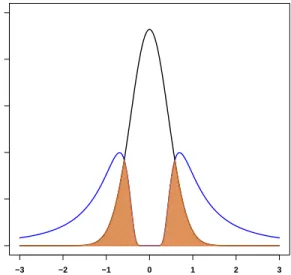
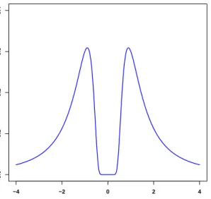
−4 −2 0 2 4 0.0 0.1 0.2 0.3 0.4 β Density

Figure 3.1: piMOM prior forr= 1.5andτ = 1

in Inverse Gamma distribution and determines the tail behavior of the density. An example of piMOM density is illustrated in Figure 3.1 for the particular case ofr = 1.5andτ = 1. 3.2.2 Prior on Model Space

Following from my discussion in Section (2.3.2), I choose a beta-binomial prior as the prior for model size. The formulation specifies that the prior probability for modelkis

p(k) = B(a+k, b+p−k)

B(a, b) , (3.4)

whereB(a, b)denotes the beta function andaandb are prior parameters that describe an underlying beta distribution on the marginal probability that a selected feature is associated with a non-zero regression coefficient in (3.2). This type of prior on the model size is also recommended in Castillo et al. (2015), where it is suggested that an exponential decrease in prior probabilities with model size provides optimal results when the prior density on

(41)

regression parameters has the form of a double exponential.

To incorporate my belief that the optimal predictive models are sparse, I arbitrarily set a = min(k∗,⌊log(p)⌋), andb =p−a. For largen, this implies that I expect, on average, a feature vectors to be included in the model. Here, for the cases that p/n > 4, I pick k∗ = argmax

k

(_p

k

)

< 2n_{, otherwise}_k∗ _{= 8}_{. This choice of} _k∗ _{for the prior} hyperparam-eter reflects the belief that the number of models that can be constructed from available covariates should be smaller than the number of possible binary responses. Similarly, by restrictingato be less thanlog(p), comparatively small prior probabilities are assigned to models that contain more than log(p) covariates. Finally, I impose a deterministic con-straint on model size and defineP(k) = 0ifk > n/2.

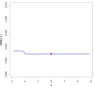
A sensitivity analysis foraandbin (3.4) is provided in Section 3.4.1.1. 3.2.2.1 Choosing Hyperparameters

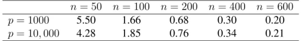
The algorithm for selecting hyperparamters is discussed in details in section 2.4 in chapter (2) and I employ that algorithm here. Notice that for a fixed p, the dispersion of the null distribution of the MLE around 0 decreases as the sample size n increases, although the rate of decrease is also affected by the structure of the design matrixX. This makes the value ofτto decrease in order to maintain a fixed overlap threshold. This effect is illustrated in Table 3.1.

I note that a similar procedure for setting the scale parameter for local priors on the regression coefficients could potentially be implemented. Unfortunately, the application of this procedure to local priors can require extremely large values of the tuning parameters in order to “squash” the prior near 0 and achieve small overlap with the null distribution. As a consequence of this fact, the tuning parameters selected by this procedure will not reflect any reasonable prior belief on the values of the regression parameters in a logistic model with a standardized design matrix.

(42)

Ideally, I would adjust τ for each individual model, but as mentioned earlier it was not computationally feasible to do so for the applications and simulations reported in this chapter.

3.3 Numerical Aspects of Implementation

The model described in section 3.2 leads to a joint density for the data, modelkand its parameters. As a result, the posterior distribution of modelkand its coefficients can be expressed as π(βk,k|yn)∝ τrk/2 Γ(r/2)k k ∏ i=1 |βi|−(r+1)exp ( − τ β2 i ) × B(a+k, b+p−k) B(a, b) n ∏ j=1 { exTjkβk 1 +exTjkβk }yj{ 1 1 +exTjkβk }1−yj . (3.5)

Because of the high dimension of the parameter space and the complexity of the pos-terior density function in (3.5), it is not feasible to maximize this function analytically to obtain the HPPM. To search for the HPPM, I therefore utilized a Markov chain Monte Carlo algorithm. To reduce the dimension of the parameter space, I used a Laplace ap-proximation to marginalize over the regression coefficientβkassociated with each model. The resulting approximation to the marginal posterior density of the datayunder modelk

can be expressed as mk(yn) = ∫ π(yn|βk)πk(βk)dβk≈ (2π)k2|Σ|− 1 2π(y_n|β˜ k)πk(β˜k). (3.6)

Hereβ˜_kis the MAP estimate ofβkand|Σ|is the determinant of the Hessian of the

(43)

on Laplace approximation refer to section 2.3.1.

The elements of the Hessian matrix can be expressed as

Hi,j(βk) =          i=j; −r+1_β2 ik + 6τ β_ik−4+∑ s x2sie x′_skβ_k (1+ex′skβk₎2 i̸=j; ∑ s xsixsjex ′ skβk (1+ex′skβk₎2 . (3.7)

A simple birth-death scheme was used to sample from the posterior distribution. At each iteration of MCMC algorithm, each of thepcovariates was visited in random order. The update at position i was performed by proposing a candidate model by flipping the inclusion state of that variable in the model. The candidate model was accepted using a Metropolis algorithm where the probability of accepting the candidate model,kcand_{, was}

r= mkcand(yn)p(k

cand₎

mkcurr(y_n)p(kcurr)

. (3.8)

The MAP estimate for βk was obtained using the nlminb() function in R. I assumed

that an intercept was present in all models. 3.3.1 Convergence Diagnostics

Convergence diagnostics of MCMC can be used to assess whether an adequate number of iterations have been performed. Because of the high dimension of the parameter space for even moderately largep, I implemented a modified coupling diagnostic (Johnson, 1996, 1998) to assess the probability that my MCMC algorithm had identified the true model. In the standard implementation of this method, one randomly initializes two MCMC chains by independently including each variable in the model according to a fixed probability. The components of the model in each chain are then updated synchronously, using the same uniform random deviate to perform acceptance/rejection of the candidate models. The chains are said to couple when the models from each chain are identical. Note that

(44)

once the chains become coupled, they never uncouple. In theory, the distribution of the number of updates of the chains required to obtain coupling can be used to establish a bound on the Total Variation Distance (TVD) between iterates in the chain and the target distribution.

In my implementation of the coupling diagnostic, I started 100 pairs of model chains. Each pair was updated until either they had coupled or all p components in each of the chains had been updatedN times, whereN = 250. The (local) HPPM identified by each chain was recorded, and then the HPPM’s for the 100 chains were compared. I then iden-tified the global HPPM among the 100 models in the paired chains, and also examined the proportion of chains that had both coupled and identified the “global” HPPM. If the pro-portion was not high enough, it was possible that the paired chains required more updates to reach stationary distribution. This can be checked by increasing the number of updates, N.

This kind of implementation was proposed to overcome a potential convergence issue. Depending on the design matrix, there could be some pairs in which the final model in one chain is different from the final model in the other but the selected models span the same subspace. In this case, the paired chains are never coupled despite converging to same subspace.

3.4 Results

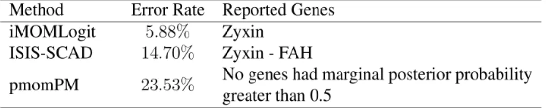
To investigate the performance of the proposed model selection procedure, I applied my procedure to both simulated data sets and real data. I compared the performance of my algorithm to ISIS-SCAD (Fan and Lv, 2008) in both real and simulated data because ISIS-SCAD has proven to be among the most successful model selection procedures used in practice. For the real data analyses, I also compared my method to another Bayesian procedure based on the product moment prior (Rossell et al., 2013).