component based software systems
Viet Hoa Nguyen
To cite this version:
Viet Hoa Nguyen. A model-based method to manage time properties in component based software systems. Software Engineering [cs.SE]. Universit´e Rennes 1, 2013. English. < tel-00923305>
HAL Id: tel-00923305
https://tel.archives-ouvertes.fr/tel-00923305
Submitted on 2 Jan 2014HAL is a multi-disciplinary open access archive for the deposit and dissemination of sci-entific research documents, whether they are pub-lished or not. The documents may come from teaching and research institutions in France or abroad, or from public or private research centers.
L’archive ouverte pluridisciplinaire HAL, est destin´ee au d´epˆot et `a la diffusion de documents scientifiques de niveau recherche, publi´es ou non, ´emanant des ´etablissements d’enseignement et de recherche fran¸cais ou ´etrangers, des laboratoires publics ou priv´es.
THÈSE / UNIVERSITÉ DE RENNES 1
sous le sceau de l’Université Européenne de Bretagne
pour le grade de
DOCTEUR DE L’UNIVERSITÉ DE RENNES 1
Mention : Informatique
Ecole doctorale Matisse
présentée par
Viet-Hoa Nguyen
Préparée à l’unité de recherche
INRIA – Centre Rennes Bretagne Atlantique
Institut National de Recherche en Informatique et Automatique
Une méthode fondée
sur les modèles pour
gérer les propriétés
temporelles des
systèmes à
composants logiciels
Thèse soutenue à Rennes
le 5 Décembre 2013
devant le jury composé de :
Franck BARBIER
Professeur à l’Université de Pau /rapporteur
Philipe COLLET
Professeur à l’Université de Nice / rapporteur
Pascal POIZAT
Professeur à l’Université de Paris Ouest Nanterre /
examinateur
Antoine BEUGNARD
Professeur à l’ENST de Bretagne / examinateur
Jean-Marc JEZEQUEL
Professeur à l’Université de Rennes 1 /
directeur de thèse
Noël PLOUZEAU
Maître de conférences à l’Université de Rennes 1 /
This thesis proposes an approach to integrate the use of time-related stochastic properties in a continuous design process based on models at runtime. Time-related specification of services are an important aspect of component-based architectures, for instance in distributed, volatile networks of computer nodes. The models at runtime approach eases the management of such architectures by maintaining abstract models of architectures synchronized with the physical, distributed execution platform. For self-adapting systems, prediction of delays and throughput of a component assembly is of utmost importance to take adaptation decision and accept evolutions that conform to the specifications. To this aim we define a metamodel extension based on stochastic Petri nets as an internal time model for prediction. We design a library of patterns to ease the specification and prediction of common time properties of models at runtime and make the synchronization of behaviors and structural changes easier. Furthermore, we apply the approach of Aspect-Oriented Modeling to weave the internal time models into timed behavior models of the component and the system. Our prediction engine is fast enough to perform prediction at runtime in a realistic setting and validate models at runtime.
Keywords: Model-Driven Engineering, Performance Prediction, Validation at Runtime
Cette thèse propose une approche pour intégrer l’utilisation des propriétés temporisées stochastiques dans un processus continu de design fondé sur des modèles à l’exécution. La spécification temporelle de services est un aspect important des architectures à base de composants, par exemple dans des réseaux distribués volatiles de nœuds informatiques. L’approche models@runtime facilite la gestion de ces architectures en maintenant des modèles abstraits des archi-tectures synchronisés avec la structure physique de la plate-forme d’exécution distribuée. Pour les systèmes auto-adaptatifs, la prédiction de délais et de débit d’un assemblage de composants est primordial pour prendre la décision d’adaptation et accepter les évolutions qui sont conformes aux spécifications temporelles. Dans ce but, nous définissons une extension du métamodèle fondée sur les réseaux de Petri stochastiques comme un modèle temporisé interne pour la prédiction. Nous concevons une bibliothèque de patrons pour faciliter la spécification et la prédiction des propriétés temporisées classiques de modèles à l’exécution et rendre la synchronisation des comportements et des changements structurels plus facile. D’autre part, nous appliquons l’approche de la modélisation par aspects pour tisser les modèles temporisés internes dans les modèles temporisés de comportement du composant et du système. Notre moteur de prédiction est suffisament rapide pour effectuer la prédiction à l’exécution dans un cadre réaliste et valider des modèles à l’exécution.
Mots clés: Ingénierie Dirigée par les Modèles, Prédiction de Performance, Validation à l’exécution.
First of all, I would like to sincerely thank my advisors, Jean-Marc Jézéquel and Noel Plouzeau, for accepting me as your student and giving me the opportu-nity to pursue my Doctoral studies and working with you and within the Triskell group, one of the best team in the world in the MDE field, and also for guiding and supporting me over the years.
I would also like to thank Prof. Franck BARRIER and Prof. Philippe COL-LET for spending time to review my thesis. Their comments and suggestions helped me to significantly improve my thesis. I would like also thank to my other thesis committee members, Prof. Pascal POIZAT and Prof. Antoine BEUG-NARD for examining my thesis.
Special thanks go to the other members of the Triskell group for providing support and friendship that i needed, with whom i have shared many good mo-ments and interesting discussions. I would also like to thanks all my Vietnamese friends for helping me and staying beside me in difficult times. I am indebted to them for their help.
Finally, i must express my gratitude to my family for their continued support and encouragement, for staying beside my all of the ups and downs of my research.
0.1
Introduction
La conception des logiciels à composants est aujourd’hui une approche bien établie pour la construction de systèmes réutilisables et fiables. Dans ces systèmes, la confiance repose sur les spécifications précises des interfaces des composants et sur l’application des techniques de validation sur des implémentations de composants. Les spécifications comprennent des propriétés de type, des comportements et des propriétés quantitatives [19]. Un système temps réel souple souligne la perfor-mance liée au temps comme une qualité essentielle. Les tâches de spécification de ce genre de système classent le temps de réponse et le débit comme des at-tributs les plus importants du comportement attendu du système. Les architectes en logiciel s’appuient donc sur des techniques d’analyse quantitative pour valider les implémentations par rapport aux spécifications. Cette tâche de validation est principalement une activité faite au moment de la conception, et qui four-nit une prédiction de propriétés quantitatives pour les besoins et les capacités du système avant que ces systèmes soient déployés. Les concepteurs comptent sur ces prédictions pour concevoir une architecture appropriée qui répond aux spécifications, tant qu’un ensemble d’exigences correspondantes reste valable au moment de l’exécution. Les systèmes dits à temps réel souple tels que les sys-tèmes de l’internet des objets (par exemple les réseaux de capteurs intelligents et assistants numériques personnels) sont une classe particulière de systèmes à base de composants, car étant très flexible dans leur conception et configuration. Dans cette thèse, nous nous concentrons sur cette catégorie de systèmes qui sup-porte les changements architecturaux au moment de l’exécution, sans s’arrêter pour se redéployer, mais en effectuant un redéploiement à chaud. Ce genre de système est parfois nommésystème éternel. Le changement architectural est une conséquence de deux causes principales d’évolution : (1) les changements de la définition de service du système ; (2) les changements de l’implémentation du sys-tème. Les changements de la définition de service comprennent les changements de spécification des systèmes du fait de changements des besoins des utilisateurs, par exemple, la suppression ou l’addition de fonctionnalités, des changements
de l’exigence de débit et de temps, les changements de préférences pour la ges-tion d’énergie sur un appareil mobile, etc. Les changements de l’implémentages-tion de service comprennent des changements dans la disponibilité des ressources de l’environnement de soutien du système, par exemple la fluctuation de la bande passante du réseau ou l’addition de nouveaux nœuds de calcul, par exemple les dispositifs mobiles équipés avec les capteurs. Les systèmes de l’internet des ob-jets sont de grands ensembles de nœuds de calcul. Ces systèmes sont oppor-tunistes par conception: pour une application donnée, sa plate-forme d’exécution se compose d’un ensemble de nœuds de calcul en continuelle évolution, avec une puissance de calcul et des capacités de communication très diverses. Par exem-ple, un système social coopératif en temps réel peut connecter les utilisateurs qui partagent des propriétés géographiques (par exemple le cyclisme dans la même ville). Lorsque les utilisateurs se déplacent et changent d’activité leurs assistants personnels numériques se connectent et se déconnectent fréquemment du réseau social, tandis que leurs capacités de communication fluctuent rapidement [93]. Ce genre de système doit être en mesure de se reconfigurer à la volée, souvent en temps réel et de manière autonome, sans nécessiter un redémarrage après la reconfiguration. Ces systèmes ont des caractéristiques architecturales spécifiques, et leurs techniques de conception sont un sujet de recherche actif [27]. Toutefois, la flexibilité ne devrait pas être implémentée au détriment de la perte de fiabilité dans la justesse de ces systèmes adaptatifs. Comme la conceptions de ces systèmes évolue continuellement sans supervision ni intervention humaine, ils doivent aussi mettre en œuvre une auto-validation sans intervention humaine. Par conséquent, un sous-système autonome d’auto-validation doit être présent dans le système auto-adaptatif. Dans cette thèse, nous introduisons un processus de conception et de validation pour la prédiction à la volée des propriétés extra-fonctionnelles liées au temps. Notre approche est triple :
1. Nous intégrons les réseaux de Pétri colorés stochastiques comme une ex-tension du métamodèle pour spécifier les propriétés liées au temps sur les composants.
2. Nous mettons en place une bibliothèque de patrons fréquemment utilisés pour aider les concepteurs à superposer des descriptions de comportement temporisé sur des modèles de services fonctionnels.
3. Nous fournissons une intégration des outils d’évaluation de temps dans les modèles à l’exécution, avec un temps d’évaluation compatible avec des changements rapides dans l’architecture.
0.2
Contributions
Notre approche s’appuie sur le paradigme des models@runtime qui emploient à l’exécution des modèles architecturaux. Nous fournissons des extensions pour gérer les propriétés stochastiques liées au temps (par exemple le délai moyen et
le débit, et le pire cas de temps d’exécution). Plus précisément, nous nous ap-puyons sur des modèles structurels à l’exécution [82] superposés avec des patrons de conception de haut niveau fournissant des descriptions comportementales tem-porisées. Les techniques d’adaptation reposant sur les principes surveiller, anal-yser, planifier et exécuter (MAPE) fonctionnent au niveau de la plate-forme, tan-dis que les modèles à l’exécution supporte des niveaux d’abstraction plus élevés. Le MAPE et les modèles à l’exécution sont complémentaires : en utilisant notre extension d’expression temporelle de propriétés, le MAPE peut utiliser des pro-priétés liées au temps des modèles à l’exécution pour raisonner sur les modèles avant leur déploiement. Réciproquement, les estimations calculées au niveau ab-strait par des algorithmes de prédiction pour les modèles à l’exécution peuvent être comparées aux valeurs réelles obtenues en surveillant la plate-forme après l’exécution du plan de déploiement à chaud.
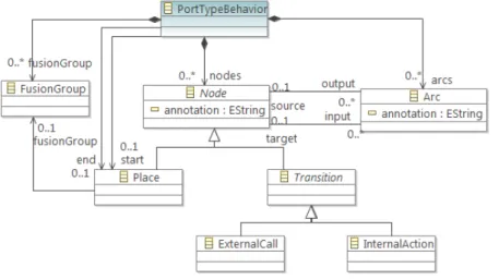
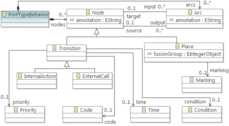
Cependant, la véritable puissance des modèles à l’exécution provient de l’utilisation de la prédiction : quand l’architecture actuelle n’atteint pas l’objectif, les alternatives architecturales doivent être produites et évaluées. Les algorithmes de prédiction peuvent aider à évaluer les propriétés quantitatives de ces architec-tures. Ces algorithmes sont souvent spécialisés et prennent des modèles spécifiques partiels comme les entrées et les sorties, ce qui conduit à nouveau au problème de la correspondance entre le modèle architectural et les modèles de prédiction spécialisés qui sont utilisés par les outils. Notre processus de conception vise à combiner des techniques spécifiques de prédiction quantitative avec des modèles à l’exécution. Pour cela nous nous appuyons sur des extensions du métamod-èle de composants Kevoree [1, 39]. Ces extensions supportent la description de comportements temporels à l’aide de patrons de conception de réseaux de Petri stochastiques colorés. L’extension pour augmenter modèles de composants avec les réseaux de Petri colorés est représentée sur la Figure 3.6. Ces comportements peuvent être associés aux ports de composants (pour des services requis ou four-nis). Ils peuvent être liés aux opérations à partir de la même spécification de composant, ou sur les opérations dans un assemblage d’instances de composants.
0.2.1 Les patrons et le modèle de performance des composants Kevoree
Dans les sections précédentes, nous avons indiqué que la modélisation du com-portement des composants logiciels et des systèmes logiciels en terme de réseaux de Petri colorés s’est avéré être une bonne plate-forme pour capturer des infor-mations critiques dans les systèmes temps réel, réactifs, concurrents et distribués. Toutefois, dans le développement des logiciels modernes, il n’est pas évident que les réseaux de Petri colorés soient familiers aux concepteurs. En conséquence, nous avons défini un ensemble de patrons pour modéliser les réseaux de Petri colorés, dans le but de faciliter le travail des développeurs. Une bibliothèque de patrons peut être établie à partir des expériences acquises en matière de mod-élisation. Les développeurs utilisent souvent des patrons dans la bibliothèque
Figure 1 – Behavior model for Kevoree
pour construire leurs modèles de manière efficace, tout en évitant de réinventer des solutions déjà existantes pour résoudre leurs problèmes. Dans [86], les au-teurs ont proposé un ensemble de 34 modèles de conception empiriques pour la modélisation de systèmes d’information fondés sur les processus et les protocoles de communication pour des systèmes embarqués distribués. Ces modèles servent à résoudre les problèmes qui apparaissent lors de la modélisation au moyen de réseaux de Petri colorés, et ils ont été documentés dans un format qui permet aux concepteurs de comprendre facilement et appliquent ces modèles dans leurs propres problèmes. Les concepteurs doivent déterminer les propriétés recherchées puis construire leurs modèles CPN en utilisant ces patrons.
Pour simplifier le travail des développeurs, nous proposons d’employer des concepts d’interfaces et de paramètres de patrons. Les interfaces d’un patron sont des transitions et des places qui peuvent être connectés avec des transitions et des places externes. Les paramètres du patron sont des informations qui caractérisent une instance du patron. Ces paramètres peuvent être des valeurs de jetons ou le nom de la transition externe (le service requis). En conséquence, l’application d’un patron donné n’est pas faite par copier-coller d’un modèle existant mais par la mise en correspondance des interfaces des patrons avec les éléments existants et la définition des valeurs des paramètres. Ce procédé est analogue aux techniques de conception par aspects. En utilisant le langage de transformation de modèle Kermeta, nous instancions les patrons utilisés à partir du modèle de comportement du composant Kevoree. Dans cette thèse, nous montrons des exemples de patrons pour modéliser les services synchronisés, les chaînes de diffusion de Kevoree.
0.2.2 Composition des modèles
Cette section explique comment composer les modèles de réseaux de Petri col-orés des services de composants, en utilisant l’outil de transformation de modèles
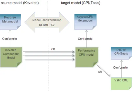
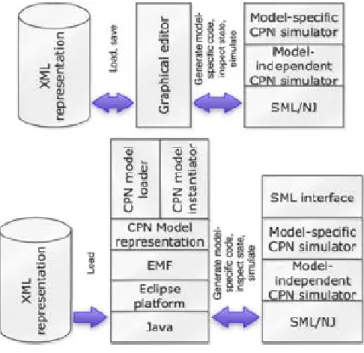
Kermeta. Le résultat de la transformation produit un modèle du système entier qui peut être ensuite être simulé par l’outil CPNtools. Grâce à la similarité de la sémantique de notre métamodèle et de l’outil CPNTools, nous n’avons besoin de considérer que deux problèmes de composition des modèles : comment corre-spondre nos patrons à la sémantique de l’outil CPNTools, et comment gérer les éventuels conflits de la déclaration de variables dans les différent modèles réseaux de Pétri. Une fois les modèles composés, une transformation modèle vers texte est ensuite exécutée pour construire un fichier .cpn qui est conforme au fichier DTD de l’outil CPNTools. La figure 3.27 illustre le processus de transformation du modèle de composant Kevoree vers un modèle CPN du système entier prêt à être simulé.
Comme indiqué dans les sections précédentes, lors d’une adaptation la re-configuration ou la génération de nouveaux modèles des composants Kevoree du système sont réalisées par le système d’analyse d’adaptation. Lors d’une adap-tation un modèle est produit à l’exécution par les algorithme d’adapadap-tation puis évalué par notre système pour déterminer les propriétés quantitatives de ce mod-èle. Le modèle produit doit être conforme métamodèle Kevoree étendu avec notre extension fondée sur les réseaux de Petri. La deuxième étape (# 2) du procédé de transformation est illustrée à la figure 3.27, qui est la transformation du modèle CPN généré dans l’étape (#1) du système entier à un fichier XML qui est com-préhensible par l’outil CPNTools. Ce fichier XML est conforme à la Document Type Definition (DTD) de l’outil CPNTools. Dans cette étape de transformation de modèle vers texte, nous pouvons appliquer d’autres tâches de post-traitement, par exemple l’intégration d’un algorithme de mise en page pour redessiner les éléments de réseaux de Petri.
Le processus de transformation contient deux types différents de transforma-tions :
1. modèle-à-modèle : la transformation d’un modèle conforme à notre mé-tamodèle d’extension vers un modèle global conforme au mémé-tamodèle de réseaux de Pétri colorés compatible avec CPNtools ;
2. modèle-texte : la transformation du précédent modèle vers un fichier XML valide que l’outil CPNtools comprend.
0.3
Conclusion
Cette thèse présente une solution pour rendre prévisible les caractéristiques de performance d’architectures distribués adaptatives . Le travail de cette thèse est fondé sur les principes suivants. Tout d’abord, l’approche proposée repose sur une synthèse automatique des propriétés de performance du système à partir des propriétés des composants correspondants. Deuxièmement, l’approche permet la séparation des préoccupations de propriétés fonctionnelles et extra-fonctionnelles des composants et du système. Troisièmement, elle permet une analyse des
per-Figure 2 – Transformation process from the Kevoree component model to the system-level CPN model
formances efficace en termes de temps d’exécution. Notre cadriciel est complété par un processus de développement et de validation qui guide le développeur de composants et l’analyste de propriétés de qualité de service par un cycle itératif de conception. Ce processus de développement prend en compte des propriétés de performance.
Le cycle itératif comprend les phases suivantes. Une première phase con-struit un certain nombre de modèles de composants en utilisant des bibliothèques disponibles de composants Kevoree. Pour chaque alternative, une deuxième phase compose les modèles de comportement de ces modèles de composants individu-els pour produire un modèle de performance du système global. Une troisième phase réalise l’analyse de ces modèles de performance par rapport aux exigences. Une quatrième et dernière phase permet au moteur de raisonnement de choisir la meilleure alternative à partir des résultats d’analyse et de réaliser la reconfigura-tion à partir de ce choix.
L’approche proposée dans cette thèse offre les avantages suivants.
• Conformément aux principes de l’ingénierie des modèles, au moment de la conception un architecte peut travailler sur les modèles de comportement correspondantes des composants, définir le modèle de performance atten-due du système et procéder à l’analyse de la performance, avec un niveau d’abstraction égal à celui des propriétés fonctionnelles du système en cours de conception.
• L’analyse des propriétés de performance d’un modèle s’opère dans un délai compatible avec une adaptation continue du système ayant lieu plusieurs fois par minute.
• La bibliothèque de patron de conception contenant des descriptions types de modèles de performance et de comportement accélère la phase de conception et évite le recours à un expert en réseaux de Petri stochastiques.
.
• L’emploi de modèles paramétrés à aspect pour la description des patrons de conception est compatible avec les pratiques de la conception par aspects. • L’emploi de réseaux de Pétri colorés offre une grande puissance d’expression
Abstract i
Résumé iii
Acknowledgements v
Résumé en français vii
0.1 Introduction . . . vii
0.2 Contributions . . . viii
0.2.1 Les patrons et le modèle de performance des composants Kevoree . . . ix
0.2.2 Composition des modèles . . . x
0.3 Conclusion . . . xi
1 Introduction 1 1.1 Introduction . . . 1
1.2 Research questions . . . 3
1.3 Thesis outline . . . 3
2 State of the art 7 2.1 Dynamic component-based software engineering . . . 7
2.1.1 Component-based approach . . . 7
2.1.2 Reusable components . . . 8
2.1.3 Component model . . . 9
2.1.4 Extra-functional properties modeling of component-based technologies 9 2.1.5 Model-driven engineering . . . 11
2.1.6 Models at runtime . . . 13
2.1.7 Kevoree framework . . . 14
2.1.7.1 Dynamic adaptation modeling . . . 14
2.1.7.2 Models at runtime . . . 15
2.1.7.3 Kevoree metamodel . . . 15
2.2 Methods for performance evaluation of software systems . . . 18
2.2.1 Analysis and validation of software models . . . 18
2.2.2.1 Model checking . . . 19
2.2.2.2 Theorem proving . . . 19
2.2.3 Quantitative analysis . . . 19
2.2.3.1 Performance aspects . . . 20
2.2.3.2 Performance models . . . 20
2.3 Performance prediction approaches for component-based systems . . . 23
2.3.1 Performance prediction methods . . . 23
2.3.1.1 Prediction approaches based on UML . . . 24
2.3.1.2 Prediction approaches based on specific metamodels or formal definitions . . . 26
2.3.2 Prediction approaches based on measurement . . . 29
2.3.3 Colored Petri nets and CPNtools . . . 30
2.3.3.1 Colored Petri nets . . . 30
2.3.3.2 Stochastic Petri nets for component-based system design . . 30
2.3.3.3 Time analysis . . . 32
2.3.3.4 Access/CPN . . . 32
2.4 State-of-the-Art summary . . . 33
3 Performance prediction model for Kevoree 35 3.1 Development and validation process model . . . 36
3.2 Behavior model for Kevoree components . . . 39
3.2.1 Behavioral CPN meta-model . . . 39
3.2.2 Color type declaration of interface places . . . 41
3.2.3 Performance indicators injection . . . 43
3.3 Parameterized templates and aspect-oriented modeling . . . 46
3.3.1 Aspect-oriented modeling . . . 46
3.3.2 Measurement model . . . 49
3.4 Parameterized CPN templates for Kevoree . . . 53
3.4.1 Introduction of parameterized templates . . . 55
3.4.2 Synchronous service call template . . . 56
3.4.3 Broadcast channel pattern . . . 57
3.5 Model composition and mapping from CPN-Kevoree model to Access/CPN model . . . 62
4 Experiment and validation 73 4.1 Component model of the application . . . 73
4.2 Behavior models of individual components and of the whole system . . . 74
4.3 Measuring performance aspects . . . 81
4.3.1 Notification delay time monitor . . . 81
4.3.2 Conclusion . . . 83
5 Conclusion 85 5.1 Discussion on Research Questions . . . 87
1 Behavior model for Kevoree . . . x
2 Transformation process from the Kevoree component model to the system-level CPN model . . . xii
1.1 Overview of the thesis structure . . . 4
2.1 Non-functional properties of software systems . . . 12
2.2 A model transformation . . . 12
2.3 Art dynamic adaptation model . . . 15
2.4 Model at runtime . . . 16
2.5 Kevoree topology model . . . 17
2.6 Kevoree type definition . . . 17
2.7 Overview of prediction methods . . . 24
2.8 The most abstract model . . . 31
2.9 Network . . . 32
2.10 Access/CPN tools . . . 33
3.1 Behavior model specification. . . 36
3.2 Validation at runtime process . . . 37
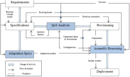
3.3 Self-adaptive component-based development process model with QoS analysis 38 3.4 QoS analysis workflow . . . 39
3.5 Integration of behavior modeling into Kevoree . . . 40
3.6 Behavior model for Kevoree . . . 40
3.7 Monitor of CPN nets for capturing QoS measures of the simulation . . . 41
3.8 Types used to modeling the CPN behavior models . . . 42
3.9 Declarations of color sets and variables defined in the model . . . 42
3.10 An example of color type declaring convention . . . 43
3.11 Assembly of A and B components . . . 46
3.12 Different roles in QoS-driven development process . . . 47
3.13 Component performance modeling process based on aspect-oriented modeling 47 3.14 Model composition and validation process on active nodes at runtime . . . . 48
3.15 The components of the QoS evaluation model . . . 49
3.16 An example of a measurement model defining the response time aspect . . . . 50
3.18 The declarations used for the monitor of response time . . . 51
3.19 Application of CPN template in Kevoree . . . 55
3.20 Synchronous service call template . . . 58
3.21 The Response Time measurement associated with the Synchronous Service Call template . . . 58
3.22 The application of theSynchronous Service Call template . . . 58
3.23 The model after applyingSynchronous Service Call template . . . 59
3.24 The final result after applyingSynchronous Service Call template and associ-ated Response Time measurement . . . 59
3.25 Broadcast Channel Pattern. . . 63
3.26 Definition of a monitor to measure the bandwidth of the channel instance . . 64
3.27 Transformation process from the Kevoree component model to the system-level CPN model . . . 65
3.28 CPN model composition derived from component model . . . 65
3.29 Module for generating the XML code that the CPNtools unerstands . . . 70
4.1 Kevoree component model of the temperature’s firefighters application. . . 74
4.2 The class diagram of the temperature’s firefighters application. . . 74
4.3 The CPN model at top-level generated by Kermeta and derived from the Kevoree component model of the system. . . 75
4.4 The timed behavior model of the alarm service of the alarm component, de-veloped by third parties. . . 76
4.5 The CPN model of the alarm service derived after the transformation step. . 77
4.6 The CPN model after the transformation of the Channel 1 instance imple-mented in node 1. . . 78
4.7 The CPN model of the notify service port. . . 78
4.8 The timed behavior model of thecapture service port. . . 80 5.1 The state-space formal model checking to verify the generated configuration . 89
Introduction
1.1
Introduction
Component-based software design is now a well established approach for building reusable and trust-able systems. In these systems, trust relies on precise specifications of component interfaces and on application of validation techniques on component implementations. Speci-fications include typing properties, behaviors and quantitative properties [19]. Soft real-time systems emphasize time related performance as a vital quality. Specifications for this kind of system rank response time and throughput as first class attributes of the expected system behavior. Designers therefore rely on quantitative analysis techniques to validate implemen-tations against specifications. This validation task is mainly a design time activity, which provides prediction of quantitative properties for the system’s needs and capabilities before these systems are deployed. Designers rely on these predictions to engineer an appropriate architecture that will meet the specifications, as long as a set of corresponding requirements remains valid at run time. Soft real time systems such as Internet of Things systems (e.g. networks of smart sensors and personal digital assistants) are a particular class of component based systems, being highly flexible in their design and configuration. In this thesis we fo-cus on this category of systems that must support major architectural changes at run-time, without stopping but instead by hot-deploying. Such a kind of systems are sometimes named eternal systems. Architectural changes are a consequence of two main evolution causes: (1) changes of system’s service definition; (2) changes of system’s implementation. Changes of service definition include changes of systems specification stemming from changes of user’s needs, for instance addition or removal of functionality, changes in timing and throughput requirements, changes of preferences for power management on a mobile device, etc. Changes of service implementation include changes in resource availability from the supporting envi-ronment of the system, for instance fluctuations of network bandwidth, or addition of new computation nodes e.g. sensor equipped mobiles.
Internet of Things systems are large sets of computation nodes. These systems are oppor-tunistic by design: for a given application, its execution platform is made of a continuously evolving set of computation nodes, with very diverse computing power and communication capabilities. For example, a real time cooperative social system can connect users that share geographical properties (e.g. cycling in the same city). As users move and switch activities, their personal digital assistants frequently connect to and disconnect from the social network, while their communication capabilities fluctuate rapidly [93]. Such systems must be able to reconfigure on the fly, and even self reconfigurable in real time, without requiring a restart after reconfiguration. These systems have specific architectural features, and their design techniques are an active research topic [27]. However, flexibility should not be implemented at the expense of loss of trust in the correctness of these adaptive systems. As these system’s designs evolve continuously without human supervision and intervention, they must also im-plement self validation without human intervention. Therefore an autonomous self-validation subsystem must be present in the self-adapting system.
To address the challenging issues discussed above, we propose to apply a formal language to the design and analysis of real-time adaptive systems. We also propose to use Model-Driven Engineering (MDE)[55] for an automatic evaluation process. MDE enables the formal specification of performance-relevant models of components; these models serve as an input into an automatic composition engine that assembles sub-models into a performance-relevant system-level model. Analyzing this system-level model will provide the reasoning engine with predictions on system quality attributes, including performance.
The problem of performance prediction of component-based assembly is a challenging task. Predictable Assembly (PA) [101] allows assembling at early design time a system out of individual independent-developed arbitrary components with predictable functional and extra-functional properties. Once the assembly is realized, and the attributes of individual components are available, the quality of the attributes of the assembly could be reasoned. In general, the process of performance prediction of component-based systems at design time requires the following tasks:
1. Modeling the functional behavior tailored with performance properties of individual components
2. Identifying the assembly structure and mapping scheme on hardware platforms 3. Analyzing and reasoning about the performance properties of the assembly.
A number of Component-based Software Engineering (CBSE) performance prediction methods have emerged during the last decades, such as PALLADIO [12], KLAPER [44]. A detailed analysis and comparison of these approaches is presented in section 2.3. However, most of them do not tackle the problem of performance evaluation at run-time, which is needed to support the continuous reconfiguration of modern adaptive distributed systems. Based on that analysis, we identify the following aspects that are important for supporting runtime performance evaluation:
• Modeling semantics for specifications of various performance properties of individual components. A third-party software component could be deployed in different
environ-ments. The need to consider its potential execution environments and incorporate them into the system performance modeling makes the problem more difficult. Additionally, modeling of complex systems needs a powerful formalism , for instance, the ability of concurrency, synchronization, and mutual exclusion of shared resource modeling, etc. • Well-defined semantics and rules for assembling the performance-related models of
in-dividual components in an automatic way. The performance specification of software components and assemblies is a basic problem that must be solved to enable system assembly out of individual components. The description of performance aspects of the system-level mode should be derived from that of individual components, so that the system-level model could be available for analysis and the performance aspects of the whole system will be measured.
• Reasoning framework allowing to extract and analyze the performance analysis results. The performance results should be reasoned in a perfect time to adapt to the continuous changes of highly adaptive systems.
• Time-effect performance analysis for performance evaluation of alternative configura-tions. Using models-at-runtime more than one configurations must be evaluated, lead-ing to more computation time for evaluation.
1.2
Research questions
Based on the above discussion, we consider a number of research questions that need to be addressed in this thesis:
Research Question 1 How should the functional and performance properties of individual independent-developed components be specified in order to enable automated compo-sition of these properties and to capture all environment aspects which may influence the performance of the components?
Research Question 2 How to evaluate performance properties of combined system archi-tectures at run time in an automatic way?
Research Question 3 How can the reasoning engine compare architectural alternatives and select an optimized one with respect to multiple quality attributes?
Research Question 4 Can this approach proposed in this thesis be applied to others sys-tems, such as embedded real-time systems ones?
Research Question 5 How can other extra-functional properties like security, availability, etc be expressed and evaluated?
1.3
Thesis outline
Figure 1.1 – Overview of the thesis structure
• We integrate stochastic colored Petri nets as a metamodel extension for specifying time-related component properties (Section 3.2).
• We set up a library of frequently used patterns to help designers to superimpose timed behavior descriptions on functional models (Section 3.3). These patterns also map timing evaluation results back into higher level system models.
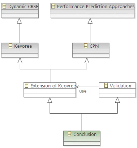
• We provide an integration of timing evaluation tools in the models at runtime paradigm (Chapter 3), with an evaluation time compatible with rapid changes in the architecture. Figure 1.1 gives an overview of the thesis structure. Figure 1.1 gives the contents of my thesis and the relations between different parts in my thesis. The light grey elements present the background and State-of-the-Art parts of the thesis. The white elements represent the description of methodology, framework, and ours contributions.
The remainder of the thesis is organized as follows:
• Chapter 2 presents the background in dynamic component-based software development and performance prediction approaches. Chapter 2 consists of three subsections. The
first subsection 2.1 (the Dynamic CBSE element in the top left-hand side of Figure 1.1) introduces fundamentals of component-based software engineering and provides back-ground information on Model-driven software development and Models@Runtime. The second subsection 2.2 introduces different methods of performance analysis. Finally, the third subsection 2.3 (the Performance Prediction Approaches element in the top right-hand side) gives a survey on approaches for performance predictions of component-based systems.
• Chapter 3 first formulates the performance-oriented development process in the Kevoree framework. We then discuss in detail the extension of the Kevoree framework for performance prediction.
• Chapter 4 describes the validation part of the thesis. In this chapter, the approach is validated through a case study that is implemented based on our proposed framework. • Chapter 5 concludes the thesis and presents perspectives. In this chapter, we discuss the advantages and drawbacks of the approach and then we list some open issues and we propose future work to response the research question #3.
State of the art
This chapter presents the background and concepts that are needed to understand the rest of the thesis, and then discusses some related approaches. This chapter consists of three subsections.
The first section 2.1 introduces basics in the areas of component-based software en-gineering and background information on Model-driven software development and Mod-els@Runtime. This section also defines the different types of extra-functional properties of component-based technologies. At the end of this section, an overview of the Kevoree framework is presented.
In the second section 2.2), we introduce different methods of performance analysis. This section also clarifies the difference between quantitative and qualitative analysis. At the end of the section, we introduce the concepts pertaining to coloured Petri nets, the CPNtools and Access/CPN software. We define a metamodel extension based on stochastic Petri nets as an internal time model for prediction.
The third section 2.3 gives a survey on approaches for performance predictions of component-based systems. Through this section, the drawbacks and advantages of each approach are also analyzed.
2.1
Dynamic component-based software engineering
2.1.1 Component-based approach
There are several proven advantages of the component-based approach. A major advantage of the component-based approach is that it allows for the rapid construction of qualified applications with reusable components, the facility of maintainability and the dynamic of applications [112] [43] [30] [51]. A deeper explanation of concepts such as component, com-ponent assembly, and comcom-ponent framework will be presented in the next sections. Benefits of the component-based approach can be summarized as follows:
Extendability Legacy software systems are difficult to extend. Due to the development of legacy software systems as monolithic systems, new functionalities must be inserted directly into the source code, and the whole program must be then rebuilt, whereas component-based systems can be updated and extended easily by adding new compo-nents or updating existing ones.
Reduced time-to-market The component developers can focus only on the construction of the functionality of the component, without taking into account system resource allocation, because a component framework provides other runtime services commonly needed by components.
Predictability All design rules and patterns of the whole system are defined by the compo-nent model, which is then enforced for each compocompo-nent. For that reason, it is unlikely to make a mistake in the design of a whole system.
2.1.2 Reusable components
The definitions of components vary and there has not been a unique general definition of what a component is so far. First, we refer to one of the precise definitions of components [102]: A software component is a unit of composition with contractually specified interfaces and explicit context dependencies only. A software component can be deployed independently and is subject to composition by third parties. Another definition of the components in [8] states that the component is an opaque implementation of functionality, subject to third-party composition and conforming to a component model. There exist different types of the components depending on the design purposes. We distinguish three types of component: Black-box, White-box and Grey-box.
Black-box is generally a part of a program which provides a functionality, in which users know only inputs and outputs. The users call the functions with inputs and expect outputs. The inner implementation of the functionality remains hidden. In contrast, White-box allows the users to have access to the inner architecture or source code, it makes called white-box. White-box makes generally the replacement of an old program by new one [102] more prob-lematic. From the white-box point of view, users of components may study the source code of the program, so that users may adjust programs. For example, users change a sequence of calls, modify somehow input and output values to obtain a better performance of the program. Components designed as black-boxes are more convenient for future replacement. Since the components’ primary goal is to be replaceable, it even more highlights the need for black-box components. One point worth noting here is that there exist several component-based approaches where components designed as grey-box that aim at improving the predictability of extra-functional properties [15]. For instance, the Palladio component designs [12] include Service Effect Specification (SEFF) to model performance-relevant information together with behavior model of the component. Users have access to the SEFF models of the components but not to the source code of the component, so that the component assembler may select convenient components for their design goals, for example, to obtain a component assembly that satisfies some performance requirements of the final system. The selection of components is based on interfaces of components and information from SEFF models.
2.1.3 Component model
The component-based approach consists in designing and developing systems by assembling reusable components. It is composed of an assembly of prefabricated, preconceived, pretested components and interconnected by contracts, and required and provided interfaces. To con-struct a component-based system, the developers rely on reusable components instead of creating new ones from scratch. The component model gives a uniformity to components and their composition. Its use is to define how a component should look like, how com-ponents communicate between each other, and which resources they use. The component model ensures that the components are compatible in terms of deployment, communication. It determines the rules that components must follow to be able to cooperate and its min-imal misunderstood assumptions. Another goal of usage of the component model is the predictability. The component model may define typical software requirements, for example, to avoid deadlock, manages race-conditions, synchronization. The component model may also support extra-functional properties such as performance-relevant properties, memory consumption. Paper [8] claims that the component model should provide:
A component type expressed by interfaces that the component implements. When the component implements more interfaces its type is made of the types of all implemented interfaces. In other words the component is polymorphic with respect to all imple-mented interfaces. A component type is basically a factory for building component instances. The identification and design of the component type are performed by the business experts and the architects of the system following classical software engineering techniques.
An interaction mechanism used by the component model to specify how components are located, which communication protocols are used; it may also define which level of quality of services is achieved.
A resource binding description describing how each deployed component is bound to some resources. A resource is provided by a framework, in which the component is deployed, or by other components. The component model describes which components are available and how the components bind to them. Consequently, the component model drives the life cycle of components and manages resource assignment.
2.1.4 Extra-functional properties modeling of component-based technolo-gies
The main objective of this section is to present the notion of extra-functional properties of software systems. Even when a particular functional requirement of a component is satisfied, the functionality of the component in the target environment may not be guaranteed unless all extra-functional requirements are fulfilled. From the users’ point of view, there are two disjunctive parts to be considered:
1. functions, for which the component has been developed for; 2. a set of extra-functional properties of the component.
The correctly working function developed in the component may not be enough in the target environment. It is useful to allow users to take into account extra-functional requirements of the component to fulfill users’ needs. For that reason, it is important to express relevant extra-functional properties of the components. While the specification of extra-functional properties is well understood in current industrial models and frameworks, most of them lack the support of extra-functional properties. A functionality of published components does not depend on whether they are able to guarantee their function with regard to specific extra-functional requirements. Let us point out that the termextra-functional propertieslacks a standardized definition.
The work in [19] does not define precisely extra-functional properties, but the authors define a general model software contract. The extra-functional properties are derived from extra-functional aspects, by specifying constraints over the values of extra-functional aspects. They divide contracts into four levels of increasingly negotiable properties:
Syntactic level This first level of contract is required simply to make the system work. In this level, the designers specify functions that their components can perform.
Behavior level . This second level improves the level of confidence in sequential context by defining the requirements and outcome of operations. For instance, the Eiffel language [77] allows for the definition of pre-conditions and post-conditions to capture conditions that must hold to ensure a result of the computation. The other example is theassert
command in the Java language. This construct is used to check the validity of input parameters of methods. Behavioral contracts can also be expressed by means of the contract expressed using UML and OCL (Object Contraint Language) [107] formalism.
Synchronization level The third level improves confidence in distributed or concurrency contexts. This level of contract concerns all aspects connected with multi-threaded computation.
Quality of service level The fourth level quantifies quality of service. Quality of service includes attributes such as maximum response time, delay, average response time, mem-ory usage. They are mainly relevant in resolving whether the whole component system will meet extra-functional requirements when executed on a given platform.
This classification does not cover all kinds of quality requirements. Extra-functional requirement includes all expected quality characteristics from a user’s point of view. extra-functional requirement could be divided into different sets such as quality of service, behavior, synchronization, etc. Generally, we can describe the association of these sets as below:
Behavior + synchronization + QoS requirements ⊂extra-functional requirement.
It is useful to precisely and formally describe all relevant extra-functional properties of components since it allows checking whether a component matches extra-functional require-ments. An active research activity has been devoted to formal definitions of extra-functional properties such as HQML (Hierarchical QoS Markup Language) [47], TADL (Architecture Description Language for Trustworthy Component-Based systems) [79], QML [41], CQML [2]. When component compatibility checks are improved by extra-functional properties, it leads to more precise decisions on whether one component is suitable as a replacement for the other
one. Chapter 4 will present approaches and their underlying analysis methods that support extra-functional properties expression and prediction.
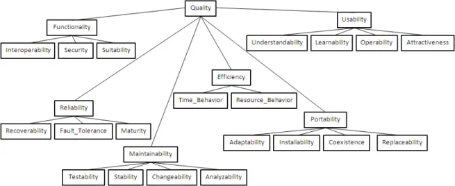
In short, extra-functional requirements are the requirements that specify criteria that can be used to analyze the operation of a system, rather than a specific behavior. Typical extra-functional requirements are reliability, scalability, and cost. Extra-extra-functional requirements are also known as constraints, quality attributes, and time constrained responses and availability of required service. Temporal properties are considered as hypothesis on the behavior of the system. Figure 2.1 is an example of a quality model presented in [38] to define the quality of software systems. The quality model is explained with the help of six main factors and several subfactors:
Functionality is defined as a set of attributes that deal with the existence of a set of functions and their specified properties. The functions are those that satisfy stated or implied needs.
Reliability is defined as a set of attributes that deal with the capability of software to maintain its level of performance under stated conditions for stated period of time.
Efficiency is a set of attributes that deal with the relationship between the level of perfor-mance of software and the amount of resources used, under stated conditions.
Usability is a set of attributes that deal with the effort needed for use, and on the individual assessment of such use, by a stated or implied set of users.
Maintainability is a set of attributes that deal with the effort needed to make specified modifications.
Portability is a set of attributes that deal with the ability of software to be transferred to from one environment to another.
There exist several other quality models such as [22] or [73].
2.1.5 Model-driven engineering
MDE is a software development methodology that focuses on abstracting some aspects of reality for a given purpose by creating and exploiting domain models for this purpose. Figure 2.2 shows the Meta Object Facility (MOF) pyramid-shaped structure [103]. The metamodel describes the concepts and relationships of a given domain. Each model in Figure 2.2 conforms to the well-defined metamodel. The first level model in the pyramid-shaped structure is the meta-metamodel that conforms to MOF, which is self-described. The metamodel is the most important part of a Domain-Specific Modeling Language (DSML). It defines concepts in the domain. For the purpose of designing metamodels, there exists EMF (Eclipse Modeling Framework) [5], which is ade-facto standard modeling framework.
From a model specification described in XMI, EMF provides tools and runtime support to produce a set of Java classes for the model, a set of adapter classes that enable viewing and command-based editing of the model, and a basic editor. We can also use EMFText [10] to create the textual syntax of a DSML or the GMF (Graphical Modeling Framework)
Figure 2.1 – Non-functional properties of software systems
Figure 2.2 – A model transformation
[11] to construct a graphical syntax. Tools and frameworks such as Kermeta [55] provide static and dynamic semantic of metamodel. Kermeta provides OCL-like syntax to specify static semantics, such as the constraints the models must obey. Kermeta allows designing invariants and pre/post-conditions. The conventional modeling framework like EMF does not allow the definition of behavior in operations integrated into a metamodel. Kermeta allows aspect-oriented modeling, which helps design pre/post-conditions, variants and behaviors of a metamodel.
MDE provides a variety of software processes to allow the creation of modeling domains and the transformation of its models. The Model-driven Architecture (MDA™) marketed by the Object Management Group (OMG) presents a model-driven approach to system develop-ment. The MDA defines two principle model levels, Platform Independent Model (PIM) and Platform Specific Model (PSM). The former specifies an application independent of the plat-form technologies, but only the specification of business layer of the application. The latter specifies an application in a specific modeling domain. The platform independent models are incrementally transformed and refined into lower-level platform specific models. The PSMs are then transformed into implementation artifacts such as implementation code. This
ap-proach of automatic construction of systems from high-level models is based on the principle of model transformation.
The Model transformation is another important aspect of MDE. Amodel transformation
takes input models conforming to an input metamodel M M1 and produces output models
conforming the output metamodel M M0 as illustrated in Figure 2.2. A transformation is
basically an ensemble of rules to implement a mapping between elements in source model and elements in target model. The model transformation may transform models within the same modeling domain (endogenous transformations) or between different modeling domains (exogenous transformations). There exists a number of model transformation languages such as Kermeta [85], rule-based ATL [56] [57], graph grammar based AToM [105]. Different types of model transformation can be created using model transformation languages. Such types of transformation are Model-to-Model transformation and Model-to-Text transforma-tion. Model-to-Model transformation is a transformation mechanism that transforms a source model into a target model. The source and target models conform to their respective meta-model. Model-to-text transformation transforms a model into text, which is normally the source code. The next section presents the models@runtime approach, which is based on the model-driven engineering.
2.1.6 Models at runtime
Adaptive systems are often expected to adapt to the changes in their execution environment. Hence, self-adaptive systems require to adapt their behavior and their structure at runtime with little or no human intervention. Models@runtime [81] [21] has emerged as a promising approach to develop adaptive systems. An advantage of using models@runtime is to develop adaptation mechanisms that leverage software models to manage complexity in runtime envi-ronments. The basic idea of models@runtime is to apply the model-driven engineering (MDE) approaches to the runtime environment. At a first glance, models@runtime may be considered as a reflection concept. The reflection deals with causally connected, self-representations of an underlying system. The models should mirror the system, its current state and behavior. If the system changes, the models should change and vice versa. However, in the reflection research domain, models are often related to the computation model and hence tend to be based on the implementation space and rather low level. In models@runtime, models are on a much higher level of abstraction, and they are causally connected models related to the problem space. Another key point of models@runtime approach is that models should be intrinsically tied to the models produced from the MDE process. The work in [21] defines the models@runtime concept: a models@runtime is a causally connected self-representation of the associated system that emphasizes the structure, behavior or goals of the system from a problem space perspective. Runtime models provide abstractions of runtime phe-nomena. There are several benefits of runtime models such as dynamic state monitoring, control of systems during execution, dynamic observation of the runtime behavior to under-stand a behavioral phenomenon. Now that we have introduced the model-driven engineering and the models@runtime approaches, the next section presents the Kevoree framework that is dedicated to a technique based on models at runtime that enables dynamic adaptation for distributed component-based systems. The metamodel extension proposed in Chapter
4 based on stochastic Petri nets is integrated into Kevoree metamodel as an internal time model for prediction.
2.1.7 Kevoree framework
The Kevoree framework [1] is dedicated to a technique based on models@runtime that enables dynamic adaptation for distributed component-based systems. This framework supports ho-mogeneous continuous design of dynamic distributed component-based software architecture and an intelligent reflection layer that allows evaluating new configurations without stop-ping the current running system. The Kevoree project was inspired by the EUT-ICT DiVA project (Dynamic Variability in complex, Adaptive systems; www.ict-diva.eu), which is a first attempt to enhance reflection with models@runtime. The rest of this section discusses the kernel of the framework-dynamic adaptation mechanism, and the Kevoree component model that provides concepts to describe the underlying infrastructure of distributed component-based systems.
2.1.7.1 Dynamic adaptation modeling
The approach uses software models at runtime as well as at design time to cope with two main difficulties related to adaptation management and evolution management. The first difficulty is coping with the variability that can lead to explosion of several adaptive artifacts. The set of possible configurations of an adaptive system is specified by identifying variation points, which represents points in the software where variability may occur. The number of configurations explodes in a combinatorial way w.r.t the number of variants, and the number of possible configuration transitions is quadratic w.r.t the number of configurations. The second difficulty is the evolution of the adaptive system. Evolving an adaptive system means dynamically changing the adaptation state machine (adding and removing states and transitions). The modifications to the adaptation state machine leads to the redeployment and restart of the new configuration. The DiVA project uses an adaptation metamodel to assist in modeling the DSPL (dynamic software product line) at design time [83] [36]. Models conforming to adaptation metamodel are the main data manipulated by the runtime infrastructure responsible for dynamically adapting component-based applications at runtime. These models provide a high-level basis for reasoning about relevant aspects of the system and its environment and offer enough details to fully automate the dynamic adaptation process. It is possible to make the design specifications evolve at any time, before initial deployment or while the system is already running. Figure 2.3 presents the concepts of the approach, which includes the architecture of the system in the right hand side and the adaptation layer managing the dynamic variability in the left hand side.
For the architecture model, designers can use existing modeling languages, such as the Unified Modeling Language (UML) or Service Component Definition Language from the Ser-vice Component Architecture (SCA), or any architecture description language, to describe the architecture. The approach uses Aspect-oriented modeling (AOM) technique to represent the variability in the architecture model; leaf features of the DSPL model are modeled as aspects, which can be woven or not in the application. The adaptation model captures the
Figure 2.3 – Art dynamic adaptation model
dynamic variability information, i.e. which functionality should be used depending on the context. The adaptation model includes four different aspects: variants, adaptation rules, dependencies, and context. The variant aspects and constraints (requires, excludes) among variants are modeled using feature models. The context aspects specify the system’s environ-ment. A set of variables specifies those aspects of the environment relevant to adaptation. At runtime, the variable values are provided by context sensors, and these may trigger a system reconfiguration. The adaptation rules part of the reasoning model describes selection of the variability features according to context. The approach investigates two different formalisms to capture the adaptation rules, which are event-condition-action (ECA) [33] [59] rules and goal-based optimization rules [48].
2.1.7.2 Models at runtime
Kevoree usesmodels@runtimeto enable intelligent reflection for distributed component-based systems. As discussed in previous sections, models@runtime relies on model-driven ap-proaches to cope with the complexity of dynamic adaptation. The conventional reflection approaches often offer reflection APIs to support the introspection of the system and dy-namic adaptation (by applying CRUD operations on elements of the system). In a nutshell, models@runtime is a reflection model that is uncoupled with runtime system and modeled at a higher-level abstraction. This model allows validation of new configurations, checks when changes appear, without modifying the running system. The new configurations are compared with the current configuration, which is a mirror that reflects the running system. The adaptation model represents a set of commands to transform the current configura-tion into the new configuraconfigura-tion. The adaptaconfigura-tion engine implements these commands at the platform level. If a concrete action execution fails than the adaptation engine rollbacks the configuration to its previous state. Figure 2.4 shows the adaptation mechanism of Kevoree.
2.1.7.3 Kevoree metamodel
The Kevoree metamodel [32] supports many features to allow models@runtime on top of a distributed component platforms:
Figure 2.4 – Model at runtime
approaches that synchronize operations on reflection model and runtime. Contrarily, uncoupled mode allows working on reflection models without modifying the running systems.
2. Type and instance separation.
3. Closed isolation of components: closed isolation of components means that for each couple of components binding together, they can not execute the code of each other. This property is to ensure the capacity of halting a component without influences on other processes.
4. Dynamic provisioning: capacity to dynamically integrate executable code to a running system.
5. Distributed topology model.
6. Channel type: to describe complex semantics of component bindings. This subsection presents a subset of the elements of the Kevoree metamodel.
Node, NodeType: Figure 2.5 shows a part of Kevoree metamodel related to distributed topology model. The Node element describes a logical node in distributed systems. ANode
can be a container of component instances, channels and other nodes. This allows a hierar-chical modeling in Kevoree, whereas the parent node is responsible for starting and stopping its child nodes.
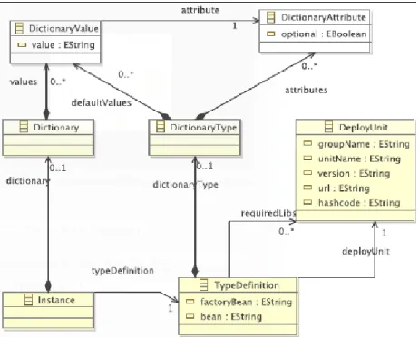
Type definitions, Instances: Figure 2.6 shows elements related to type definitions. A
TypeDefinition element contains third party dependencies (DeployUnit). DictionaryType
defines the parameters of the component type. Each instance refers to its type definition. Component instances are bounded together through bindings and channels. Component and
Figure 2.5 – Kevoree topology model
2.2
Methods for performance evaluation of software systems
2.2.1 Analysis and validation of software models
This section discusses validation or analysis of the system model. There are two aspects to consider when analyzing a system model: the qualitative aspects and quantitative aspects. The analysis of the whole system aims at providing qualitative and quantitative information of the system behavior [3] [46] [74] [50] [62] [61]:
• qualitative analysis aims at ensuring that the properties of the system correspond to the expected properties, for instance the absence of bottleneck, the reachability of a specific state;
• quantitative analysis and performance evaluation aims at quantifying the performance of the system w.r.t the objectives of the system. The performance aspects may be the response time of the users requests, the average delay of the message transmission in a communication network, the bandwidth of transactions in data based systems, etc. In recent years, verification techniques and performance evaluation are used increasingly in industry to analyze a variety of systems such as real-time systems, embedded systems, adaptive systems. These techniques have proved their efficiency. For the purpose of verifi-cation of extra-functional properties, including performance-related of a system, the analysis methodology can be initially subdivided into two approaches: measurement-based and model-based approaches. The former comprises three distinct fields: measurements, benchmarks, prototypes. This technique requires the availability of either the system to be suited or its approximation, so that it can be observed. During the design process, before the imple-mentation phase, measurements on real systems are obviously not applicable, and prototype implementations are very difficult because of the necessity of specifying many details that are far from being decided. The state-of-the-art review in this thesis concentrates on the latter one, which can be partitioned into two types: simulation models and analytical models. This technique can be applied during the early system design phase. In the case of analytical models, the description is given in mathematical terms, whereas in the case of simulation models the description is given by means of a computer program. The simulation will almost always deliver results that are less accurate than the ones that can be obtained by using ana-lytical models, and model complexity of very large systems may cause considerable negative impact on simulation time [98]. The advantage of simulation over analytic modeling is that very detailed system behaviors can be captured. The analytic modeling requires much more constraints in modeling. In other words, simulation allows the development of more detailed models, whereas analytically models are normally more abstract. Additionally, models can be either deterministic or probabilistic. It may be simpler and more realistic to model the systems by means of probabilistic assumptions due to the fact that the details are often not known, and even when they are, their inclusion may lead to very complex models. Fur-thermore, the probabilistic approach may be advantageous because it may provide sufficient accuracy, while yielding more general results.
2.2.2 Qualitative analysis
Quantitative analysis and verification aims at analyzing the qualified properties of the systems [13] [114] We distinguish three classes of verification techniques: model checking, proving, and test.
Properties to verify: there are several types of property that can be verified [30]. The properties listed below are some examples:
• Reachability: to verify that in some conditions, whether a state of the system can be reached or not, for example, whether an initial state may be attained, a state of availability of resources, etc.
• Liveness: the properties that cannot be checked on finite executions (they need to be checked on infinite executions).
• Safety: the properties that can be checked on finite executions. For example, it can-not happen that both processes are in their critical sections simultaneously (mutual exclusion).
• Deadlock free: it ensures that the system never reach a blocked state where it cannot quit.
2.2.2.1 Model checking
The verification or model checking [71] relies on the construction of a finite model of the system, which is then used to check whether a specified property is correct in this model or not. This method is considerably automatic and rapid. In general, the way to perform this verification is to verify that a property expressed in terms of temporal logic is correct in the system. The model checker always proceeds by exploring the state space, whatever the formalism used to model the system. In most cases, the model checkers give the positive response if the property is guaranteed for all the behaviors of the system, and a negative response completed with a counterexample in case of violation of the property.
2.2.2.2 Theorem proving
Theorem proving consists in expressing the system and their properties in terms of a mathe-matical logic and then researching a proof of these properties. This approach is precise, but it requires user intervention. The theorem proving can be applied to all phases of development of the system [49] [91].
2.2.3 Quantitative analysis
Quantitative analysis aims at computing quantitative performance-relevant parameters. The methods of performance evaluation are based on mathematical fundamentals, more precisely theory of probability and Markovian stochastic processes. The performance evaluation con-sists of the following steps:
1. describe the static and dynamic aspects of the system under study by using formal models;
2. analyze the system by generating the state space. The state space is computed as a stochastic process, for example, a Markov chain;
3. resolve the obtained chain to compute the probability of each state in the chain; 4. compute the performance aspects based on probabilities obtained.
2.2.3.1 Performance aspects
The Markovian methods in [29, 25, 60] allow different kinds of analysis: transitory and stationary analysis. The calculated performance aspects give information of efficiency and productivity of the system. On the contrary, transitory and stationary analysis answer to questions such as: in a long period, what is the usage of the server (the percentage of time the server is busy). For these two kinds of analysis, there are frequently a set of the calculated performance aspects: the throughput (the number of request per time unit), the average of response time (the average time to execute a user request of the system), the average of waiting time (the average of time the request has to wait in a queue), resource usage (the percentage of time in average the resource is busy), the frequency of the executions of a task, etc.
2.2.3.2 Performance models Markovian process:
Markovian processes [29, 25] represent a class of stochastic processes. A stochastic process is a family of random variables{x(t), t∈T}defined on a given probability