GeoDa: An Introduction to Spatial Data
Analysis
Luc Anselin
1, Ibnu Syabri
2, Youngihn Kho
11Spatial Analysis Laboratory, Department of Geography, University of Illinois, Urbana, IL,2Laboratory for
Spatial Computing and Analysis, Department of Regional and City Planning, Institut Teknologi, Bandung, Indonesia
This article presents an overview ofGeoDaTM, a free software program intended to serve as a user-friendly and graphical introduction to spatial analysis for non-geographic information systems (GIS) specialists. It includes functionality ranging from simple mapping to exploratory data analysis, the visualization of global and local spatial autocorrelation, and spatial regression. A key feature ofGeoDais an interactive environment that combines maps with statistical graphics, using the technology of dynamically linked windows. A brief review of the software design is given, as well as some illustrative examples that highlight distinctive features of the program in applications dealing with public health, economic development, real estate analysis, and criminology.
Introduction
The development of specialized software for spatial data analysis has seen rapid growth as the lack of such tools was lamented in the late 1980s by Haining (1989) and cited as a major impediment to the adoption and use of spatial statistics by geographic information systems (GIS) researchers. Initially, attention tended to focus on conceptual issues, such as how to integrate spatial statistical methods and a GIS environment (loosely versus tightly coupled, embedded versus modular, etc.), and which techniques would be most fruitfully included in such a framework. Familiar reviews of these issues are represented in, among others, Anselin and Getis (1992); Goodchild et al. (1992); Fischer and Nijkamp (1993); Fotheringham and Rogerson (1993, 1994); Fischer, Scholten, and Unwin (1996); and Fischer and Getis (1997). Today, the situation is quite different, and a fairly substantial collection of spatial data analysis software is readily available, ranging from niche programs, customized scripts and extensions for commercial statistical and GIS packages, to a
Correspondence: Luc Anselin, Department of Geography, University of Illinois, Urbana-Champaign, Urbana, IL 61801
e-mail: [email protected]
burgeoning open-source effort using software environments such as R, Java, and Python. This is exemplified by the growing contents of the software tools clearing house maintained by the U.S.-based Center for Spatially Integrated Social Science (CSISS).1
CSISS was established in 1999 as a research infrastructure project funded by the U.S. National Science Foundation in order to promote a spatial analytical perspec-tive in the social sciences (Goodchild et al. 2000). It was readily recognized that a major instrument in disseminating and facilitating spatial data analysis would be an easy-to-use, visual, and interactive software package aimed at the non-GIS user and requiring as little as possible in terms of other software (such as GIS or statistical packages).GeoDais the outcome of this effort. It is envisaged as an ‘‘introduction to spatial data analysis’’ where the latter is taken to consist of visualization, explora-tion, and explanation ofinterestingpatterns in geographic data.
The main objective of the software is to provide the user with a natural path through an empirical spatial data analysis exercise, starting with simple mapping and geovisualization, moving on to exploration, spatial autocorrelation analysis, and ending up with spatial regression. In many respects,GeoDais a reinvention of the originalSpaceStatpackage (Anselin 1992), which by now has become quite dated, with only a rudimentary user interface, an antiquated architecture, and performance constraints for medium and large data sets. The software was rede-signed and rewritten from scratch, around the central concept of dynamically linked graphics. This means that different ‘‘views’’ of the data are represented as graphs, maps, or tables with selected observations in one highlighted in all. In that respect, GeoDais similar to a number of other modern spatial data analysis software tools, although it is quite distinct in its combination of user friendliness with an extensive range of incorporated methods. A few illustrative comparisons will help clarify its position in the current spatial analysis software landscape.
In terms of the range of spatial statistical techniques included,GeoDais most alike to the collection of functions developed in the open-source R environment. For example, descriptive spatial autocorrelation measures, rate smoothing, and spatial regression are included in thespdeppackage, as described by Bivand and Gebhardt (2000), Bivand (2002a,b), and Bivand and Portnov (2004). In contrast to R,GeoDais completely driven by a point and click interface and does not require any programming. It also has more extensive mapping capability (still somewhat experimental in R) and full linking and brushing in dynamic graphics, which is currently not possible in R due to limitations in its architecture. On the other hand,
GeoDa is not (yet) customizable or extensible by the user, which is one of the strengths of the R environment. In that sense, the two are seen as highly complementary, ideally with more sophisticated users ‘‘graduating’’ to R after being introduced to the techniques inGeoDa.2
The use of dynamic linking and brushing as a central organizing technique for data visualization has a strong tradition in exploratory data analysis (EDA), going back to the notion of linked scatter plot brushing (Stuetzle 1987) and various
methods for dynamic graphics outlined in Cleveland and McGill (1988). In geographical analysis, the concept of ‘‘geographic brushing’’ was introduced by Monmonier (1989) and made operational in theSpider/Regardtoolboxes of Haslett, Unwin, and associates (Haslett, Wills, and Unwin 1990; Unwin 1994). Several modern toolkits for exploratory spatial data analysis (ESDA) also incorporate dynamic linking, and, to a lesser extent, brushing. Some of these rely on interaction with a GIS for the map component, such as the linked frameworks combining XGobi or XploRe with ArcView (Cook et al. 1996, 1997; Symanzik et al. 2000); the SAGE toolbox, which uses ArcInfo (Wise, Haining, and Ma 2001); and the DynESDA extension for ArcView (Anselin 2000),GeoDa’s immediate predecessor. Linking in these implementations is constrained by the architecture of the GIS, which limits the linking process to a single map (inGeoDa, there is no limit on the number of linked maps). In this respect, GeoDa is similar to other freestanding modern implementations of ESDA, such as the cartographic data visualizer, orcdv
(Dykes 1997), GeoVISTA Studio (Takatsuka and Gahegan 2002), and STARS (Rey and Janikas 2006). These all include functionality for dynamic linking, and to a lesser extent, brushing. They are built in open-source programming environments, such as Tkl/Tk (cdv), Java (GeoVISTA Studio), or Python (STARS) and thus easily extensible and customizable. In contrast,GeoDais (still) a closed box, but of these packages it provides the most extensive and flexible form of dynamic linking and brushing for both graphs and maps.
Common spatial autocorrelation statistics, such as Moran’sIand even the Local Moran, are increasingly part of spatial analysis software, ranging from CrimeStat
(Levine 2006), to thespdepand DClusterpackages available on the open-source comprehensive R archive network (CRAN),3as well as commercial packages, such as the spatial statistics toolbox of the forthcoming release of ArcGIS 9.0 (ESRI 2004). However, at this point in time, none of these include the range and ease of construction of spatial weights or the capacity to carry out sensitivity analysis and visualization of these statistics contained in GeoDa. Apart from the R spdep
package, Geoda is the only one to contain functionality for spatial regression modeling among the software mentioned here.
A prototype version of the software (known asDynESDA) has been in limited circulation since early 2001 (Anselin, Syabri, and Smirnov 2002a; Anselin et al. 2002b), but the first official release of a beta version of GeoDa occurred on February 5, 2002. The program is available for free and can be downloaded from the CSISS software tools Web site (http://geoda.uiuc.edu).The most recent version, 0.9.5-i, was released in January 2003. The software has been well received for both teaching and research use and has a rapidly growing body of users. For example, by the fall of 2005, there were more than 8000 registered users, increasing at a rate of about 200 new users per month.
In the remainder of the article, we first outline the design and briefly review the overall functionality ofGeoDa. This is followed by a series of illustrative examples, highlighting features of the mapping and geovisualization capabilities, exploration
in multivariate EDA, spatial autocorrelation analysis, and spatial regression. The article closes with some comments regarding future directions in the development of the software.
Design and functionality
The design ofGeoDaconsists of an interactive environment that combines maps with statistical graphs, using the technology of dynamically linked windows. It is geared to the analysis ofdiscretegeospatial data, that is, objects characterized by their location in space either as points (point coordinates) or polygons (polygon boundary coordinates). The current version adheres to ESRI’s shape file as the standard for storing spatial information. It contains functionality to read and write such files, as well as to convert ASCII text input files for point coordinates or boundary file coordinates to the shape file format. It uses ESRI’s MapObjects LT2 technology for spatial data access, mapping, and querying. The analytical function-ality is implemented in a modular fashion, as a collection of C11 classes with associated methods.
In broad terms, the functionality can be classified into six categories:
spatial data manipulation and utilities: data input, output, and conversion,
data transformation: variable transformations and creation of new variables,
mapping: choropleth maps, cartogram and map animation,
EDA: statistical graphics,
spatial autocorrelation: global and local spatial autocorrelation statistics, with inference and visualization,
spatial regression: diagnostics and maximum likelihood estimation of linear spatial regression models.
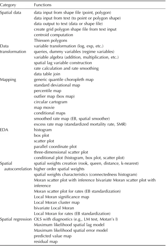
The full set of functions is listed in Table 1 and is documented in detail in the
GeoDauser’s guides (Anselin 2003, 2004)4
The software implementation consists of two important components: the user interface and graphics windows on the one hand and the computational engine on the other hand. In the current version, all graphic windows are based on Microsoft Foundation Classes (MFC) and thus are limited to MS Windows platforms.5 In contrast, the computational engine (including statistical operations, randomization, and spatial regression) is pure C11code and largely cross platform.
The bulk of the graphical interface implements five basic classes of windows: histogram, box plot, scatter plot (including the Moran scatter plot), map, and grid (for the table selection and calculations). The choropleth maps, including the significance and cluster maps for the local indicators of spatial autocorrelation (LISA), are derived from MapObjects classes. Three additional types of maps were developed from scratch and do not use MapObjects: the map movie (map animation), the cartogram, and the conditional maps. The three-dimensional scatter plot is implemented with the OpenGL library.
Table 1 GeoDaFunctionality Overview Category Functions
Spatial data data input from shape file (point, polygon) data input from text (to point or polygon shape) data output to text (data or shape file)
create grid polygon shape file from text input centroid computation
Thiessen polygons Data
transformation
variable transformation (log, exp, etc.) queries, dummy variables (regime variables) variable algebra (addition, multiplication, etc.) spatial lag variable construction
rate calculation and rate smoothing data table join
Mapping generic quantile choropleth map standard deviational map percentile map
outlier map (box map) circular cartogram map movie conditional maps
smoothed rate map (EB, spatial smoother)
excess rate map (standardized mortality rate, SMR)
EDA histogram
box plot scatter plot
parallel coordinate plot three-dimensional scatter plot
conditional plot (histogram, box plot, scatter plot) Spatial
autocorrelation
spatial weights creation (rook, queen, distance, k-nearest) higher order spatial weights
spatial weights characteristics (connectedness histogram)
Moran scatter plot with inference bivariate Moran scatter plot with inference
Moran scatter plot for rates (EB standardization) Local Moran significance map
Local Moran cluster map bivariate Local Moran
Local Moran for rates (EB standardization) Spatial regression OLS with diagnostics (e.g., LM test, Motan’s I)
Maximum likelihood spatial lag model Maximum likelihood spatial error model predicted value map
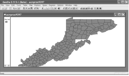
The functionality ofGeoDais invoked either through menu items or directly by clicking toolbar buttons, as illustrated in Fig. 1. A number of specific applications are highlighted in the following sections, focusing on some distinctive features of the software.
Mapping and geovisualization
The bulk of the mapping and geovisualization functionality consists of a collection of specialized choropleth maps, focused on highlighting outliers in the data, so-calledbox maps(Anselin 1999). In addition, considerable capability is included to deal with the intrinsic variance instability of rates, in the form of empirical Bayes (EB) or spatial smoothers.6 As mentioned in ‘‘Design and functionality,’’ the mapping operations use the classes contained in ESRI’s MapObjects, extended with the capability for linking and brushing. GeoDa also includes a circular cartogram,7 map animation in the form of a map movie, and conditional maps. The latter are nine micro-choropleth maps constructed by conditioning on three intervals for two conditioning variables, using the principles outlined in Becker, Cleveland, and Shyu (1996) and Carr et al. (2002).8 In contrast to the traditional choropleth maps, the cartogram, map movie, and conditional maps do not use MapObjects classes, and were developed from scratch.
We illustrate the rate smoothing procedure, outlier maps and linking opera-tions. The objective in this analysis is to identify locations that have elevated mortality rates and to assess the sensitivity of the designation as outlier to the effect of rate smoothing. Using data on prostate cancer mortality in 156 counties contained in the Appalachian Cancer Network (ACN) for the period 1993–97,
we construct a box map by specifying the number of deaths as the numerator and the population as the denominator.9 The resulting map for the crude rates (i.e., without any adjustments for differing age distributions or other relevant factors) is shown as the upper-left panel in Fig. 2. Three counties are identified asoutliersand shown in dark red.10These match the outliersselectedin the box plot in the lower-left panel of the figure. Thelinkingof all maps and graphs results in those counties also being cross-hatched on the maps.
The upper-right panel in the figure represents a smoothed rate map, where the rates were transformed by means of an Empirical Bayes procedure to remove the effect of the varying population at risk. As a result, the original outliers are no longer, but a different county is identified as having elevated risk. Also, a lower outlier is found as well, shown as dark blue in the box map.11Note that the upper outlier is barely distinguishable, due to the small area of the county in question. This is a common problem when working with admininistrative units. In order to remove the potentially misleading effect of area on the perception of interesting patterns, a circular cartogram is shown in the lower-right panel of Fig. 2, where the area of the circles is proportional to the value of the EB smoothed rate. The upper outlier is shown as a red circle, the lower outlier as a blue circle. The yellow circles are the counties that were outliers in the crude rate map, highlighted here as a result of linking with the other maps and graphs.12
Figure 2. Linked box maps, box plot, and cartogram, raw and smoothed prostate cancer mortality rates.
Multivariate EDA
Multivariate exploratory data analysis is implemented in GeoDa through linking and brushing between a collection of statistical graphs. These include the usual histogram, box plot, and scatter plot, but also a parallel coordinate plot (PCP) and three-dimensional scatter plot, as well as conditional plots (conditional histogram, box plot, and scatter plot).
We illustrate some of this functionality with an exploration of the relationships between economic growth and initial development, typical of the recent ‘‘spatial’’ regional convergence literature (for an overview see Rey 2004). We use economic data over the period 1980–99 for 145 European regions, most of them at the NUTS II level of spatial aggregation, except for a few at the NUTS I level (for Luxembourg and the United Kingdom).13
Fig. 3 illustrates the various linked plots and map. The left-hand panel contains a simple percentile map (GDP per capita in 1989), and a three-dimensional scatter plot (for the percent agricultural and manufacturing employment in 1989 as well as the GDP growth rate over the period 1980–99). In the top right-hand panel is a PCP for the growth rates in the two periods of interest (1980–89 and 1989–99) and the GDP per capita in the base year, the typical components of a convergence regression. In the bottom of the right-hand panel is a simple scatter plot of the growth rate in the full period (1980–99) on the base year GDP.
Both plots on the right-hand side illustrate the typical empirical phenomenon that higher GDP at the start of the period is associated with a lower growth rate. However, as demonstrated in the PCP (some of the lines suggest a positive relation between GDP and growth rate), the pattern is not uniform and there is a suggestion of heterogeneity. A further exploration of this heterogeneity can be carried out by brushing any one of these graphs. For example, in Fig. 3, a selection box in the three-dimensional scatter plot is moved around (brushing) which highlights the selected observations in the map (cross-hatched) and in the PCP, clearly showing opposite patterns in subsets of the selection. Furthermore, in the scatter plot, the slope of the regression line can be recalculated for a subset of the data without the selected locations, to assess the sensitivity of the slope to those observations. In the example shown here, the effect on convergence over the whole period is minimal (0.147 versus 0.144), but other selections show a more pronounced effect. Further exploration of these patterns does suggest a degree of spatial heterogeneity in the convergence results (for a detailed investigation, see Le Gallo and Dall’erba 2003).
Spatial autocorrelation analysis
Spatial autocorrelation analysis includes tests and visualization of both global (test for clustering) and local (test for clusters) Moran’s I statistic. The global test is visualized by means of a Moran scatter plot (Anselin 1996), in which the slope of the regression line corresponds to Moran’sI. Significance is based on a permutation test. The traditional univariate Moran scatter plot has been extended to depict bivariate spatial autocorrelation as well, that is, the correlation between one variable at a location, and a different variable at the neighboring locations (Anselin, Syabri, and Smirnov 2002a). In addition, there also is an option to standardize rates for the potentially biasing effect of variance instability (see Assunc¸a˜o and Reis 1999).
Local analysis is based on the Local Moran statistic (Anselin 1995), visualized in the form of significance and cluster maps. It also includes several options for sensitivity analysis, such as changing the number of permutations (to as many as 9999), rerunning the permutations several times, and changing the significance cutoff value. This provides an ad hoc approach to assess the sensitivity of the results to problems due to multiple comparisons (i.e., how stable is the indication of clusters or outliers when the significance barrier is lowered).
The maps depict the locations with significant Local Moran statistics (LISA significance maps) and classify those locations by type of association (LISA cluster maps). Both types of maps are available for brushing and linking. In addition to these two maps, the standard output of a LISA analysis includes a Moran scatter plot and a box plot depicting the distribution of the local statistic. Similar to the Moran scatter plot, the LISA concept has also been extended to a bivariate setup and includes an option to standardize for variance instability of rates.
The functionality for spatial autocorrelation analysis is rounded out by a range of operations to construct spatial weights, using either boundary files (contiguity based) or point locations (distance based). A connectivity histogram helps in identifying potential problems with the neighbor structure, such as ‘‘islands’’ (locations without neighbors).
We illustrate spatial autocorrelation analysis with a study of the spatial distribution of 692 house sales prices for 1997 in Seattle, WA. This is part of a broader investigation into the effect of subsidized housing on the real estate market.14For the purposes of this example, we only focus on the univariate spatial distribution, and the location of any significant clusters or spatial outliers in the data.
The original house sales data are for point locations, which, for the purposes of this analysis are converted to Thiessen polygons. This allows a definition of ‘‘neighbor’’ based on common boundaries between the Thiessen polygons. On the left-hand panel of Fig. 4, two LISA cluster maps are shown, depicting the locations of significant Local Moran’s I statistics, classified by type of spatial association. The dark red and dark blue locations are indications of spatialclusters
(respectively, high surrounded by high, and low surrounded by low).15In contrast, the light red and light blue are indications of spatial outliers (respectively, high surrounded by low, and low surrounded by high). The bottom map uses the default
significance ofP50.05, whereas the top map is based onP50.01 (after carrying out 9999 permutations). The matchingsignificance map is in the top right-hand panel of Fig. 4. Significance is indicated by darker shades of green, with the darkest corresponding to P50.0001. Note how the tighter significance criterion elemi-nates some (but not that many) locations from the map. In the bottom right-hand panel of the figure, the corresponding Moran scatter plot is shown, with the most extreme ‘‘high–high’’ locations selected. These are shown as cross-hatched poly-gons in the maps, and almost all obtain highly significant (at P50.0001) local Moran’sIstatistics.
The overall pattern depicts a cluster of high priced houses on the East side, with a cluster of low priced houses following an axis through the center. Put in context, this is not surprising as the East side represents houses with a lake view, while the center cluster follows a highway axis and generally corresponds with a lower income neighborhood. Interestingly, the pattern is not uniform, and several spatial outliers can be distinguished. Further investigation of these patterns would require a full hedonic regression analysis.
Spatial regression
As of version 0.9.5-i,GeoDa also includes a limited degree of spatial regression functionality. The basic diagnostics for spatial autocorrelation, heteroskedasticity and nonnormality, are implemented for the standard ordinary least-squares regres-sion. Estimation of the spatial lag and spatial error models is supported by means of the maximum likelihood (ML) method (see Anselin and Bera 1998, for a review of the technical issues). In addition to the estimation itself, predicted values and residuals are calculated and made available for mapping.
The ML estimation in GeoDa distinguishes itself by the use of extremely efficient algorithms that allow the estimation of models for very large data sets. The standard eigenvalue simplification is used (Ord 1975) for data sets up to 1000 observations. Beyond that, the sparse algorithm of Smirnov and Anselin (2001) is used, which exploits the characteristic polynomial associated with the spatial weights matrix. This algorithm allows estimation of very large data sets in reason-able time. In addition,GeoDaimplements the recent algorithm of Smirnov (2003) to compute the asymptotic variance matrix for all the model coefficients (i.e., including both the spatial and nonspatial coefficients). This involves the inversion of a matrix of the dimensions of the data sets. To date,GeoDais the only software that provides such estimates for large data sets.
All estimation methods employ sparse spatial weights, but they are currently constrained to weights that are intrinsically symmetric (e.g., excludingk-nearest neighbor weights). The regression routines have been successfully applied to real data sets of more than 300,000 observations (with estimation and inference completed in a few minutes). By comparison, a spatial regression for the 30001
We illustrate the spatial regression capabilities with a partial replication and extension of the homicide model used in Baller et al. (2001) and Messner and Anselin (2004). These studies assessed the extent to which a classic regression specification, well-known in the criminology literature, is robust to the explicit consideration of spatial effects. The model relates county homicide rates to a number of socioeconomic explanatory variables. In the original study, a full ML analysis of all the U.S. continental counties was precluded by the constraints on the eigenvalue-basedSpaceStatroutines. Instead, attention focused on two subsets of the data containing 1412 counties in the U.S. South and 1673 counties in the non-South.
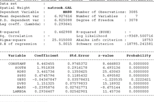
In Fig. 5, we show the result of the ML estimation of a spatial error model of county homicide rates for the complete set of 3085 continental U.S. counties in 1980. The explanatory variables are the same as before: a Southern dummy
variable, a resource deprivation index, a population structure indicator, unemploy-ment rate, divorce rate, and median age.16
The results confirm a strong positive and significant spatial autoregressive coefficientð^l¼0:29Þ. Relative to the OLS results (e.g., Messner and Anselin 2004, Table 7.1., p. 137), the coefficient for unemployment has become insignificant, illustrating the misleading effect spatial error autocorrelation may have on infer-ence using OLS estimates. The model diagnostics also suggest a continued presinfer-ence of problems with heteroskedasticity. However,GeoDacurrently does not include functionality to deal with this.
Future directions
GeoDais a work in progress and still under active development. This development proceeds along three fronts. First and foremost is an effort to make the code cross-platform and open source. This requires considerable change in the graphical interface, moving from the MFC that are standard in the various MS Windows flavors, to a cross-platform alternative. The current efforts use wxWidgets,17which operates on the same code base with a native GUI flavor in Windows, MacOSX and Linux/Unix. Making the code open source is currently precluded by the reliance on proprietary code in ESRI’s MapObjects. Moreover, this involves more than simply making the source code available, but entails considerable reorganization and streamlining of code (refactoring), to make it possible for the community to effectively participate in the development process.
A second strand of development concerns the spatial regression functionality. While currently still fairly rudimentary, the inclusion of estimators other than ML and the extension to models for spatial panel data are in progress. Finally, the functionality for ESDA itself is being extended to data models other than the discrete locations in the ‘‘lattice’’ case. Specifically, exploratory variography is being added, as well as the exploration of patterns in flow data.
Given its initial rate of adoption, there is a strong indication that GeoDa is indeed providing the ‘‘introduction to spatial data analysis’’ that makes it possible for growing numbers of social scientists to be exposed to an explicit spatial perspective. Future development of the software should enhance this capability and it is hoped that the move to an open source environment will involve an international community of like-minded developers in this venture.
Acknowledgements
This research was supported in part by U.S. National Science Foundation Grant BCS-9978058, to the Center for Spatially Integrated Social Science (CSISS) and by grant RO1 CA 95949-01 from the National Cancer Institute. In addition, this research was made possible in part through a Cooperative Agreement between the Center for Disease Control and Prevention (CDC) and the Association of Teachers of Preventive Medicine (ATPM), award number TS-1125. The contents
of the article are the responsibility of the authors and do not necessarily reflect the official views of NSF, NCI, the CDC, or ATPM. Special thanks go to Oleg Smirnov for his assistance with the implementation of the spatial regression routines and to Julie Le Gallo and Julia Koschinsky for preparing the data set for the European convergence study and for the Seattle house prices, respectively. GeoDaTM is a trademark of Luc Anselin.
Notes
1 See http://www.csiss.org/clearinghouse/
2 Note that the CSISS spatial tools project is an active participant in the development of spatial data analysis methods in R, see, for example, http://sal.uiuc.edu/csiss/Rgeo/ 3 http://cran.r-project.org/
4 A Quicktime movie with a demonstration of the main features can be found at http:// sal.uiuc.edu/movies/GeoDaDemo.mov
5 Ongoing development concerns the porting of all MFC-based classes to a cross-platform architecture, using wxWidgets. See also ‘‘Future directions’’ at the end of this article. 6 The EB procedure is due to Clayton and Kaldor (1987); see also Marshall (1991) and
Bailey and Gatrell (1995, pp. 303–08). For an alternative recent software
implementation, see Anselin, Kim, and Syabri (2004). Spatial smoothing is discussed at length in Kafadar (1996).
7 The cartogram is constructed using the nonlinear cellular automata algorithm due to Dorling (1996).
8 The conditional maps are part of a larger set of conditional plots, which includes histograms, box plots, and scatter plots.
9 Data obtained from the National Cancer Institute SEER (Surveillance, Epidemiology, and End Results) web site, http://seer.cancer.gov/seerstat/
10 The respective counties are Cumberland, KY, Pocahontas, WV, and Forest, PA. 11 The new upper outlier is Ohio county, WV; the lower outlier is Centre county, PA. 12 Note that the outliers identified may be misleading as the rate analyzed is not adjusted for
differences in age distribution. In other words, the outliers shown may simply be counties with a larger proportion of older males. A much more detailed analysis is necessary before any policy conclusions may be drawn.
13 The data are from the most recent version of the NewCronos Regio database by Eurostat. NUTS stands for ‘‘Nomenclature of Territorial Units for Statistics’’ and contains the definition of administrative regions in the EU member states. NUTS II level regions are roughly comparable with counties in the U.S. context and are available for all but two countries. Luxembourg constitutes only a single region. For the United Kingdom, data is not available at the NUTS II level, as these regions do not correspond to local
governmental units.
14 The data are from the King County (Washington State) Department of Assessments. 15 More precisely, the locations highlighted show the ‘‘core’’ of a cluster. The cluster itself
can be thought of as consisting of the core as well as the neighbors. Clearly some of these clusters are overlapping.
16 See the original articles for technical details and data sources. In Baller et al. (2001), a different set of spatial weights was used than in this example, but the conclusions of the
specification tests are the same. Specifically, using the county contiguity, the robust Lagrange Multiplier tests are 1.24 for the Lag alternative, and 24.88 for the Error alternative, strongly suggesting the latter as the proper alternative.
17 http://www.wxwidgets.org
References
Anselin, L. (1992).SpaceStat, a Software Program for Analysis of Spatial Data. Santa Barbara, CA: National Center for Geographic Information and Analysis (NCGIA), University of California.
Anselin, L. (1995). ‘‘Local Indicators of Spatial Association—LISA.’’Geographical Analysis
27, 93–115.
Anselin, L. (1996). ‘‘The Moran Scatterplot as an ESDA Tool to Assess Local Instability in Spatial Association.’’ InSpatial Analytical Perspectives on GIS in Environmental and Socio-Economic Sciences, 111–25, edited by M. Fischer, H. Scholten, and D. Unwin. London: Taylor and Francis.
Anselin, L. (1999). ‘‘Interactive Techniques and Exploratory Spatial Data Analysis.’’ In
Geographical Information Systems: Principles, Techniques, Management and Applications, 251–64, edited by P. A. Longley, M. F. Goodchild, D. J. Maguire, and D. W. Rhind. New York: Wiley.
Anselin, L. (2000). ‘‘Computing Environments for Spatial Data Analysis.’’Journal of Geographical Systems2(3), 201–20.
Anselin, L. (2003).GeoDa 0.9 User’s Guide. Urbana-Champaign, IL: Spatial Analysis Laboratory (SAL), Department of Agricultural and Consumer Economics, University of Illinois.
Anselin, L. (2004).GeoDa 0.95i Release Notes. Urbana-Champaign, IL: Spatial Analysis Laboratory (SAL), Department of Agricultural and Consumer Economics, University of Illinois.
Anselin, L., and A. Bera. (1998). ‘‘Spatial Dependence in Linear Regression Models with an Introduction to Spatial Econometrics.’’ InHandbook of Applied Economic Statistics, 237–89, edited by A. Ullah and D. E. Giles. New York: Marcel Dekker.
Anselin, L., and A. Getis. (1992). ‘‘Spatial Statistical Analysis and Geographic Information Systems.’’The Annals of Regional Science26, 19–33.
Anselin, L., Y.-W. Kim, and I. Syabri. (2004). ‘‘Web-Based Analytical Tools for the Exploration of Spatial Data.’’Journal of Geographical Systems6, 197–218.
Anselin, L., I. Syabri, and O. Smirnov. (2002a). ‘‘Visualizing Multivariate Spatial Correlation with Dynamically Linked Windows.’’ InNew Tools for Spatial Data Analysis:
Proceedings of the Specialist Meeting, edited by L. Anselin and S. Rey. Santa Barbara, CA: Center for Spatially Integrated Social Science, University of California, CD-ROM. Anselin, L., I. Syabri, O. Smirnov, and Y. Ren. (2002b). ‘‘Visualizing Spatial Autocorrelation
with Dynamically Linked Windows.’’Computing Science and Statistics33, CD-ROM. Assunc¸a˜o, R., and E. A. Reis. (1999). ‘‘A New Proposal to Adjust Moran’s I for Population
Density.’’Statistics in Medicine18, 2147–61.
Baller, R., L. Anselin, S. Messner, G. Deane, and D. Hawkins. (2001). ‘‘Structural Covariates of U.S. County Homicide Rates: Incorporating Spatial Effects.’’Criminology39(3), 561–90.
Becker, R. A., W. Cleveland, and M.-J. Shyu. (1996). ‘‘The Visual Design and Control of Trellis Displays.’’Journal of Computational and Graphical Statistics5, 123–55. Bivand, R. (2002a). ‘‘Implementing Spatial Data Analysis Software Tools in R.’’ InNew Tools
for Spatial Data Analysis: Proceedings of the Specialist Meeting, edited by L. Anselin and S. Rey. Santa Barbara, CA: Center for Spatially Integrated Social Science, University of California, CD-ROM.
Bivand, R. (2002b). ‘‘Spatial Econometrics Functions in R: Classes and Methods.’’Journal of Geographical Systems4(4), 405–21.
Bivand, R., and A. Gebhardt. (2000). ‘‘Implementing Functions for Spatial Statistical Analysis Using the R Language.’’Journal of Geographical Systems2(3), 307–17.
Bivand, R. S., and B. A. Portnov. (2004). ‘‘Exploring Spatial Data Analysis Techniques Using R: The Case of Observations with No Neighbors.’’ InAdvances in Spatial Econometrics: Methodology, Tools and Applications, 121–42, edited by L. Anselin, R. J. Florax, and S. J. Rey. Berlin: Springer-Verlag.
Carr, D. B., J. Chen, S. Bell, L. Pickle, and Y. Zhang. (2002). ‘‘Interactive Linked Micromap Plots and Dynamically Conditioned Choropleth Maps.’’ InNew Tools for Spatial Data Analysis: Proceedings of the Specialist Meeting, edited by L. Anselin and S. Rey. Santa Barbara, CA: Center for Spatially Integrated Social Science, University of California, CD-ROM.
Clayton, D., and J. Kaldor. (1987). ‘‘Empirical Bayes Estimates of Age-Standardized Relative Risks for Use in Disease Mapping.’’Biometrics43, 671–81.
Cleveland, W. S., and M. McGill. (1988).Dynamic Graphics for Statistics. Pacific Grove, CA: Wadsworth.
Cook, D., J. Majure, J. Symanzik, and N. Cressie. (1996). ‘‘Dynamic Graphics in a GIS: A Platform for Analyzing and Exploring Multivariate Spatial Data.’’Computational Statistics11, 467–80.
Cook, D., J. Symanzik, J. J. Majure, and N. Cressie. (1997). ‘‘Dynamic Graphics in a GIS: More Examples Using Linked Software.’’Computers and Geosciences23, 371–85. Dorling, D. (1996).Area Cartograms: Their Use and Creation. CATMOG 59, Institute of
British Geographers.
Dykes, J. A. (1997). ‘‘Exploring Spatial Data Representation with Dynamic Graphics.’’
Computers and Geosciences23, 345–70.
ESRI. (2004).An Overview of the Spatial Statistics Toolbox. ArcGIS 9.0 Online Help System (ArcGIS 9.0 Desktop, Release 9.0, June 2004). Redlands, CA: Environmental Systems Research Institute.
Fischer, M., and P. Nijkamp. (1993).Geographic Information Systems, Spatial Modelling and Policy Evaluation. Berlin: Springer-Verlag.
Fischer, M. M., and A. Getis. (1997).Recent Development in Spatial Analysis. Berlin: Springer-Verlag.
Fischer, M. M., H. J. Scholten, and D. Unwin. (1996).Spatial Analytical Perspectives on GIS. London: Taylor and Francis.
Fotheringham, A. S., and P. Rogerson. (1993). ‘‘GIS and Spatial Analytical Problems.’’
Fotheringham, A. S., and P. Rogerson. (1994).Spatial Analysis and GIS. London: Taylor and Francis.
Goodchild, M. F., L. Anselin, R. Appelbaum, and B. Harthorn. (2000). ‘‘Toward Spatially Integrated Social Science.’’International Regional Science Review23(2), 139–59.
Goodchild, M. F., R. P. Haining, and S. Wise. (1992). ‘‘Integrating GIS and Spatial Analysis—Problems and Possibilities.’’International Journal of Geographical Information Systems6, 407–23.
Haining, R. (1989). ‘‘Geography and Spatial Statistics: Current Positions, Future
Developments.’’ InRemodelling Geography, 191–203, edited by B. Macmillan. Oxford, UK: Basil Blackwell.
Haslett, J., G. Wills, and A. Unwin. (1990). ‘‘SPIDER—An Interactive Statistical Tool for the Analysis of Spatially Distributed Data.’’International Journal of Geographic Information Systems4, 285–96.
Kafadar, K. (1996). ‘‘Smoothing Geographical Data, Particularly Rates of Disease.’’Statistics in Medicine15, 2539–60.
Le Gallo, J., and S. Dall’erba. (2003). ‘‘Evaluating the Temporal and Spatial Heterogeneity of the European Convergence Process, 1980–1999.’’ Technical report, Universite´ Montesquieu-Bordeaux IV, Pessac Cedex, France.
Levine, N. (2006). ‘‘Crime Mapping and theCrimeStatProgram:Geographical Analysis, 38, 41–56.
Marshall, R. J. (1991). ‘‘Mapping Disease and Mortality Rates Using Empirical Bayes Estimators.’’Applied Statistics40, 283–94.
Messner, S. F., and L. Anselin. (2004). ‘‘Spatial Analyses of Homicide with Areal Data.’’ In
Spatially Integrated Social Science, 127–44, edited by M. Goodchild and D. Janelle. New York: Oxford University Press.
Monmonier, M. (1989). ‘‘Geographic Brushing: Enhancing Exploratory Analysis of the Scatterplot Matrix.’’Geographical Analysis21, 81–84.
Ord, J. K. (1975). ‘‘Estimation Methods for Models of Spatial Interaction.’’Journal of the American Statistical Association70, 120–26.
Rey, S. J. (2006). ‘‘Spatial Analysis of Regional Income Inequality.’’ InSpatially Integrated Social Science, 280–99, edited by M. F. Goodchild and D. Janelle. Oxford, UK: Oxford University Press.
Rey, S. J., and M. V. Janikas. (2006). ‘‘STARS: Space–Time Analysis of Regional Systems.’’
Geographical Analysis,38, 67–86.
Smirnov, O. (2003). ‘‘Computation of the Information Matrix for Models of Spatial Interaction.’’ Technical report, Regional Economics Applications Laboratory (REAL), University of Illinois, Urbana-Champaign.
Smirnov, O., and L. Anselin. (2001). ‘‘Fast Maximum Likelihood Estimation of Very Large Spatial Autoregressive Models: A Characteristic Polynomial Approach.’’Computational Statistics and Data Analysis35, 301–19.
Stuetzle, W. (1987). ‘‘Plot Windows.’’Journal of the American Statistical Association82, 466–75.
Symanzik, J., D. Cook, N. Lewin-Koh, J. J. Majure, and I. Megretskaia. (2000). ‘‘Linking ArcView and XGobi: Insight Behind the Front End.’’Journal of Computational and Graphical Statistics9(3), 470–90.
Takatsuka, M., and M. Gahegan. (2002). ‘‘GeoVISTA Studio: A Codeless Visual Programming Environment for Geoscientific Data Analysis and Visualization.’’Computers and Geosciences28, 1131–41.
Unwin, A. (1994). ‘‘REGARDing Geographic Data.’’ InComputational Statistics, 345–54, edited by P. Dirschedl and R. Osterman. Heidelberg: Physica Verlag.
Wise, S., R. Haining, and J. Ma. (2001). ‘‘Providing Spatial Statistical Data Analysis Functionality for the GIS User: The SAGE Project.’’International Journal of Geographic Information Science15(3), 239–54.