Global firms

CEP Discussion Paper No 1420

April 2016

Global Firms

Andrew B. Bernard

J. Bradford Jensen

Stephen J. Redding

Peter K. Schott

shifted from countries and industries towards the firms actually engaged in international trade. The now-standard heterogeneous firm model posits a continuum of firms that compete under monopolistic competition (and hence are measure zero) and decide whether to export to foreign markets. However, much of international trade is dominated by a few “global firms,” which participate in the international economy along multiple margins and are large relative to the markets in which they operate. We outline a framework that allows firms to be of positive measure and to decide simultaneously on the set of production locations, export markets, input sources, products to export, and inputs to import. We use this framework to interpret features of U.S. firm and trade transactions data and highlight interdependencies across these margins of firm international participation. Global firms participate more intensively along each margin, magnifying the impact of underlying differences in firm characteristics, and explaining their dominance of aggregate international trade.

Keywords: firm heterogeneity, international trade, multinationals, multi-product firms JEL codes: L11; L21; L25; L60

This paper was produced as part of the Centre’s Trade Programme. The Centre for Economic Performance is financed by the Economic and Social Research Council.

We are grateful to Janet Currie and Steven Durlauf for their encouragement. Bernard, Jensen, Redding and Schott thank Tuck, Georgetown, Princeton and Yale respectively for research support. We thank Jim Davis from Census for handling disclosure. The empirical research in this paper was conducted at the Boston, New York and Washington U.S. Census Regional Data Centers. Any opinions, findings, and conclusions or recommendations expressed in this material are those of the authors and do not necessarily reflect the views of the U.S. Census Bureau, the National Bureau of Economic Research, or the Centre for Economic Policy Research.

Andrew Bernard, Tuck School of Business and Centre for Economic Performance, London School of Economics. J. Bradford Jensen, McDonough School of Business, Georgetown University Washington DC. Stephen Redding, Princeton and Centre for Economic Performance, London School of Economics. Peter Schott, Yale School of Management and Centre for Economic Performance, London School of Economics.

Published by

Centre for Economic Performance

London School of Economics and Political Science Houghton Street

London WC2A 2AE

All rights reserved. No part of this publication may be reproduced, stored in a retrieval system or transmitted in any form or by any means without the prior permission in writing of the publisher nor be issued to the public or circulated in any form other than that in which it is published.

Requests for permission to reproduce any article or part of the Working Paper should be sent to the editor at the above address.

1 Introduction

Research in international trade has changed dramatically over the last twenty years, as attention has shifted from countries and industries towards firms. An initial wave of empirical research exploring newly available administrative data established a series of stylized facts: only some firms export, exporters are more productive than non-exporters, and trade liberalization is accompanied by an increase in ag-gregate industry productivity. Subsequent theoretical research emphasized reallocation of resources within and across firms as well as endogenous changes in firm productivity in a setting where measure zero firms compete under monopolistic competition and self-select into export markets (e.g., Melitz

(2003)).

In this paper, we review this research and argue that this standard paradigm does not go far enough in recognizing the role of individual firms. In particular, we use U.S firm and trade transactions data to show that aggregate trade is dominated by a few “global firms,” which we define as firms that both participate in the international economy along multiple margins and are large relative to the markets in which they operate. We outline a theoretical framework that incorporates these features of the data. The framework explicitly recognizes that such large global firms can internalize the effects of their pricing and product introduction decisions on market aggregates. We include a much richer range of margins along which firms can participate in international markets than the standard paradigm. Each firm can choose the set of production locations in which to operate plants; the set of export markets for each plant; the set of products to export from each plant to each market; the exports of each product from each plant to each market; the set of countries from which to source intermediate inputs for each plant; and imports of each intermediate input from each source country by each plant. Despite this rich range of firm margins, our framework permits a relatively tractable characterization of the firm’s problem, which we use to structure our interpretation of the data.

Focusing on global firms yields a number of new insights useful for understanding trade flows and the impact of trade liberalization on welfare. The first insight isinterdependencein firm decisions for each margin of participation in the international economy. For example, importing decisions are interdependent across source countries, because the decision to incur the fixed costs of sourcing inputs from one country gives the firm access to lower-cost suppliers, which reduces firm production costs and prices. These lower prices in turn imply a larger scale of operation, which makes it more likely that the firm will find it profitable to incur the fixed costs of sourcing inputs from other countries. Exporting and importing decisions are also interdependent, because incurring the fixed exporting cost for an additional market increases firm output, which makes it more likely that the firm will find it profitable to incur the fixed cost of sourcing inputs from any given country. Extensive and intensive margin decisions are related to one another, because choices of the set of markets to serve, the set of products to export, and the set of countries from which to source inputs (the extensive margins) affect production costs and

prices, and hence influence exports of each product to each market and imports of each input from each source country (the intensive margins). This interdependence implies that understanding the effects of reductions in trade costs on any one margin (e.g. firm exports) requires taking into account its effects through all other margins (e.g. firm imports).

The second insight is themagnificationof the effects of differences in exogenous primitives (e.g. ex-ogenous components of firm productivity) on endex-ogenous outcomes (e.g. firm sales and employment). More productive firms participate more intensively in international markets along each margin. There-fore small differences in firm productivity can have magnified consequences for firm sales and employ-ment, as more productive firms lower their production costs by sourcing inputs from more countries and expand their scale of operation by exporting more products to each market and exporting to more markets. Similarly, there is the potential for small changes in exogenous trade costs to have magnified effects on endogenous trade flows, as they induce firms to serve more markets, export more products to each market, export more of each product, source intermediate inputs from more countries, and import more of each intermediate input from each source country.

The third insight relates tostrategic market power. When firms are large, they internalize the effects of their decisions on market aggregates. This internalization implies that firms charge variable mark-ups of price over marginal cost even in the presence of constant elasticity of substitution (CES) demand, because larger firms have greater impact on aggregate price indices and hence face lower perceived elasticities of demand. The presence of such variable markups provides a natural rationalization for “pricing to market,” where firms charge different prices in different markets, because their markups in each market depend on their sales shares in that market. Such variable markups also rationalize “incom-plete pass-through,” where cost shocks are not passed through fully into consumer prices, because they affect sales shares and hence lead to endogenous changes in markups. Finally, when large firms supply multiple products, they internalize the cannibalization effects of the introduction of new products on the sales of existing products, and hence make systematically different product introduction decisions from single-product firms.

The fourth insight isgranularity. When a small number of firms dominate the exports and imports of trading nations, individual firm characteristics affect aggregate outcomes. In such a world, the law of large numbers does not hold, and shocks to individual firms can affect country comparative advan-tage, aggregate welfare, business cycle fluctuations and the international transmission of shocks. In such a world, understanding the micro features of individual firms can be central to understanding the aggregate causes and consequences of trade.

Our paper is related to the influential line of research that has modeled firm heterogeneity in dif-ferentiated product markets followingMelitz(2003).1 In this model, a competitive fringe of potential

1_{See alsoBernard, Redding, and Schott(2007) andMelitz and Ottaviano(2008). For surveys of the theoretical literature on}

heterogeneous firms and trade, seeMelitz and Redding(2014a) andRedding(2011). For broader surveys of firm organization and trade, seeAntràs(2015),Antràs and Rossi-Hansberg(2009) andHelpman(2006).

firms decide whether to enter an industry by paying a fixed entry cost which is thereafter sunk. Po-tential entrants face ex ante uncertainty concerning their productivity. Once the sunk entry cost is paid, a firm draws its productivity from a fixed distribution and productivity remains fixed thereafter. Firms produce horizontally differentiated varieties within the industry under conditions of monopo-listic competition.2 The existence of fixed production costs implies that a firm drawing a productivity level below the “zero-profit productivity cutoff ” would make negative profits and hence exits the in-dustry. Fixed and variable costs of exporting ensure that only those active firms that draw a productivity above a higher “export productivity cutoff ” find it profitable to export.3 Following multilateral trade liberalization, high-productivity exporting firms experience increased revenue through greater export market sales; the most productive non-exporters now find it profitable to enter export markets, increas-ing the fraction of exportincreas-ing firms; the least productive firms exit; and there is a contraction in the revenue of surviving firms that only serve the domestic market. Each of these responses reallocates re-sources towards high-productivity firms and raises aggregate productivity through a change in industry composition.4

Our contribution relative to this theoretical research is to develop a framework that allows firms to be “granular” or large relative to the markets in which they operate and participate in multiple ways in the global economy. We model these granular firms as choosing prices or quantities taking into account their effects on market price indices, as in Atkeson and Burstein(2008), Eaton, Kortum, and Sotelo

(2012),Edmond, Midrigan, and Xu(2012),Gaubert and Itskhoki(2015), andHottman, Redding, and Weinstein(2015).5We consider the following margins of international participation. Each firm chooses the set of export market to serve (as inEaton, Kortum, and Kramarz(2011))6and the set of products to supply to each export market (as inBernard, Redding, and Schott(2010),Bernard, Redding, and Schott

(2011) andHottman, Redding, and Weinstein(2015)).7 Each firm also chooses the set of countries from which to source intermediate inputs and which inputs to import from each source country (as inAntràs, Fort, and Tintelnot(2014) andBernard, Moxnes, and Saito(2014)).8 We provide the first framework

2_{For alternative approaches to firm heterogeneity, seeBernard, Eaton, Jensen, and Kortum(2003) andYeaple(2005).} 3_{While the original model focuses on exporting, this framework is extended to incorporate foreign direct investment (FDI)}

as an alternative mode for servicing foreign markets inHelpman, Melitz, and Yeaple(2004).

4_{While firm productivity is fixed in theMelitz(2003) model, subsequent research has incorporated endogenous changes}

in firm productivity through a variety of mechanisms, including technology adoption (Constantini and Melitz(2008),Bustos (2011) andLileeva and Trefler (2010)), innovation (Atkeson and Burstein(2010),Perla, Tonetti, and Waugh (2015) and Sampson(2015)), and endogenous changes in product mix (Bernard, Redding, and Schott(2010,2011)).

5_{Related research on the role of granular firms in aggregate business cycle fluctuations includesGabaix(2011) anddi}

Gio-vanni, Levchenko, and Mejean(2014). For broader arguments for incorporating oligopolistic competition into international trade, seeNeary(2015) andThisse and Shimomura(2012).

6_{Mrázová and Neary(2015) examine firm choices between alternative modes of serving export markets (e.g. exports versus}

foreign direct investment (FDI)).

7_{.Other research on multi-product firms and trade includesArkolakis, Muendler, and Ganapati(2014),Dhingra(2013),}

Eckel and Neary(2010),Feenstra and Ma(2008),Mayer, Melitz, and Ottaviano(2013) andNocke and Yeaple(2014).

8_{Firm importing is also examined inAmiti and Konings(2007),Amiti and Davis(2011),Blaum, Lelarge, and Peters(2013,}

2014),Goldberg, Khandelwal, Pavcnik, and Topalova(2010),De Loecker, Goldberg, Khandelwal, and Pavcnik(2015) and Halpern, Koren, and Szeidl(2015).

that simultaneously encompasses all of these margins of international participation and we show how this framework can be used to make sense of a number of features of U.S. firm and trade transactions data.

Our research is also related to the large empirical literature that has examined the relationship between firm performance and participation in international markets following Bernard and Jensen

(1995).9 Early empirical studies in this literature used firm and plant-level data to document a number of stylized facts about exporters and non-exporters. In particular, exporters are larger, more produc-tive, more capital-intensive, more skill-intensive and pay higher wages than non-exporters within the same industry (see Bernard and Jensen (1995, 1999)). Subsequent empirical research has used inter-national trade transactions data to establish additional regularities about firm trade participation fol-lowingBernard, Jensen, and Schott (2009). Much of the variation in aggregate bilateral trade flows is accounted for by the extensive margins of the number of exporting firms (seeEaton, Kortum, and Kramarz(2004)) and the number of firm-product observations with positive trade (seeBernard, Jensen, Redding, and Schott(2009)). While the extensive margins of export firms and products are sharply decreasing in proxies for bilateral trade costs such as distance, the intensive margin of average exports per firm-product observation with positive trade exhibits little relationship with these proxies because of changes in export composition (seeBernard, Redding, and Schott(2011)). We show how our theoreti-cal framework accounts for these properties of firm export behavior and for a broader range of features of firm participation in the global economy.

Within this empirical literature on export participation, our paper is related to several studies that have focused on the largest firms in the international economy. Bernard, Jensen, and Schott (2009) document the concentration of activity in the largest exporting and importing firms for the U.S. and argue that the “most globally engaged” firms are more likely to trade with difficult markets and perform foreign direct investment. Mayer and Ottaviano(2007) document a set of regularities for European firms and find that the export distribution is highly skewed.Freund and Pierola(2015) examine “export superstars” and find that very large firms shape country export patterns. Among 32 countries, the top firm on average accounts for 14% of a country’s total (non-oil) exports, and the top five firms make up 30% and argue that revealed comparative advantage can be created by a single firm.

The remainder of the paper is structured as follows. Section2develops our theoretical framework. Section3introduces the data. Section4reports evidence on the decision margins of global firms. Section

5concludes.

9_{For existing surveys of this empirical literature, seeBernard, Jensen, Redding, and Schott(2007),Bernard, Jensen,}

2 Theoretical Framework

We consider a world of many (potentially) asymmetric countries. Firms make three sets of decisions: which markets to serve (typically indexed by n), which countries in produce in (usually denoted by

i), and which countries to source inputs from (generally indicated byj). For each destination market, firms choose the range of products to supply to that market (ordinarily referenced by k). For each source country, firms choose the range of intermediate inputs to obtain from that source (most often represented by `). We assume that consumer preferences exhibit a constant elasticity of substitution (CES). However, we allow firms to be large relative to the markets in which they sell their products, which introduces variable markups (because each firm internalizes the effect of its pricing choices on market aggregates).

2.1 Preferences

We consider a nested structure of demand as inHottman, Redding, and Weinstein(2015). Preferences in each marketmare a Cobb-Douglas aggregate of the consumption indices (CGmg) of a continuum of

sectors indexed byg: lnUm = ˆ g∈ΩG λG_mglnC_mgG dg, ˆ g∈ΩG λG_mgdg=1, (1)

whereλG_mgdetermines the share of marketm’s expenditure on sectorg.10The consumption index (CmgG )

for each sectorgin each marketmis defined over consumption indices (C_{mi f}F ) for each final good firm

f from each production countryi:

C_mgG =  

∑

∑

whereσ_gFis the elasticity of substitution across firms for sectorg;ΩN is the set of countries;λF_{mi f} is the overall perceived quality of the consumption index supplied by firm f to marketm from production countryi; andΩF_migis the set of firms that supply marketmfrom production countryiwithin sectorg. The consumption index (C_{mi f}F ) for each firm f from production locationiin marketmwithin sectorg is defined over the consumption (CK_mik) of each final productk:

C_{mi f}F =  

∑

10_{For expositional clarity, we use the superscriptsG,FandKto denote sector, firm and product-level variables. We use}

the subscriptsn, iandjto index the values of variables for individual markets, production countries and source countries respectively. We use the subscripts g, f andkto index the values of variables for individual sectors, firms and products respectively.

whereσ_gK is the elasticity of substitution across products within firms; λK_mik is the perceived quality of productksupplied to marketmfrom production countryi; andΩK_{mi f g} is the set of products supplied by firm f to marketmfrom production countryiwithin sectorg.11

There are a few features of this specification worth noting. First, we allow firms to be large relative to sectors (and hence internalize their effects on consumption and the price index for the sector). However, we assume a continuum of sectors so that each firm is of measure zero relative to the economy as a whole (and hence takes aggregate expenditure Em as given). Second, the assumption that the upper-level of utility is Cobb-Douglas implies that no firm has an incentive to try to manipulate prices in one sector to influence behavior in another sector. The reason is that each firm is assumed to be small relative to the aggregate economy (and hence cannot affect aggregate expenditure) and sector expenditure shares are determined by the parametersλG_mgalone. Therefore the firm problem becomes separable by sector, which implies that we can treat the divisions of a firm that operates in multiple sectors as if they were separate firms. Henceforth, we adopt this convention, and use the firm index f to refer to firm-divisions within a given sectorgfor firms that operate in multiple sectors.

Third, the consumption index (CGmg) for sectorgin marketmallows for differentiation across both

firms f and production locationsi, which enables the model to rationalize a firm supplying the same product to the same market from different production locations. Fourth, since preferences are homoge-neous of degree one in quality, firm quality (λ_{mi f}F ) cannot be defined independently of product quality (λK_mik). We therefore need a normalization. It proves convenient to make the following normalizations: we set the geometric mean of product quality (λK_mik) across products within each firm and production country equal to one and the geometric mean of firm quality (λF_{mi f}) across firms within each sector equal to one:  

∏

∏

∏

is the number of products supplied by firmf from production countryito market mwithin sectorgandNmgF =

n ΩF mig :i∈ΩN o

is the total number of firms supplying marketmfrom

all production countriesiwithin sectorg.

Under these normalizations, product quality (λK_mik) determines the relative expenditure shares of products within a given firm from a given production country, while firm quality (λ_{mi f}F ) determines the relative expenditure shares of firms within a given sector; the Cobb-Douglas expenditure shares (λG_mg) determine the relative expenditure shares of sectors; and aggregate expenditure (Em) determines the overall level of expenditures in a given market. The corresponding sectoral price index dual to (2) is:

11_{A large empirical literature provides evidence of the importance of product quality differences, includingHallak and}

P_mgG =  

∑

∑

and the corresponding firm price index dual to (3) is:

P_{mi f}F =  

∑

An important property of these CES preferences, which we use below, is that elasticity of the price index with respect to a price of a variety is that variety’s expenditure share. Therefore the expenditure share of firm f from production countryiin marketmwithin sectorgis:

SF_{mi f} = P_{mi f}F /λ_{mi f}F 1−σgF ∑i∈ΩN∑_o∈ΩF mig P F mio/λmioF 1−σgF = ∂P G mg ∂P_{mi f}F P_{mi f}F PG mg , (7)

and the expenditure share of productkfrom production countryiin marketmwithin firm f is:

SK_mik= P K mik/λKmik 1−σgK ∑n∈ΩK mi f P K min/λKmin 1−σgK = ∂P F mi f ∂P_mikK P_mikK PF mi f . (8)

The corresponding level of expenditure on productkis:

EK_mik=λF_{mi f} σgF−1 λK_mik σgK−1 λG_mgwmLm PmgG σgF−1 P_{mi f}F σ K g−σgF P_mikK 1−σ K g , (9) where we have used the Cobb-Douglas upper tier of utility, which implies that sectoral expenditure is a constant share of aggregate expenditure (EmgG = λGmgEm). We have also used the fact that aggregate expenditure (Em) equals aggregate income (wmLm), where labor is the sole primary factor of production with wagewm and inelastic supplyLm.

2.2 Final Goods Production Technology

A final good firm f is defined by its productivity (ϕi f) in each potential country of productioni, con-sumers’ perceptions of the overall quality of the firm from that production country in marketm(λF_{mi f}), and consumers’ perceptions of the quality of each productksupplied by the firm from that production country to that market (λK_mik). Each productkis produced using a continuum of intermediate inputs indexed by ` ∈ [0, 1], which are modeled followingEaton and Kortum (2002) andAntràs, Fort, and Tintelnot(2014).12 A firm f with productivityϕ_{i f} that locates a plant in production countryiand uses

an amountY_ikK(`)of each intermediate input`can produce the following output (QK_ik) of product k: QK_ik = ϕ_{i f} "ˆ 1 0 Y_ikK(`) ηg−1 ηg <sub>d`</sub> # ηg ηg−1 , ηg>1, (10)

whereηgis the elasticity of substitution across intermediate inputs for sector g; more productive firms (with higherϕi f) generate more output for given use of intermediate inputsY_ikK(`).

To open a plant in production countryi, firm f must incur a fixed production cost ofF_iP >0units of labor. We also assume that the firm must incur a fixed exporting cost of F_miX > 0 units of labor to export to marketmfrom production countryi, after which it can supply that market subject to iceberg variable trade costs ofdX_mi>1, wheredX_mi >1form6=ianddXmm =1. Additionally, we assume that the

firm must incur fixed sourcing costs ofF_ijI >0units of labor to obtain intermediate inputs in production countryifrom source countryj, after which it can obtain these inputs subject to iceberg variable trade costs ofdI_ij > 1, whered_ijI > 1fori 6= jand d_iiI = 1. These fixed costs of production, exporting and sourcing (F_iP,F_miX andF_ijI) are incurred in terms of labor in countryiand must be paid irrespective of the number of products exported or the number of inputs used. To rationalize firms only exporting a subset of their products to some markets, we also assume a fixed product exporting cost (F_mikK ) for each product

kexported from production countryito marketm. We allow the variable trade costs to differ between final and intermediate goods (dX_mi 6= d_miI ). For simplicity, we assume that the final goods variable trade costs (dX_mi) are the same across productsk, and the intermediate inputs variable trade costs (d_ijI) are the same across inputs`, although it is possible to relax both these assumptions. Consistent with a large empirical literature, we assume that fixed and variable trade costs are sufficiently high that only a subset of firms from each production countryiexport to foreign marketsm6=iand that only a subset of these firms from production countryiimport intermediate inputs from foreign source countries j6=i. 2.3 Intermediate Input Production Technology

Intermediate inputs are produced with labor according to a linear technology under conditions of per-fect competition. If a firm f in production countryihas chosen to incur the fixed importing costs for source country j, the cost of sourcing an intermediate input`from countryjfor productkis:

aij f k(`) = wjd_ijI

z , (11)

where recall thatwjis the wage in countryjandzis a stochastic draw for intermediate input productiv-ity. We assume that intermediate input productivity is drawn independently for each final good firm f, productk, intermediate input`, production countryiand source countryjfrom a Fréchet distribution:

G_{ij f k}(z) =e−TjkKz

−θK_k

where T_jkK is the Fréchet scale parameter that determines the average productivity of intermediate in-puts from source jfor productk; θK_k is the Fréchet shape parameter that determines the dispersion of intermediate input productivity for productk.

Although intermediate input productivity (z) is specific to a final goods firm, we assume that all intermediate input firms within source country jhave access to this productivity, which ensures that intermediate inputs are produced under conditions of perfect competition.13 Although intermediate input productivity draws are assumed to be independent, we allow the scale parameter T_jkK to vary across both products and countries. Therefore, if source countryjwith a high value ofT_jkK for product

k also has a high value of T_jnK for another product n 6= k, this variation in the Fréchet scale parameter will induce a correlation between intermediate input productivity draws for productskandn.

2.4 Exporting and Importing Decisions

Firm decisions involve the organization of global production chains.14 Each firm chooses the set of production countries in which to operate plants, taking into account the location of these facilities relative to final goods markets and their location relative to sources of intermediate inputs. Each firm also chooses the set of markets to supply from each plant, the range of products to export from each plant to each market, the set of countries from which to source intermediate inputs for each product in each plant, and imports of each input for each product in each plant.

We analyze the firm’s optimal exporting and importing decisions in two stages. First, for given sets of countries for which the fixed production costs (F_iP), fixed exporting costs (F_miX) and fixed sourcing costs (F_ijI) have been incurred, and for a given set of products for which the fixed product exporting costs (F_mikK ) have been incurred, we characterize the firm’s optimal decisions of which intermediate inputs to source from each country, how much of each intermediate input to import from each source country, and how much of each product to export to each market. Second, we characterize the firm’s optimal choices of the set of countries for which to incur the fixed production costs (F_iP), fixed exporting costs (F_miX) and fixed sourcing costs (F_ijI) and the set of products for which to incur the product fixed exporting costs (F_mikK ).

2.4.1 Sourcing Decisions for a Given Set of Production, Market and Source Countries

We begin with the firm’s sourcing decisions for intermediate inputs. Suppose that firm fhas chosen the set of production countriesiin which to locate plants (ΩNP_f ⊆ ΩN), the set of marketsmto which to export from each plant (ΩNX_{i f} ⊆ ΩN), the set of source countries jfrom which to obtain intermediate

13_{We thus abstract from issues of incomplete contracts and hold-up with relationship-specific investments, as considered}

inAntràs(2003),Antràs and Helpman(2004) andHelpman(2006). Within our framework, final goods firms are indifferent whether to source intermediate inputs within or beyond the boundaries of the firm.

14_{The determinants and implications of global production chains are explored inAntràs and Chor(2013),Alfaro, Antrás,}

Chor, and Conconi(2015),Baldwin and Venables(2013),Costinot, Vogel, and Wang(2013),Dixit and Grossman(1982), Grossman and Rossi-Hansberg(2008),Johnson and Noguera(2012),Melitz and Redding(2014b) andYi(2003).

inputs for each plant (Ω_{i f}N I ⊆ ΩN), and the set of productskto export from each plant to each market (ΩK_{mi f}). Given these sets of countries and products, we now characterize the firm’s optimal sourcing decisions for each intermediate input for each product. Using the monotonic relationship between the price of intermediate inputs (aij f k(`)) and intermediate input productivity (z) in (11) and the Fréchet productivity distribution (12), the firm f in production country i faces the following distribution of prices for intermediate inputs for each productkfrom each source countryj∈ ΩN I_{i f} :

Gij f k(a,ΩN I_{i f} ) = 1−e−T K jk(wjdijI) −θK_k aθK_k , j∈ ΩN I i f . (13)

The firm fin production countryisources each intermediate input for each productkfrom the lowest-cost supplier of that input from among the set of source countries j ∈ ΩN I_{i f} . Since the minimum of Fréchet distributed random variables is itself Fréchet distributed, the corresponding distribution of min-imum prices across all source countriesj∈ΩN I_{i f} is:

Gi f k(a,ΩN Ii f ) =1−e−Φi f ka θK_k , Φi f k =

∑

Given this distribution for minimum prices, the probability that the firm f in production country i sources an intermediate input for productkfrom source countryj∈Ω_{i f}N Iis:

µij f k(ΩN Ii f ) = T_jkK(wjdijI)−θ K k ∑h∈ΩN I i f T K hk(whdihI ) −θ_kK. (15)

The variable unit cost function dual to the final goods production technology (10) is:

δ_{i f k}K (ϕi f,ΩN Ii f ) = 1 ϕ_{i f} "ˆ 1 0 ai f k(`)1−ηgd` #_1−η1 g . (16)

Using the distribution for intermediate input prices (14), variable unit costs can be expressed as: δ_{i f k}K (ϕ_{i f},ΩN I_{i f} ) = 1 ϕi f γK_k h Φi f k ΩN I i f i−1 θK_k , (17) where γK_k = " Γ θkK+1−ηg θK_k !#_1−η1 g , Φi f k ΩN I i f =

∑

Γ(·)is the Gamma function and we requireθ_kK> ηg−1. We refer toΦi f k

ΩN I

i f

asfirm supplier access, because it summarizes a firm’s access to intermediate

inputs around the globe as a function of its choice of the set of source countries (Ω_{i f}N I). Firm supplier access is decreasing in the number of source countries:N_{i f}I =

Ω N I i f

. Firm supplier access also depends

trade costs of importing intermediate inputs from those source countries (dI_ij). The firm’s total cost function (including fixed sourcing costs and taking into account the firm’s output choice) for product

kis: Λϕi f,ΩN Ii f ,QKik = γ_kK h Φi f k ΩN I i f i− 1 θ_kK ϕi f QK_ik+

∑

whereQK_ik is total firm output of productkin countryi, which is the sum of output produced for each marketm(QK_mik) across all markets:QK_ik =∑_m∈ΩNX

i f Q

K

mik. Firms that incur the fixed sourcing costs (FijI)

for more source countries jhave higher total fixed costs, but lower variable costs, because of improved firm supplier accessΦi f k

ΩN I

i f

.

Finally, an implication of the Fréchet assumption for intermediate input productivity is that the av-erage prices of intermediate inputs conditional on sourcing those inputs from a given source country are the same across all source countries. Therefore the probability (µij f k(Ωi fN I)) that a firm fin

produc-tion countryiobtains an input for productkfrom source country j(15) also corresponds to its share of expenditure on inputs from source countryjin its total expenditure on intermediate inputs for product

k.

2.4.2 Exporting Decisions for a Given Set of Production, Market and Source Countries

Given firm f’s choice of sets of production countriesi(ΩNP_f ), markets m(ΩNX_{i f} ) and sources j(Ω_{i f}N I) and sets of products exported to each market (ΩK_{mi f}), we now characterize the firm’s optimal pricing decisions for each exported product. Firm f from production countryichooses the price (P_mikK ) for each productkfor each marketmwithin sector gto maximize its profits subject to the downward-sloping demand curve (9) and taking into account the effects of its choices on market price indices:

max n PK mik:m∈ΩNXi f ,k∈ΩKmi f oΠ F ig f =              ∑ m∈ΩNX i f ∑ k∈ΩK mi f   P K

mikQKmik PmikK −d X miγKk h Φi f k ΩN I i f i− 1 θK_k ϕi f Q K mik PmikK    − ∑ m∈ΩNX i f ∑ k∈ΩK mi f wiF_mikK − ∑ m∈ΩNX i f wiFmiX − ∑ j∈ΩN I i f wiFijI−wiFiP              (19)

where recall thatdX_mi >1form6=iare iceberg variable trade costs for final goods.

Under our assumption of nested CES demand, each firm f from production countryiinternalizes that it is the monopoly supplier of the firm consumption index (C_{mi f}F ) to marketm, and hence chooses a common markup (µ_{mi f}F ) of price over marginal cost across all products within a given sector and market, as inHottman, Redding, and Weinstein(2015):

P_mikK =µ_{mi f}F d_miXγK_k h Φi f k ΩN I i f i−1 θK_k ϕ_{i f} . (20)

con-sumption index in marketm:

µ_{mi f}F =

εF_{mi f}

εF_{mi f} −1, (21)

where this perceived elasticity of demand depends on the firm’s market share within that sector and market: εF_{mi f} =σ_gF− σ_gF−1 S_{mi f}F =σ_gF 1−SF_{mi f}+S_{mi f}F , (22) whereS_{mi f}F is the share of firm f from production countryiin sectoral expenditure in marketm.15

Although consumers have constant elasticity of substitution preferences (σgF), each firm perceives a

variable elasticity of demand (εF_{mi f}) that is decreasing in its expenditure share (SF_{mi f}), because it internal-izes the effect of its pricing choices on market price indices, as inAtkeson and Burstein(2008),Eaton, Kortum, and Sotelo(2012),Edmond, Midrigan, and Xu(2012) andHottman, Redding, and Weinstein

(2015). As a result, the firm’s equilibrium pricing rule (20) involves a variable markup (µ_{mi f}F ) that is increasing in its expenditure share (S_{mi f}F ). Our framework is thus consistent with empirical evidence of “pricing to market,” because firms charge higher markups over marginal costs in markets where they account for a larger shares of sectoral expenditure.16

The property that the firm charges a common markup across all products within a given sector and market is a generic implication of nested demand systems. In such specifications, the firm’s profit maximization problem can be thought of in two stages. First, the firm chooses the price index (P_{mi f}F ) to maximize the profits from supplying the firm consumption index (C_{mi f}F ), which implies a markup at the firm level within a given sector and market over the cost of supplying that real consumption index. Second, the firm chooses the price for each product to minimize the cost of supplying that real consumption index (C_{mi f}F ), which requires setting the relative prices of products equal to their relative marginal costs. Together these two results ensure the same markup across all products supplied by the firm within a given sector and market. Nonetheless, firm markups vary across markets within a given sector (with the firm market share in those markets), and they vary across sectors within a given market (with the firm market share and elasticity of substitution across products within those sectors).17

Using the equilibrium pricing rule (20) in the firm problem (19), equilibrium profits for firm f from production locationiwithin sectorgcan be written in terms of sales from each productkin each market, the common markup across products within each market, and the fixed costs:

15_{Although we assume that firms choose prices under Bertrand competition, it is straightforward to consider the alternative}

case under which firms choose quantities under Cournot competition. In this alternative specification, firms again charge variable markups that are common across products within a given sector and market, but the expression for the perceived elasticity of demand differs, as shown inAtkeson and Burstein(2008) andHottman, Redding, and Weinstein(2015).

16_{SeeAtkeson and Burstein(2008),Bergin and Feenstra(2001),Fitzgerald and Haller(2015),Goldberg and Hellerstein}

(2013),Krugman(1987) and the review inDe Loecker and Goldberg(2014). De Loecker and Warzynski(2012) provide evidence of substantial differences in markups between exporters and non-exporters.

17_{As long as the elasticity of substitution across products within firms (σ}K

g) is greater than the elasticity of substitution across firms (σgF), firms face cannibalization effects, whereby the introduction of new products cannibalizes the sales of existing products, as examined inHottman, Redding, and Weinstein(2015).

ΠF ig f = ( ∑ m∈ΩNX i f ∑ k∈ΩK mi f µF_{mi f}−1 µF_{mi f} E_mikK − _∑ m∈ΩNX i f ∑ k∈ΩK mi f wiF_mikK − ∑ m∈ΩNX i f wiFmiX − ∑ j∈ΩN I i f wiFijI−wiFiP ) . (23) Using the markup (21) and our assumption of constant marginal costs to recover variable costs from sales (asEK_mik/µF_{mi f}), and using the share of each source country in variable costs (15), imports of intermediate inputs for productkby firm f from production locationiwithin sectorgfrom source countryjare:

MK_{i f kj}= T K jk(wjdijI)−θ K k ∑h∈ΩN I i f T K hk(whdihI )−θ K k  

∑

Finally, using the equilibrium pricing rule (20) in the revenue function (9), sales of each product (EK_mik) depend on firm supplier access (Ω_{i f}N I) through variable production costs:

EK_mik=λF_{mi f} σgF−1 λK_mik σgK−1 λGmgwmLm PmgG σgF−1 P_{mi f}F σ K g−σgF     µ_{mi f}F dX_miγK_k h Φi f k ΩN I i f i−1 θK_k ϕi f     1−σgK . (25)

As inAntràs, Fort, and Tintelnot(2014), incurring the fixed sourcing cost for a new source country (expandingΩN I_{i f} ) has two effects on imports from existing source countries for each product. On the one hand, the addition of the new source country reduces imports from existing source countries through a substitution effect (from the expenditure shares (15)). On the other hand, the addition of the new source country improves supplier access (Φi f k), which reduces production costs and expands firms sales (from the revenue function (25)), which raises imports from existing source countries through a production scale effect. Which of these two effects dominates, and whether source countries are substitutes or complements, depends on whether

σ_gK−1

/θK_k is less than or greater than one respectively.

We now examine the properties of firm variables with respect to productivity using the firm expen-diture share (7), price index (6) and pricing rule (20). These results should be interpreted carefully for the following reasons. First, they are partial equilibrium relationships, because we hold constant wages in all countries m(wm). Second, we hold constant the set of production countries in which plants are located for each firm f (ΩNP_f ), the set of markets for each plant in each production country i(Ω_{i f}NX), the set of products exported from each plant in each production countryito each market m in each sectorg(ΩK_{mi f}), and the set of input sources for each plant (ΩN I_{i f} ). Each of these choice sets are them-selves endogenous. Therefore these results should be interpreted as partial derivatives of firm variables with respect to productivity, holding constant these choice sets and wages. Finally, we also hold fixed all other model parameters, including firm appeal (λ_{mi f}F ), product appeal (λK_mik) and intermediate input productivities (T_jkK).

Proposition 1. Given wages in all countriesm(wm), the set of production countries in which plants are located

for each firm f (ΩNP

exported from each plant in each production countryito each market min each sector g (ΩK

mi f), and the set of

source countries for intermediate inputs for each plant (ΩN I

i f ), an increase in firm productivity (ϕi f) implies:

(i)higher expenditure shares within each market (SF_{mi f}),

(ii)lower prices (P_mikK ) for each productkand higher markups (µK

mik) within each market,

(iii)higher sales (E_mikK ) and output (QK_mik) of each product within each market.

Proof. See the appendix.

Higher firm productivity reduces firm prices in each market, which leads to higher sales and output of each product in each market, and hence higher total sales and output of each product across all markets. This higher total output for each product in turn implies higher imports of intermediate inputs for each productive. Therefore a key empirical prediction of the model is that higher firm productivity leads to an expansion of the intensive margins of exports of each product and imports of each input. The expansion of firm sales in turn implies a reduction in the firm’s perceived elasticity and demand and hence higher firm markups. Therefore our framework features “incomplete pass-through” of production costs to consumer prices, consistent with a large empirical literature.18

2.4.3 Optimal Set of Production, Market and Source Countries

We now turn to the firm’s optimal choice of the sets of production countries in which to locate plants (ΩNP_f ), markets for each plant (ΩNX_{i f} ), source countries for each plant (Ω_{i f}N I), and products exported from each plant to each market served (ΩK_{mi f}). Firm f chooses these sets of countries and products to maximize its equilibrium profits (23):

n ˆ ΩNP f , ˆΩNXi f , ˆΩN Ii f , ˆΩKmi f o =arg max          ∑ i∈ΩNP f      ∑ m∈ΩNX i f ∑ k∈ΩK mi f µFmi f−1 µFmi f EK mik− ∑ m∈ΩNX i f ∑ k∈ΩK mi f wiFmikK − _∑ m∈ΩNX i f wiFmiX− ∑ j∈ΩN I i f wiFijI−wiFiP               , (26)

where sales (E_mikK ) and the markup (µ_{mi f}F ) in each market are determined from the CES revenue function for each product (9), the firm expenditure share (7) and the firm equilibrium pricing rule (20).

This expression for the firm’s problem has an intuitive interpretation. For each set of production, market and source countries and each set of products exported, the firm first solves for its equilibrium variable profits as determined in the previous subsection (in terms of the markup (µ_{mi f}F ) and sales (EK_mik)). Having computed this solution for each set of production, market and source countries and each set of products exported, the firm then searches over all possible combinations of production, market and source countries and products exported for the combination that maximizes total profits.

Although conceptually straightforward, this firm problem is highly computationally demanding. First, the choice set is high dimensional (for each production locationi, the firm chooses sets of export

18_{See for exampleAmiti, Itskhoki, and Konings(2015),Berman, Martin, and Mayer(2012), and the review inGoldberg}

markets and intermediate input sources fromNcountries and chooses sets of products for each market). Second, exporting and importing decisions are interdependent with one another and across countries. Importing decisions are interdependent across source countries, because incurring the fixed sourcing cost (F_ijI) for an additional source countryjincreases firm supplier access (Φi f k

ΩN I

i f

) and hence reduces variable unit costs (17) and prices (20). These lower prices in turn imply higher output from the revenue function (9), which makes it more likely that the firm will find it profitable to incur the fixed sourcing costs for another country h 6= j. Exporting and importing decisions are interdependent with one another, because incurring the fixed exporting cost (F_miX) for an additional export marketm increases firm output. This increased output makes it more likely that the firm will find it profitable to incur the fixed sourcing cost (F_ijI) for any given source countryj. The resulting reduction in variable unit costs and prices from adding an additional source country in turn makes it more likely that the firm will find it profitable to incur the fixed exporting cost (F_hiX) for another export marketh6=m.

Providing a general characterization of the solution to (26) becomes all the more demanding once this firm problem is embedded in general equilibrium, which requires solving for the endogenous set of firms and wages. However, without explicitly solving this firm problem or the full general equilibrium, we can again establish some properties of the firm’s decisions. We begin with the firm’s decisions of the set of products to export to each market (ΩK_{mi f}). We again examine partial derivatives, holding constant wages in all countries m(wm), the sets of production countries (ΩNP_f ), markets (ΩNX_{i f} ) and sources of supply (ΩN I_{i f} ), and all other model parameters besides productivity (including other firm characteristics such as firm appeal (λF_{mi f}) and product appeal (λK_mik)).

A firm f from production countryiwill expand the set of productskexported to a given marketm within a given sector gfromΩK_{mi f} toΩ˜_{mi f}K (whereΩK_{mi f} ⊂ Ω˜K_{mi f}) if the resulting increase in variable profits exceeds the additional product fixed costs:

∑

∑

From Proposition 1, an increase in firm productivity implies higher sales (EK_mik) of each product and higher markups (µ_{mi f}F ) within each market for given {wm, ΩNP_f , ΩNX_{i f} , Ω_{i f}N I, ΩK_{mi f}}. Therefore an increase in firm productivity implies greater variable profits from expanding the set of products from

ΩK

mi f toΩ˜Kmi f in (27).

Proposition 2. Given wages in all countriesm(wm), the set of production countries in which plants are located

for each firm f (ΩNP

f ), the set of markets for each plant in each production country i (Ωi fNX), and the set of

source countries for intermediate inputs for each plant (ΩN I

i f ), an increase in firm productivity (ϕi f) increases the

variable profits from an expansion in the set of products supplied to each market from ΩK

mi f to Ω˜Kmi f (where

ΩK

mi f ⊂Ω˜Kmi f).

We next consider the firm’s decision of the set of export markets (Ω_{i f}NX), holding constant wages in all countriesm (wm), the sets of production locations (ΩNP_f ), source countries (ΩN I_{i f} ) and products exported to each market (ΩK_{mi f}), and all model parameters besides firm productivity. A firm f from production countryiwill expand the set of markets served fromΩNX_{i f} toΩ˜_{i f}NX(whereΩ_{i f}NX⊂ Ω˜NX_{i f} ) if the resulting increase in variable profits exceeds the additional fixed exporting costs:

∑

∑

∑

∑

∑

From Proposition 1, an increase in firm productivity implies higher sales (E_mikK ) of each product and higher markups (µ_{mi f}F ) within each market for given {wm,ΩNP_f ,Ω_{i f}NX,Ω_{i f}N I,ΩK_{mi f}}. Therefore an increase in firm productivity implies greater variable profits from expanding the set of export markets fromΩ_{i f}NXtoΩ˜_{i f}NXin (28).

Proposition 3. Given wages in all countriesm(wm), the set of production countries in which plants are located

for each firm f (ΩNP

f ), the set of source countries for intermediate inputs for each plant (ΩN Ii f ), and the set of

products exported from each plant to each export market (ΩK

mi f), an increase in firm productivity (ϕi f) increases

the variable profits from an expansion in the set of export markets fromΩNX

i f toΩ˜i fNX(whereΩNXi f ⊂Ω˜i fNX).

Proof. See the appendix.

Finally, we consider the firm’s decision of the set of source countries from which to obtain interme-diate inputs (ΩN I_{i f} ). As shown inAntràs, Fort, and Tintelnot(2014), even if firm supplier access (Φi f k) is increasing in firm productivity, the number of countries from which a firm sources need not be in-creasing in firm productivity. In the case in which source countries are substitutes (

σ_gK−1

/θ_kK<1), a highly productive firm might pay a large fixed cost to source from one country with particularly low variable costs of producing intermediate inputs, after which the marginal incentive to add further source countries might be diminished. In contrast, in the case in which source countries are complements (

σ_gK−1

/θK_k > 1), adding source one country increases the profitability of adding another source country, so that both firm supplier access (Φi f k) and the number of source countries are increasing in firm productivity.

Throughout the following, we focus on the complements case (

σ_gK−1

/θK_k > 1) and examine the variable profits from adding an additional source country, holding constant wages in all countries

m(wm), the sets of production locations (ΩNP_f ), markets (Ω_{i f}NX) and products supplied to each market (ΩK_{mi f}), and all model parameters besides productivity. A firm f from production locationiwill expand the set of source countries fromΩ_{i f}N I toΩ˜N I_{i f} (where Ω_{i f}N I ⊂ Ω˜N I_{i f} ) if the resulting increase in variable profits exceeds the additional fixed sourcing costs:

    

∑

∑

∑

∑

∑

where we make explicit that both the markup (µF_{mi f}) and sales of each product (EK_mik) are functions of the set of source countries (Ω_{i f}N I).

An expansion in the set of source countries fromΩ_{i f}N ItoΩ˜_{i f}N Iincreases firm variable profits through two channels. First, the expansion in the set of source countries increases firm supplier access (Φi f k

ΩN I

i f

), which reduces variable unit costs (17) and prices (20), and in turn increases sales for each product (E_mikK ). Second, the expansion in sales for each product increases firm market share and mark-ups (µF_{mi f}). To-gether these two effects ensure that the first term in curly braces for the increase in variable profits is positive.

From Proposition 1, an increase in firm productivity implies higher sales (E_nikK ) of each product and higher markups (µF_{ni f}) within each market for given {wm, ΩNP_f ,Ω_{i f}NX,ΩN I_{i f} ,ΩK_{mi f}}. Therefore an increase in firm productivity implies greater variable profits from expanding the set of source countries fromΩ_{i f}N ItoΩ˜_{i f}N Iin (29).

Proposition 4. Given wages in all countriesm(wm), the set of production countries in which plants are located

for each firm f (ΩNP

f ), the set of export markets for each plant (ΩN Ii f ), and the set of products exported from each

plant to each export market (ΩK

mi f), an increase in firm productivity (ϕi f) increases the variable profits from an

expansion in the set of source countries for intermediate inputs fromΩNX

i f toΩ˜i fNX(whereΩNXi f ⊂Ω˜i fNX).

Proof. See the appendix.

Taking Propositions 2-4 together, a second key empirical prediction of the model is that higher firm productivity leads to an expansion of the extensive margins of the number of products exported to each market, the number of export markets and the number of source countries for intermediate inputs. Combining these results with those of the previous subsection, the model implies that more productive firms participate more in the international economy along all margins simultaneously: higher exports of each product, higher imports of each intermediate input, more products exported to each market, more export markets and more import sources. Therefore we should expect to see that all these margins of international participation co-move together across firms: more exports and imports on the intensive margins should be systematically correlated with more export and import participation on the extensive margins.

This correlation implies that a given exogenous difference in productivity between firms has a mag-nified impact on endogenous differences in performance such as sales and employment, because it in-duces firms to simultaneously expand along each of the margins of international specialization.

Fur-thermore, as more productive firms import intermediate inputs from a wider range of source countries, this improves their supplier access and reduces their production costs, magnifying the endogenous dif-ference in costs between firms relative to the exogenous difdif-ference in productivity. This expansion by more successful firms along multiple margins of international specialization, and the magnification of primitive productivity differences by endogenous sourcing decisions, helps to explain the extent to which aggregate international trade is dominated by a relatively small number of firms.

3 Data

To provide empirical evidence on these margins of firm participation in the international economy, we use the Linked-Longitudinal Firm Trade Transaction Database (LFTTD), which combines information from three separate databases collected by the U.S. Census Bureau and the U.S. Customs Bureau. The first dataset is the U.S. Census of Manufactures (CM), which reports data on the operation of establish-ments in the U.S. manufacturing sector, including information on output (shipestablish-ments and value-added), inputs (capital, employment and wagebills for production and non-production workers, and materials) and export participation (whether a firm exports and total export shipments).19

The second dataset is the Longitudinal Business Database (LBD), which records employment and survival information for all U.S. establishments outside of agriculture, forestry and fishing, railroads, the U.S. Postal Service, education, public administration and several other smaller sectors.20 The third dataset includes all U.S. export and import transactions between 1992 and 2007. For each flow of goods across a U.S. border, this dataset records the product classification(s) of the shipment, the value and quantity shipped, the date of the shipment, the destination or source country, the transport mode used to ship the goods, the identity of the U.S. firm engaging in the trade, and whether the trade is with a related party or occurs at arms length.21

We aggregate the establishment-level data from the CM and LBD and the trade transactions data up to the level of the firm. We thus obtain a dataset for each firm that contains information on firm characteristics (e.g. industry, employment, productivity and total shipments) as well as on each of the margins of firm international participation considered above (exports of each product, the number of products exported to each market, the number of export markets, imports of each input, the number of imported inputs from each source country, and the number of source countries).

19_{For further discussion of the CM see, for example,Bernard, Redding, and Schott(2010).} 20_{SeeJarmin and Miranda(2002) for further details on the LBD.}

21_{SeeBernard, Jensen, and Schott(2009) for a detailed description of the LFTTD and its construction. Related-party trade}

refers to trade between U.S. companies and their foreign subsidiaries as well as trade between U.S. subsidiaries of foreign companies and their foreign affiliates. For imports, firms are related if either owns, controls or holds voting power equivalent to 6 percent of the outstanding voting stock or shares of the other organization (see Section 402(e) of the Tariff Act of 1930). For exports, firms are related if either party owns, directly or indirectly, 10 percent or more of the other party (see Section 30.7(v) of The Foreign Trade Statistics Regulations).

4 Evidence on Global Firms

We now provide empirical evidence on the margins of firm international participation. Section 4.1

examines the frequency of firm exporting. Section4.2compares exporter and non-exporter character-istics. Section4.3considers the prevalence of firm importing. Section4.4contrasts the characteristics of importers, exporters, and other firms. Section4.5investigates the extensive margins of the number of exported products, the number of export markets, the number of imported products, and the number of import countries. Section4.6explores the relationship between each of the intensive and extensive margins of firm participation in the international economy.

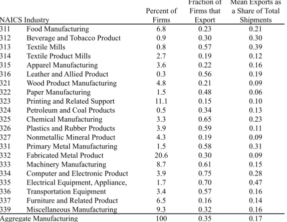
4.1 Firm Exporting Percent of Firms Fraction of Firms that Export Mean Exports as a Share of Total Shipments 311 Food Manufacturing 6.8 0.23 0.21

312 Beverage and Tobacco Product 0.9 0.30 0.30

313 Textile Mills 0.8 0.57 0.39

314 Textile Product Mills 2.7 0.19 0.12

315 Apparel Manufacturing 3.6 0.22 0.16

316 Leather and Allied Product 0.3 0.56 0.19

321 Wood Product Manufacturing 4.8 0.21 0.09

322 Paper Manufacturing 1.5 0.48 0.06

323 Printing and Related Support 11.1 0.15 0.10 324 Petroleum and Coal Products 0.5 0.34 0.13

325 Chemical Manufacturing 3.3 0.65 0.23

326 Plastics and Rubber Products 3.9 0.59 0.11 327 Nonmetallic Mineral Product 4.3 0.19 0.09 331 Primary Metal Manufacturing 1.5 0.58 0.31

332 Fabricated Metal Product 20.6 0.30 0.09

333 Machinery Manufacturing 8.7 0.61 0.15

334 Computer and Electronic Product 3.9 0.75 0.28 335 Electrical Equipment, Appliance, 1.7 0.70 0.47

336 Transportation Equipment 3.4 0.57 0.16

337 Furniture and Related Product 6.5 0.16 0.14 339 Miscellaneous Manufacturing 9.3 0.32 0.16

Aggregate Manufacturing 100 0.35 0.17

NAICS Industry

Notes: Data are from the 2007 U.S. Census of Manufactures. Column 2 summarizes the distribution of manufacturing firms across three-digit NAICS manufacturing industries. Column 3 reports the share of firms in each industry that export. Firm exports measured using customs information from LFTTD. The final column reports mean exports as a percent of total shipments across all firms that export in the noted industry.

Table 1: Firm Exporting

Exporting is a relatively rare firm activity. Of the 5.5 million firms operating in the United States in 2000, just 4 percent engaged in exporting. Even within the smaller set of U.S. firms active in industries

more predisposed to exporting – like those in the manufacturing, mining, or agricultural sectors that produce tradable goods – only 15 percent were exporters.

Table 1provides further evidence on firm export participation using data from the 2007 LFTTD and building on the earlier results from Bernard and Jensen (1995, 1999). Column (1) reports the share of each three-digit North American Industrial Classification (NAIC) industry in the number of manufacturing firms, which ranges from 0.3 percent for Leather and Allied Products (316) to 20.6 percent for Fabricated Metal Products (332).

Column (2) summarizes the share of firms within each industry that export. Consistent with the selection of only some firms into export markets in heterogeneous firm theories, around 35 percent of firms in the U.S. manufacturing sector export. However, this share of exporters ranges rather widely, from 75 percent of firms in Computer and Electronic Products (311) to 15 percent of firms in Printing and Related Support (323). Comparing across the rows of the column, the variation in the share of exporters accords with priors about industries in which the U.S. is likely to have comparative advantage. High-skill and capital-intensive sectors such as Electrical Equipment, Appliance (335) have exporter shares more than twice as large as those of labor-intensive sectors such as Apparel Manufacturing (315). This variation in the share of exporters with industry factor intensity is in line with the predictions of the model of heterogeneous firms and comparative advantage ofBernard, Redding, and Schott(2007). Column (3) presents the average share of exports in firm shipments for each sector. Here again we find evidence of the scarcity of trade. The average export share for manufacturing as a whole of 17 percent is substantially lower than would be predicted in a world of zero trade costs and identical and homothetic preferences.22 Although trade costs directly reduce the share of exports in firm shipments relative to such a frictionless world, other contributory factors are the selection of only a subset of firms into export markets (as inEaton, Kortum, and Kramarz (2011)) and the selection of only a subset of products within firms into export markets (as inBernard, Redding, and Schott(2011)).

We also find substantial variation in the average share of exports in firm shipments across industries, ranging from a high of 47 percent in Electrical Equipment (335) to a low of 6 percent in Paper Manufac-turing (322). Furthermore, this variation again appears related to priors about comparative advantage, with substantially higher export shares in Electrical Equipment, Appliance (335) than in Apparel Man-ufacturing (315). This relationship is consistent with a model in which the selection of heterogeneous firms into export markets and the selection of products within firms into export markets is influenced by comparative advantage, as inBernard, Redding, and Schott(2007,2011).

Comparing the results for 2007 in Table 1with those for 2002 in Bernard, Jensen, Redding, and Schott(2007), we find a larger fraction of exporters and a higher share of firm exports in total shipments in Table 1. The main reason for this difference is that Table 1 measures firm exporting using the

22_{In such a frictionless world, the share of a firm’s exports in its total shipments would equal the share of the rest of the world}

customs records from LFTTD, whereas Bernard, Jensen, Redding, and Schott(2007) measures firm exporting using the export question in the Census of Manufactures.23 Following the 2001 recession and the granting of Permanent Normal Trading Relations (PNTR) to China, there was also a sharp decline in overall employment and high rates of exit in U.S. manufacturing (as examined inPierce and Schott(2012)), both of which are likely to differ between exporters and non-exporters.

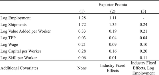
4.2 Exporter Characteristics

Exporters are not only rare but look systematically different from non-exporters. In Table2, we high-light these differences by estimating export premia using the 2007 LFTTD and following the approach ofBernard and Jensen(1995,1999). Each cell in the table corresponds to a separate regression, in which we regress the log of a firm characteristic on a dummy variable for whether a firm exports. Column (1) estimates these regressions for the firm characteristics shown in the rows of the table. Since the depen-dent variables are in logarithms, the estimated coefficients can be interpreted as percentages (up to a log approximation). We find that exporting firms have 128 percent more employment, 172 percent higher shipments, 33 percent higher value-added per worker, and 3 percent higher total factor productivity (TFP).24All of these differences are statistically significant at conventional critical values.25

Column (2) estimates the same regression including industry fixed effects to control for the fact that export participation is correlated with industry characteristics, as discussed in the previous section. We find smaller but still substantial within-industry differences in performance between exporters and non-exporters. Exporters are larger than nonexporters, by approximately 111 percent for employment and 135 percent for shipments; they are more productive by roughly 19 percent for value-added per worker and 4 percent for TFP; they also pay higher wages by around 9 percent. Finally, exporters are relatively more capital- and skill-intensive than nonexporters by approximately 16 and 1 percent, respectively. All of these differences are again statistically significant at conventional critical values. Column (3) shows that the estimated differences are not driven solely by firm size. Including log firm employment as an additional control, we continue to find statistically significant differences between exporters and non-exporters within the same industry for all the other firm characteristics.

23_{Using this alternative definition of firm exporting from the Census of Manufactures, we find a relatively similar pattern}

of results for 2007 as for 2002 inBernard, Jensen, Redding, and Schott(2007). Therefore the customs records from LFTTD imply that exporting is more prevalent than would be concluded based on the export question in the Census of Manufactures.

24_{Total Factor Productivity (TFP) is measured using the Törnqvist superlative index number ofCaves, Christensen, and}

Diewert(1982). Since the differences between exporters and nonexporters are often large, the log approximation can un-derstate considerably the size of these differences. Taking exponents of the employment coefficient in Column 1 of Table2, exporting firms have 260 percent more employment (since 100*(exp(1.28)-1)=260).

25_{Similar performance differences are observed between plants that ship short versus long distances within the U.S., as}

(1) (2) (3)

Log Employment 1.28 1.11

-Log Shipments 1.72 1.35 0.24

Log Value Added per Worker 0.33 0.19 0.21

Log TFP 0.03 0.04 0.04

Log Wage 0.21 0.09 0.10

Log Capital per Worker 0.28 0.16 0.20

Log Skill per Worker 0.06 0.01 0.11

Additional Covariates None Industry Fixed _Effects

Industry Fixed Effects, Log Employment Exporter Premia

Notes: Notes: Data are for 2007 and are from the U.S. Census of Manufactures. All results are from bivariate OLS regressions of firm characteristic in first column on a dummy variable indicating firm's export status. Firm exports mea