These notes are based on a section of a full biophysics course which I teach at Princeton, aimed at PhD students in Physics. In the current organization, this section includes an account of Laughlin’s ideas of optimization in the fly retina, as well as some pointers to topics in the next lecture. Gradually the whole course is being turned into a book, to be published by Princeton University Press. I hope this extract is useful in the context of our short course, and of course I would be grateful for any feedback.
The generation of physicists who turned to biologi-cal phenomena in the wake of quantum mechanics noted that to understand life one has to understand not just the flow of energy (as in inanimate systems) but also the flow of information. There is, of course, some difficulty in translating the colloquial notion of information into something mathematically precise. Indeed, almost all statistical mechanics textbooks note that the entropy of a gas measures our lack of information about the micro-scopic state of the molecules, but often this connection is left a bit vague or qualitative. Shannon proved a theorem that makes the connection precise [Shannon 1948]: en-tropy is the unique measure of available information con-sistent with certain simple and plausible requirements. Further, entropy also answers the practical question of how much space we need to use in writing down a de-scription of the signals or states that we observe. This leads to a notion of efficient representation, and in this section of the course we’ll explore the possibility that bi-ological systems in fact form efficient representations of relevant information.
I. ENTROPY AND INFORMATION
Two friends, Max and Allan, are having a conversa-tion. In the course of the conversation, Max asks Allan what he thinks of the headline story in this morning’s newspaper. We have the clear intuitive notion that Max will ‘gain information’ by hearing the answer to his ques-tion, and we would like to quantify this intuition. Fol-lowing Shannon’s reasoning, we begin by assuming that Max knows Allan very well. Allan speaks very proper English, being careful to follow the grammatical rules even in casual conversation. Since they have had many political discussions Max has a rather good idea about how Allan will react to the latest news. Thus Max can make a list of Allan’s possible responses to his question, and he can assign probabilities to each of the answers. From this list of possibilities and probabilities we can compute an entropy, and this is done in exactly the same way as we compute the entropy of a gas in statistical me-chanics or thermodynamics: If the probability of the nth
possible response ispn, then the entropy is
S =−X
n
pnlog2pnbits. (1)
The entropy S measures Max’s uncertainty about
what Allan will say in response to his question. Once Allan gives his answer, all this uncertainty is removed— one of the responses occurred, corresponding to p= 1, and all the others did not, corresponding to p= 0—so the entropy is reduced to zero. It is appealing to equate this reduction in our uncertainty with the information we gain by hearing Allan’s answer. Shannon proved that this is not just an interesting analogy; it is theonly defi-nition of information that conforms to some simple con-straints.
A. Shannon’s uniqueness theorem
To start, Shannon assumes that the information gained on hearing the answer can be written as a func-tion of the probabilities pn.1 Then if all N possible
an-swers are equally likely the information gained should be a monotonically increasing function ofN. The next con-straint is that if our question consists of two parts, and if these two parts are entirely independent of one another, then we should be able to write the total information gained as the sum of the information gained in response to each of the two subquestions. Finally, more general multipart questions can be thought of as branching trees, where the answer to each successive part of the question provides some further refinement of the probabilities; in this case we should be able to write the total information gained as the weighted sum of the information gained at each branch point. Shannon proved that the only func-tion of the{pn}consistent with these three postulates—
monotonicity, independence, and branching—is the en-tropyS, up to a multiplicative constant.
To prove Shannon’s theorem we start with the case where allNpossible answers are equally likely. Then the information must be a function ofN, and let this func-tion be f(N). Consider the special caseN =km. Then we can think of our answer—one out ofN possibilities— as being given inmindependent parts, and in each part we must be told one of k equally likely possibilities.2
1In particular, this ‘zeroth’ assumption means that we must take seriously the notion of enumerating the possible answers. In this framework we cannot quantify the information that would be gained upon hearing a previously unimaginable answer to our question.
But we have assumed that information from indepen-dent questions and answers must add, so the function f(N) must obey the condition
f(km) =mf(k). (2) It is easy to see that f(N)∝ logN satisfies this equa-tion. To show that this is the unique solution, Shannon considers another pair of integers`andnsuch that
km≤`n≤km+1, (3) or, taking logarithms,
m n ≤ log` logk ≤ m n + 1 n. (4)
Now because the information measuref(N) is monoton-ically increasing withN, the ordering in Eq. (3) means that
f(km)≤f(`n)≤f(km+1), (5) and hence from Eq. (2) we obtain
mf(k)≤nf(`)≤(m+ 1)f(k). (6) Dividing through bynf(k) we have
m n ≤ f(`) f(k) ≤ m n + 1 n, (7)
which is very similar to Eq. (4). The trick is now that with k and ` fixed, we can choose an arbitrarily large value forn, so that 1/n=is as small as we like. Then Eq. (4) is telling us that
m n − log` logk < , (8)
and hence Eq. (7) for the function f(N) can similarly be rewritten as m n − f(`) f(k) < ,or (9) f(`) f(k)− log` logk ≤ 2, (10)
so thatf(N)∝logN as promised.3
We are not quite finished, even with the simple case of N equally likely alternatives, because we still have an arbitrary constant of proportionality. We recall that
place (‘digit’ is the wrong word fork6= 10) number in basek. Themindependent parts of the answer correspond to specifying the number from 0 tok−1 that goes in each of themplaces. 3 If we were allowed to considerf(N) as a continuous function,
then we could make a much simpler argument. But, strictly speaking,f(N) is defined only at integer arguments.
the same issue arises is statistical mechanics: what are the units of entropy? In a physical chemistry course you might learn that entropy is measured in “entropy units,” with the property that if you multiply by the absolute temperature (in Kelvin) you obtain an energy in units of calories per mole; this happens because the constant of proportionality is chosen to be the gas constant R, which refers to Avogadro’s number of molecules.4 In
physics courses entropy is often defined with a factor of Boltzmann’s constant kB, so that if we multiply by the absolute temperature we again obtain an energy (in Joules) but now per molecule (or per degree of freedom), not per mole. In fact many statistical mechanics texts take the sensible view that temperature itself should be measured in energy units—that is, we should always talk about the quantity kBT, not T alone—so that the en-tropy, which after all measures the number of possible states of the system, is dimensionless. Any dimension-less proportionality constant can be absorbed by choos-ing the base that we use for takchoos-ing logarithms, and in information theory it is conventional to choose base two. Finally, then, we have f(N) = log2N. The units of this measure are called bits, and one bit is the information contained in the choice between two equally likely alter-natives.
Ultimately we need to know the information conveyed in the general case where our N possible answers all have unequal probabilities. To make a bridge to this general problem from the simple case of equal probabil-ities, consider the situation where all the probabilities are rational, that is
pn=
kn P
mkm
, (11)
where all the kn are integers. It should be clear that if
we can find the correct information measure for rational {pn}then by continuity we can extrapolate to the general
case; the trick is that we can reduce the case of rational probabilities to the case of equal probabilities. To do this, imagine that we have a total of Ntotal = Pmkm
possible answers, but that we have organized these into N groups, each of which contains kn possibilities. If
we specified the full answer, we would first tell which group it was in, then tell which of the kn possibilities
was realized. In this two step process, at the first step we get the information we are really looking for—which of the N groups are we in—and so the information in
4Whenever I read about entropy units (or calories, for that mat-ter) I imagine that there was some great congress on units at which all such things were supposed to be standardized. Of course every group has its own favorite nonstandard units. Per-haps at the end of some long negotiations the chemists were allowed to keep entropy units in exchange for physicists contin-uing to use electron Volts.
the first step is our unknown function,
I1=I({pn}). (12)
At the second step, if we are in group n then we will gain log2knbits, because this is just the problem of choosing
from kn equally likely possibilities, and since group n
occurs with probability pn the average information we
gain in the second step is I2=
X n
pnlog2kn. (13)
But this two step process is not the only way to compute the information in the enlarged problem, because, by construction, the enlarged problem is just the problem of choosing from Ntotal equally likely possibilities. The
two calculations have to give the same answer, so that I1+I2 = log2(Ntotal), (14) I({pn}) + X n pnlog2kn = log2( X m km). (15)
Rearranging the terms, we find I({pn}) = − X n pnlog2 kn P mkm (16) = −X n pnlog2pn. (17)
Again, although this is worked out explicitly for the case where the pn are rational, it must be the general
an-swer if the information measure is continuous. So we are done: the information obtained on hearing the answer to a question is measured uniquely by the entropy of the distribution of possible answers.
If we phrase the problem of gaining information from hearing the answer to a question, then it is natural to think about a discrete set of possible answers. On the other hand, if we think about gaining information from the acoustic waveform that reaches our ears, then there is a continuum of possibilities. Naively, we are tempted to write
Scontinuum=− Z
dxP(x) log2P(x), (18) or some multidimensional generalization. The difficulty, of course, is that probability distributions for continuous variables [likeP(x) in this equation] have units—the dis-tribution of x has units inverse to the units of x—and we should be worried about taking logs of objects that have dimensions. Notice that if we wanted to compute a difference in entropy between two distributions, this problem would go away. This is a hint that only entropy differences are going to be important.5
5 The problem of defining the entropy for continuous variables is
B. Writing down the answers
In the simple case where we ask a question and there are exactly N = 2m possible answers, all with equal probability, the entropy is just m bits. But if we make a list of all the possible answers we can label each of them with a distinct m–bit binary number: to specify the answer all I need to do is write down this number. Note that the answers themselves can be very complex: different possible answers could correspond to lengthy essays, but the number of pages required to write these essays is irrelevant. If we agree in advance on the set of possible answers, all I have to do in answering the question is to provide a unique label. If we think of the label as a ‘codeword’ for the answer, then in this simple case the length of the codeword that represents the nth possible answer is given by`
n=−log2pn, and
the average length of a codeword is given by the entropy. It will turn out that the equality of the entropy and the average length of codewords is much more general than our simple example. Before proceding, however, it is important to realize that the entropy is emerging as the answer to two very different questions. In the first case we wanted to quantify our intuitive notion of gaining information by hearing the answer to a question. In the second case, we are interested in the problem of representing this answer in the smallest possible space. It is quite remarkable that the only way of quantifying how much we learn by hearing the answer to a question is to measure how much space is required to write down the answer.
Clearly these remarks are interesting only if we can treat more general cases. Let us recall that in statistical mechanics we have the choice of working with a micro-canonical ensemble, in which an ensemble of systems is
familiar in statistical mechanics. In the simple example of an ideal gas in a finite box, we know that the quantum version of the problem has a discrete set of states, so that we can compute the entropy of the gas as a sum over these states. In the limit that the box is large, sums can be approximated as integrals, and if the temperature is high we expect that quantum effects are negligible and one might naively suppose that Planck’s con-stant should disappear from the results; we recall that this is not quite the case. Planck’s constant has units of momentum times position, and so is an elementary area for each pair of conjugate position and momentum variables in the classical phase space; in the classical limit the entropy becomes (roughly) the loga-rithm of the occupied volume in phase space, but this volume is measured in units of Planck’s constant. If we had tried to start with a classical formulation (as did Boltzmann and Gibbs, of course) then we would find ourselves with the problems of Eq. (18), namely that we are trying to take the logarithm of a quantity with dimensions. If we measure phase space volumes in units of Planck’s constant, then all is well. The important point is that the problems with defining a purely classical en-tropy donotstop us from calculating entropy differences, which are observable directly as heat flows, and we shall find a similar situation for the information content of continuous (“classical”) variables.
distributed uniformly over states of fixed energy, or with a canonical ensemble, in which an ensemble of systems is distributed across states of different energies accord-ing to the Boltzmann distribution. The microcanonical ensemble is like our simple example with all answers hav-ing equal probability: entropy really is just the log of the number of possible states. On the other hand, we know that in the thermodynamic limit there is not much differ-ence between the two ensembles. This suggests that we can recover a simple notion of representing answers with codewords of length`n=−log2pnprovided that we can
find a suitbale analog of the thermodynamic limit.
Imagine that instead of asking a question once, we ask it many times. As an example, every day we can ask the weatherman for an estimate of the temperature at noon the next day. Now instead of trying to represent the an-swer to one question we can try to represent the whole stream of answers collected over a long period of time. Thus instead of a possible answer being labelled n, possi-ble sequences of answers are labelled by n1n2· · ·nN. Of course these sequences have probabilitesP(n1n2· · ·nN),
and from these probabilities we can compute an entropy that must depend on the length of the sequence,
S(N) =−X n1 X n2 · · ·X nN P(n1n2· · ·nN) log2P(n1n2· · ·nN). (19)
Notice we are not assuming that successive questions have independent answers, which would correspond to P(n1n2· · ·nN) =Q
N i=1pni.
Now we can draw on our intuition from statistical me-chanics. The entropy is an extensive quantity, which means that as N becomes large the entropy should be proportional toN; more precisely we should have
lim N→∞
S(N)
N =S, (20)
where S is the entropy density for our sequence in the same way that a large volume of material has a well defined entropy per unit volume.
The equivalence of ensembles in the thermodynamic limit means that having unequal probabilities in the Boltzmann distribution has almost no effect on anything we want to calculate. In particular, for the Boltzmann distribution we know that, state by state, the log of the probability is the energy and that this energy is itself an extensive quantity. Further we know that (relative) fluctuations in energy are small. But if energy is log probability, and relative fluctuations in energy are small, this must mean that almost all the states we actually observe have log probabilities which are the same. By analogy, all the long sequences of answers must fall into two groups: those with−log2P ≈NS, and those with P ≈ 0. Now this is all a bit sloppy, but it is the right idea: if we are willing to think about long sequences or streams of data, then the equivalence of ensembles tells us that ‘typical’ sequences are uniformly distributed over N ≈2NS possibilities, and that this appproximation
be-comes more and more accurate as the length N of the sequences becomes large.
The idea of typical sequences, which is the information theoretic version of a thermodynamic limit, is enough to tell us that our simple arguments about representing an-swers by binary numbers ought to work on average for
long sequences of answers. We will have to work sig-nificantly harder to show that this is really the smallest possible representation. An important if obvious conse-quence is that if we have many rather unlikekly answers (rather than fewer more likely answers) then we need more space to write the answers down. More profoundly, this turns out to be true answer by answer: to be sure that long sequences of answers take up as little space as possible, we need to use an average of `n = −log2pn
bits to represent each individual answer n. Thus an-swers which are more surprising require more space to write down.
C. Entropy lost and information gained
Returning to the conversation between Max and Al-lan, we assumed that Max would receive a complete an-swer to his question, and hence that all his uncertainty would be removed. This is an idealization, of course. The more natural description is that, for example, the world can take on many statesW, and by observing data D we learn something but not everything aboutW. Be-fore we make our observations, we know only that states of the world are chosen from some distribution P(W), and this distribution has an entropy S(W). Once we observe some particular datum D, our (hopefully im-proved) knowledge ofW is described by the conditional distributionP(W|D), and this has an entropyS(W|D) that is smaller than S(W) if we have reduced our un-certainty about the state of the world by virtue of our observations. We identify this reduction in entropy as the information that we have gained aboutW.
Perhaps this is the point to note that a single observa-tionD is not, in fact, guaranteed to provide positive in-formation [see, for example, DeWeese and Meister 1999]. Consider, for instance, data which tell us that all of our
previous measurements have larger error bars than we thought: clearly such data, at an intuitive level, reduce our knowledge about the world and should be associ-ated with a negative information. Another way to say this is that some data pointsD will increase our uncer-tainty about state W of the world, and hence for these particular data the conditional distributionP(W|D) has a larger entropy than the prior distribution P(D). If we identify information with the reduction in entropy,
ID=S(W)−S(W|D), then such data points are associ-ated unambiguously with negative information. On the other hand, we might hope that, on average, gathering data corresponds to gaining information: although sin-gle data points can increase our uncertainty, the average over all data points does not.
If we average over all possible data—weighted, of course, by their probability of occurrenceP(D)—we ob-tain the average information that D provides aboutW:
I(D→W) = S(W)−X D P(D)S(W|D) (21) = −X W P(W) log2P(W)− X D P(D) " −X W P(W|D) log2P(W|D) # (22) = −X W X D P(W, D) log2P(W) + X W X D P(W|D)P(D) log2P(W|D) (23) = −X W X D P(W, D) log2P(W) + X W X D P(W, D) log2P(W|D) (24) = X W X D P(W, D) log2 P(W|D) P(W) (25) = X W X D P(W, D) log2 P(W, D) P(W)P(D) . (26)
We see that, after all the dust settles, the information which D provides about W is symmetric in D and W. This means that we can also view the state of the world as providing information about the data we will observe, and this information is, on average, the same as the data will provide about the state of the world. This ‘informa-tion provided’ is therefore often called the mutual in-formation, and this symmetry will be very important in subsequent discussions; to remind ourselves of this sym-metry we writeI(D;W) rather thanI(D→W).
One consequence of the symmetry or mutuality of in-formation is that we can write
I(D;W) = S(W)−X D P(D)S(W|D) (27) = S(D)−X W P(W)S(D|W). (28)
If we consider only discrete sets of possibilities then en-tropies are positive (or zero), so that these equations imply
I(D;W) ≤ S(W) (29) I(D;W) ≤ S(D). (30) The first equation tells us that by observing D we can-not learn more about the world then there is entropy in the world itself. This makes sense: entropy measures
the number of possible states that the world can be in, and we cannot learn more than we would learn by re-ducing this set of possibilities down to one unique state. Although sensible (and, of course, true), this is not a terribly powerful statement: seldom are we in the po-sition that our ability to gain knowledge is limited by the lack of possibilities in the world around us.6 The second equation, however, is much more powerful. It says that, whatever may be happening in the world, we can never learn more than the entropy of the distribu-tion that characterizes our data. Thus, if we ask how much we can learn about the world by taking readings from a wind detector on top of the roof, we can place a bound on the amount we learn just by taking a very long stream of data, using these data to estimate the distribution P(D), and then computing the entropy of this distribution.
The entropy of our observations7thus limits how much
6This is not quite true. There is a tradition of studying the ner-vous system as it responds to highly simplified signals, and under these conditions the lack of possibilities in the world can be a sig-nificant limitation, substantially confounding the interpretation of experiments.
7In the same way that we speak about the entropy of a gas I will often speak about the entropy of a variable or the entropy of a
we can learn no matter what question we were hoping to answer, and so we can think of the entropy as setting (in a slight abuse of terminology) the capacity of the data D to provide or to convey information. As an example, the entropy of neural responses sets a limit to how much information a neuron can provide about the world, and we can estimate this limit even if we don’t yet understand what it is that the neuron is telling us (or the rest of the brain).
D. Optimizing input/output relations
These ideas are enough to get started on “designing” some simple neural processes [Laughlin 1981]. Imagine that a neuron is responsible for representing a single number such as the light intensity I averaged over a small patch of the retina (don’t worry about time depen-dence). Assume that this signal will be represented by a continuous voltageV, which is true for the first stages of processing in vision, as we have seen in the first section of the course. The information that the voltage provides about the intensity is
I(V → I) = Z dI Z dV P(V,I) log2 P(V,I) P(V)P(I) (31) = Z dI Z dV P(V,I) log2 P(V|I) P(V) . (32) The conditional distribution P(V|I) describes the pro-cess by which the neuron responds to its input, and so this is what we should try to “design.”
Let us suppose that the voltage is on average a non-linear function of the intensity, and that the dominant source of noise is additive (to the voltage), independent of light intensity, and small compared with the overall dynamic range of the cell:
V =g(I) +ξ, (33) with some distributionPnoise(ξ) for the noise. Then the
conditional distribution
P(V|I) =Pnoise(V −g(I)), (34)
and the entropy of this conditional distribution can be written as
Scond = − Z
dV P(V|I) log2P(V|I) (35)
response. In the gas, we understand from statistical mechanics that the entropy is defined not as a property of the gas but as a property of the distribution or ensemble from which the mi-croscopic states of the gas are chosen; similarly we should really speak here about “the entropy of the distribution of observa-tions,” but this is a bit cumbersome. I hope that the slightly sloppy but more compact phrasing does not cause confusion.
= −
Z
dξ Pnoise(ξ) log2Pnoise(ξ). (36)
Note that this is a constant, independent both of the light intensity and of the nonlinear input/output relation g(I). This is useful because we can write the information as a difference between the total entropy of the output variable V and this conditional or noise entropy, as in Eq. (28):
I(V → I) =−
Z
dV P(V) log2P(V)−Scond. (37)
With Scond constant independent of our ‘design,’
max-imizing information is the same as maxmax-imizing the en-tropy of the distribution of output voltages. Assuming that there are maximum and minimum values for this voltage, but no other constraints, then the maximum en-tropy distribution is just the uniform distribution within the allowed dynamic range. But if the noise is small it doesn’t contribute much to broadeningP(V) and we cal-culate this distribution as if there were no noise, so that P(V)dV = P(I)dI, (38)
dV dI =
1
P(V)·P(I). (39) Since we want to haveV =g(I) andP(V) = 1/(Vmax−
Vmin), we find
dg(I)
dI = (Vmax−Vmin)P(I), (40) g(I) = (Vmax−Vmin)
Z I
Imin
dI0P(I0). (41)
Thus, the optimal input/output relation is proportional to the cumulative probability distribution of the input signals.
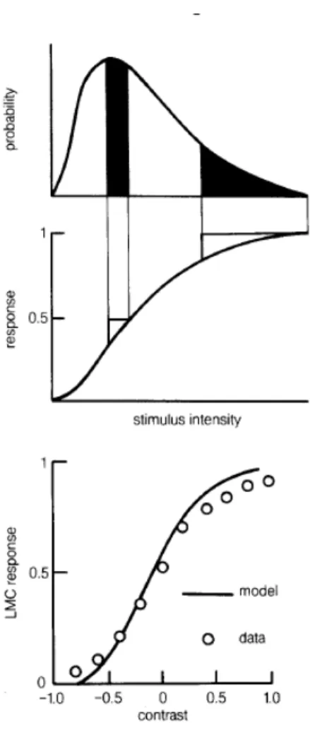
The predictions of Eq. (41) are quite interesting. First of all it makes clear that any theory of the nervous sys-tem which involves optimizing information transmission or efficiency of representation inevitably predicts that the computations done by the nervous system must be matched to the statistics of sensory inputs (and, presum-ably, to the statistics of motor outputs as well). Here the matching is simple: in the right units we could just read off the distribution of inputs by looking at the (differ-entiated) input/output relation of the neuron. Second, this simple model automatically carries some predictions about adaptation to overall light levels. If we live in a world with diffuse light sources that are not directly vis-ible, then the intensity which reaches us at a point is the product of the effective brightness of the source and some local reflectances. As is it gets dark outside the re-flectances don’t change—these are material properties— and so we expect that the distribution P(I) will look the same except for scaling. Equivalently, if we view the input as the log of the intensity, then to a good approx-imationP(logI) just shifts linearly along the logI axis
FIG. 1 Matching of input/output relation to the distribu-tion of inputs in the fly large monopolar cells (LMCs). Top, a schematic probability distribution for light intensity. Mid-dle, the optimal input/output relation according to Eq (41), highlighting the fact that equal ranges of output correspond to equal mass under the input distribution. Bottom, mea-surements of the input/output relation in LMCs compared with these predictions From [Laughlin 1981 & 1987].
as mean light intensity goes up and down. But then the optimal input/output relationg(I) would exhibit a similar invariant shape with shifts along the input axis when expressed as a function of logI, and this is in rough agreement with experiments on light/dark adaptation in a wide variety of visual neurons. Finally, although obvi-ously a simplified version of the real problem facing even the first stages of visual processing, this calculation does make a quantitative prediction that would be tested if we measure both the input/output relations of early vi-sual neurons and the distribution of light intensities that the animal encounters in nature.
Laughlin made this comparison (25 years ago!) for
the fly visual system [Laughlin 1981]. He built an elec-tronic photodetector with aperture and spectral sensi-tivity matched to those of the fly retina and used his photodetector to scan natural scenes, measuring P(I) as it would appear at the input to these neurons. In parallel he characterized the second order neurons of the fly visual system—the large monopolar cells which re-ceive direct synaptic input from the photoreceptors—by measuring the peak voltage response to flashes of light. The agreement with Eq. (41) was remarkable (Fig 1), especially when we remember that there are no free pa-rameters. While there are obvious open questions (what happened to time dependence?), this is a really beautiful result that inspires us to take these ideas more seriously.
E. Maximum entropy distributions
Since the information we can gain is limited by the entropy, it is natural to ask if we can put limits on the entropy using some low order statistical properties of the data: the mean, the variance, perhaps higher moments or correlation functions, ... . In particular, if we can say that the entropy has a maximum value consistent with the observed statistics, then we have placed a firm upper bound on the information that these data can convey.
The problem of finding the maximum entropy given some constraint again is familiar from statistical mechan-ics: the Boltzmann distribution is the distribution that has the largest possible entropy given the mean energy. More generally, imagine that we have knowledge not of the whole probability distributionP(D) but only of some expectation values,
hfii= X
D
P(D)fi(D), (42)
where we allow that there may be several expectation values known (i = 1,2, ..., K). Actually there is one more expectation value that we always know, and this is that the average value of one is one; the distribution is nor-malized:
hf0i= X
D
P(D) = 1. (43)
Given the set of numbers {hf0i,hf1i,· · ·,hfKi} as con-straints on the probability distributionP(D), we would like to know the largest possible value for the entropy, and we would like to find explicitly the distribution that provides this maximum.
The problem of maximizing a quantity subject to con-straints is formulated using Lagrange multipliers. In this case, we want to maximizeS =−P
P(D) log2P(D), so
we introduce a function ˜S, with one Lagrange multiplier λi for each constraint:
˜ S[P(D)] = −X D P(D) log2P(D)− K X i=0 λihfii (44) = − 1 ln 2 X D P(D) lnP(D)− K X i=0 λi X D P(D)fi(D). (45)
Our problem is then to find the maximum of the function ˜
S, but this is easy because the probability for each value ofD appears independently. The result is that
P(D) = 1 Z exp " − K X i=1 λifi(D) # , (46)
whereZ = exp(1 +λ0) is a normalization constant.
There are few more things worth saying about maxi-mum entropy distributions. First, we recall that if the value ofDindexes the states n of a physical system, and we know only the expectation value of the energy,
hEi=X
n
PnEn, (47)
then the maximum entropy distribution is Pn=
1
Z exp(−λEn), (48) which is the Boltzmann distribution (as promised). In this case the Lagrange multiplier λ has physical meaning—it is the inverse temperature. Further, the function ˜Sthat we introduced for convenience is the dif-ference between the entropy and λ times the energy; if we divide through by λand flip the sign, then we have the energy minus the temperature times the entropy, or the free energy. Thus the distribution which maximizes entropy at fixed average energy is also the distribution which minimizes the free energy.
If we are looking at a magnetic system, for example, and we know not just the average energy but also the average magnetization, then a new term appears in the exponential of the probability distribution, and we can interpret this term as the magnetic field multiplied by the magnetization. More generally, for every order pa-rameter which we assume is known, the probability dis-tribution acquires a term that adds to the energy and
can be thought of as a product of the order parameter with its conjugate force. Again, all these remarks should be familiar from a statistical mechanics course.
Probability distributions that have the maximum en-tropy form of Eq. (46) are special not only because of their connection to statistical mechanics, but because they form what the statisticians call an ‘exponential fam-ily,’ which seems like an obvious name. The important point is that exponential families of distributions are (almost) unique in having sufficient statistics. To un-derstand what this means, consider the following prob-lem: We observe a set of samples D1, D2,· · ·, DN, each of which is drawn independently and at random from a distributionP(D|{λi}). Assume that we know the form
of this distribution but not the values of the parameters {λi}. How can we estimate these parameters from the
set of observations{Dn}? Notice that our data set{Dn}
consists ofN numbers, andN can be very large; on the other hand there typically are a small number K N of parametersλi that we want to estimate. Even in this
limit, no finite amount of data will tell us the exact val-ues of the parameters, and so we need a probabilistic formulation: we want to compute the distribution of pa-rameters given the data,P({λi}|{Dn}). We do this using
Bayes’ rule, P({λi}|{Dn}) =
1 P({Dn})
·P({Dn}|{λi})P({λi}), (49)
where P({λi}) is the distribution from which the
pa-rameter values themselves are drawn. Then since each datum Dnis drawn independently, we have
P({Dn}|{λi}) =
N
Y
n=1
P(Dn|{λi}). (50)
For probability distributions of the maximum entropy form we can proceed further, using Eq. (46):
P({λi}|{Dn}) = 1 P({Dn}) ·P({Dn}|{λi})P({λi}) = P({λi}) P({Dn}) N Y n=1 P(Dn|{λi}) (51)
= P({λi}) ZNP({D n}) N Y n=1 exp " − K X i=1 λifi(Dn) # (52) = P({λi}) ZNP({D n}) exp " −N K X i=1 λi 1 N N X n=1 fi(Dn) # . (53)
We see that allof the information that the data points {Dn} can give about the parametersλi is contained in
the average values of the functionsfi over the data set, or the ‘empirical means’ ¯fi,
¯ fi = 1 N N X n=1 fi(Dn). (54)
More precisely, the distribution of possible parameter values consistent with the data depends not on all details of the data, but rather only on the empirical means{f¯i},
P({λi}|D1, D2,· · ·, DN) =P({λi}|{f¯j}), (55)
and a consequence of this is the information theoretic statement
I(D1, D2,· · ·, DN → {λi}) =I({f¯j} → {λi}). (56)
This situation is described by saying that the reduced set of variables{f¯j}constitutesufficient statisticsfor
learn-ing the distribution. Thus, for distributions of this form, the problem of compressingN data points intoK << N variables that are relevant for parameter estimation can be solved explicitly: if we keep track of the running aver-ages ¯fiwe can compress our data as we go along, and we
are guaranteed that we will never need to go back and examine the data in more detail. A clear example is that if we know data are drawn from a Gaussian distribution, running estimates of the mean and variance contain all the information available about the underlying parame-ter values.
The Gaussian example makes it seem that the con-cept of sufficient statistics is trivial: of course if we know that data are chosen from a Gaussian distribution, then to identify the distribution all we need to do is to keep track of two moments. Far from trivial, this situation is quite unusual. Most of the distributions that we might write down do not have this property—even if they are described by a finite number of parameters, we cannot guarantee that a comparably small set of empirical ex-pectation values captures all the information about the parameter values. If we insist further that the sufficient statistics be additive and permutation symmetric,8then
8 These conditions mean that the sufficient statistics can be con-structed as running averages, and that the same data points in different sequence carry the same information.
it is a theorem that onlyexponential families have suffi-cient statistics.
The generic problem of information processing, by the brain or by a machine, is that we are faced with a huge quantity of data and must extract those pieces that are of interest to us. The idea of sufficient statistics is in-triguing in part because it provides an example where this problem of ‘extracting interesting information’ can be solved completely: if the points D1, D2,· · ·, DN are chosen independently and at random from some distri-bution, the only thing which could possibly be ‘interest-ing’ is the structure of the distribution itself (everything else is random, by construction), this structure is de-scribed by a finite number of parameters, and there is an explicit algorithm for compressing theN data points {Dn}intoKnumbers that preserve all of the interesting
information.9 The crucial point is that this procedure
cannot exist in general, but only for certain classes of probability distributions. This is an introduction to the idea some kinds of structure in data are learnable from random examples, while other structures are not.
Consider the (Boltzmann) probability distribution for the states of a system in thermal equilibrium. If we ex-pand the Hamiltonian as a sum of terms (operators) then the family of possible probability distributions is an ex-ponential family in which the coupling constants for each operator are the parameters analogous to the λi above.
In principle there could be an infinite number of these operators, but for a given class of systems we usually find that only a finite set are “relevant” in the renor-malization group sense: if we write an effective Hamil-tonian for coarse grained degrees of freedom, then only a finite number of terms will survive the coarse graining procedure. If we have only a finite number of terms in the Hamiltonian, then the family of Boltzmann distribu-tions has sufficient statistics, which are just the expec-tation values of the relevant operators. This means that the expectation values of the relevant operators carry all the information that the (coarse grained) configuration of the system can provide about the coupling constants, which in turn is information about the identity or mi-croscopic structure of the system. Thus the statement that there are only a finite number of relevant operators
9There are more subtle questions: How many bits are we squeez-ing out in this process of compression, and how many bits of relevance are left? We return to this and related questions when we talk about learning later in the course.
is also the statement that a finite number of expectation values carries all the information about the microscopic dynamics. The ‘if’ part of this statement is obvious: if there are only a finite number of relevant operators, then the expectation values of these operators carry all the information about the identity of the system. The statisticians, through the theorem about the uniqueness of exponential families, give us the ‘only if’: a finite num-ber of expectation values (or correlation functions) can provide all the information about the systemonly ifthe effective Hamiltonian has a finite number of relevant op-erators. I suspect that there is more to say along these lines, but let us turn instead to some examples.
Consider the situation in which the data D are real numbers x. Suppose that we know the mean value ofx and its variance. This is equivalent to knowledge of two expectation values, ¯ f1 = hxi= Z dxP(x)x, and (57) ¯ f2 = hx2i= Z dxP(x)x2, (58) so we have f1(x) =xand f2(x) = x2. Thus, from Eq.
(46), the maximum entropy distribution is of the form P(x) = 1
Zexp(−λ1x−λ2x
2
). (59) This is a funny way of writing a more familiar ob-ject. If we identify the parameters λ2 = 1/(2σ2) and
λ1 = −hxi/σ2, then we can rewrite the maximum
en-tropy distribution as the usual Gaussian, P(x) = √ 1 2πσ2exp − 1 2σ2(x− hxi) 2 . (60) We recall that Gaussian distributions usually arise through the central limit theorem: if the random vari-ables of interest can be thought of as sums of many inde-pendent events, then the distributions of the observable variables converge to Gaussians. This provides us with a ‘mechanistic’ or reductionist view of why Gaussians are so important. A very different view comes from in-formation theory: if all we know about a variable is the mean and the variance, then the Gaussian distribution is the maximum entropy distribution consistent with this knowledge. Since the entropy measures (returning to our physical intuition) the randomness or disorder of the sys-tem, the Gaussian distribution describes the ‘most ran-dom’ or ‘least structured’ distribution that can generate the known mean and variance.
A somewhat different situation is when the data D are generated by counting. Then the relevant variable is an integer n= 0,1,2,· · ·, and it is natural to imagine that what we know is the mean counthni. One way this problem can arise is that we are trying to communicate and are restricted to sending discrete or quantized units. An obvious case is in optical communication, where the
quanta are photons. In the brain, quantization abounds: most neurons do not generate continuous analog volt-ages but rather communicate with one another through stereotyped pulses or spikes, and even if the voltages vary continuously transmission across a synapse involves the release of a chemical transmitter which is packaged into discrete vesicles. It can be relatively easy to measure the mean rate at which discrete events are counted, and we might want to know what bounds this mean rate places on the ability of the cells to convey information. Alter-natively, there is an energetic cost associated with these discrete events—generating the electrical currents that underlie the spike, constructing and filling the vesicles, ... —and we might want to characterize the mechanisms by their cost per bit rather than their cost per event. If we know the mean count, there is (as for the Boltz-mann distribution) only one functionf1(n) =nthat can
appear in the exponential of the distribution, so that P(n) = 1
Z exp(−λn). (61) Of course we have to choose the Lagrange multiplier to fix the mean count, and it turns out that λ = ln(1 + 1/hni); further we can find the entropy
Smax(counting) = log2(1 +hni) +hnilog2(1 + 1/hni).
(62) The information conveyed by counting something can never exceed the entropy of the distribution of counts, and if we know the mean count then the entropy can never exceed the bound in Eq. (62). Thus, if we have a system in which information is conveyed by counting discrete events, the simple fact that we count only a lim-ited number of events (on average) sets a bound on how much information can be transmitted. We will see that real neurons and synapses approach this fundamental limit.
One might suppose that if information is coded in the counting of discrete events, then each event carries a certain amount of information. In fact this is not quite right. In particular, if we count a large number of events then the maximum counting entropy becomes
Smax(counting;hni → ∞)∼log2(hnie), (63)
and so we are guaranteed that the entropy (and hence the information) per event goes to zero, although the approach is slow. On the other hand, if events are very rare, so that the mean count is much less than one, we find the maximum entropy per event
1
hniSmax(counting;hni<<1)∼log2
e hni
, (64) which is arbitrarily large for small mean count. This makes sense: rare events have an arbitrarily large ca-pacity to surprise us and hence to convey information. It is important to note, though, that the maximum en-tropy per event is a monotonically decreasing function of
the mean count. Thus if we are counting spikes from a neuron, counting in larger windows (hence larger mean counts) is always less efficient in terms of bits per spike. If it is more efficient to count in small time windows, perhaps we should think not about counting but about measuring the arrival times of the discrete events. If we look at a total (large) time interval 0< t < T, then we will observe arrival times t1, t2,· · ·, tN in this interval; note that the number of eventsN is also a random vari-able. We want to find the distributionP(t1, t2,· · ·, tN) that maximizes the entropy while holding fixed the aver-age event rate. We can write the entropy of the distribu-tion as a sum of two terms, one from the entropy of the arrival times given the count and one from the entropy
of the counting distribution:
S ≡ − ∞ X N=0 Z dNtnP(t1, t2,· · ·, tN) log2P(t1, t2,· · ·, tN) = ∞ X N=0 P(N)Stime(N)− ∞ X N=0 P(N) log2P(N), (65)
where we have made use of
P(t1, t2,· · ·, tN) =P(t1, t2,· · ·, tN|N)P(N), (66) and the (conditional) entropy of the arrival times in given by
Stime(N) =− Z
dNtnP(t1, t2,· · ·, tN|N) log2P(t1, t2,· · ·, tN|N). (67)
If all we fix is the mean count, hNi = P
NP(N)N, then the conditional distributions for the locations of the events given the total number of events, P(t1, t2,· · ·, tN|N), are unconstrained. We can maxi-mize the contribution of each of these terms to the en-tropy [the terms in the first sum of Eq. (65)] by making the distributions P(t1, t2,· · ·, tN|N) uniform, but it is important to be careful about normalization. When we integrate over all the timest1, t2,· · ·, tN, we are forget-ting that the events are all identical, and hence that per-mutations of the times describe the same events. Thus the normalization condition isnot
Z T 0 dt1 Z T 0 dt2· · · Z T 0 dtNP(t1, t2,· · ·, tN|N) = 1, (68) but rather 1 N! Z T 0 dt1 Z T 0 dt2· · · Z T 0 dtNP(t1, t2,· · ·, tN|N) = 1. (69)
This means that the uniform distribution must be
P(t1, t2,· · ·, tN|N) = N!
TN, (70)
and hence that the entropy [substituting into Eq. (65)] becomes S =− ∞ X N=0 P(N) log2 N! TN + log2P(N) . (71)
Now to find the maximum entropy we proceed as before. We introduce Lagrange multipliers to constrain the mean count and the normalization of the distribution P(N), which leads to the function
˜ S =− ∞ X N=0 P(N) log2 N! TN + log2P(N) +λ0+λ1N , (72)
and then we maximize this function by varyingP(N). As before the differentNs are not coupled, so the optimization conditions are simple:
0 = ∂ ˜ S ∂P(N) (73) = − 1 ln 2 ln N! TN + lnP(N) + 1 −λ0−λ1N, (74)
lnP(N) = −ln N! TN −(λ1ln 2)N−(1 +λ0ln 2). (75)
Combining terms and simplifying, we have P(N) = 1 Z (λT)N N! , (76) Z = ∞ X N=0 (λT)N N! = exp(λT). (77) This is the Poisson distribution.
The Poisson distribution usually is derived (as in our discussion of photon counting) by assuming that the probability of occurrence of an event in any small time bin of size ∆τ is independent of events in any other bin, and then we let ∆τ→0 to obtain a distribution in the continuum. This is not surprising: we have found that the maximum entropy distribution of events given the mean number of events (or their densityhNi/T) is given by the Poisson distribution, which corresponds to the events being thrown down at random with some proba-bility per unit time (again, hNi/T) and no interactions among the events. This describes an ‘ideal gas’ of events along a line (time). More generally, the ideal gas is the gas with maximum entropy given its density; interac-tions among the gas molecules always reduce the entropy if we hold the density fixed.
If we have multiple variables,x1, x2,· · ·, xN, then we can go through all of the same analyses as before. In par-ticular, if these are continuous variables and we are told the means and covariances among the variables, then the maximum entropy distribution is again a Gaussian distribution, this time the appropriate multidimensional Gaussian. This example, like the other examples so far, is simple in that we can give not only the form of the distribution but we can find the values of the parameters that will satisfy the constraints. In general this is not so easy: think of the Boltzmann distribution, where we would have to adjust the temperature to obtain a given value of the average energy, but if we can give an explicit relation between the temperature and average energy for any system then we have solved almost all of statistical mechanics!
One important example is provided by binary strings. If we label 1s by spin up and 0s by spin down, the bi-nary string is equivalent to an Ising chain {σi}. Fixing
the probability of a 1 is the same as fixing the mean magnetization hσii. If, in addition, we specify the joint
probability of two 1s occurring in bins separated by n steps (for all n), this is equivalent to fixing the spin– spin correlation function hσiσji. The maximum entropy
distribution consistent with these constraints is an Ising model, P[{σi}] = 1 Z exp −h X i σi− X ij Jijσiσj ; (78)
note that the interactions are pairwise (because we fix only a two–point function) but not limited to near neigh-bors. Obviously the problem of finding the exchange in-teractions which match the correlation function is not so simple.
Another interesting feature of the Ising or binary string problem concerns higher order correlation func-tions. If we have continuous variables and constrain the two–point correlation functions, then the maximum en-tropy distribution is Gaussian and there are no nontrivial higher order correlations. But if the signals we observe are discrete, as in the sequence of spikes from a neuron, then the maximum entropy distribution is an Ising model and this model makes nontrivial predictions about the multipoint correlations. In particular, if we record the spike trains fromKseparate neurons and measure all of the pairwise correlation functions, then the correspond-ing Iscorrespond-ing model predicts that there will be irreducible correlations among triplets of neurons, and higher order correlations as well [Schneidman et al 2006].
Before closing the discussion of maximum entropy dis-tributions, note that our simple solution to the problem, Eq. (46), might not work. Taking derivatives and setting them to zero works only if the solution to our problem is in the interior of the domain allowed by the constraints. It is also possible that the solution lies at the boundary of this allowed region. This seems especially likely when we combine different kinds of constraints, such as trying to find the maximum entropy distribution of images con-sistent both with the two–point correlation function and with the histogram of intensity values at one point. The relevant distribution is a 2D field theory with a (gener-ally nonlocal) quadratic ‘kinetic energy’ and some arbi-trary local potential; it is not clear that all combinations of correlations and histograms can be realized, nor that the resulting field theory will be stable under renormal-ization.10 There are many open questions here.
F. Information transmission with noise
We now want to look at information transmission in the presence of noise, connecting back a bit to what we discussed in earlier parts of the of course. Imagine that we are interested in some signalx, and we have a detector that generates data y which is linearly related to the signal but corrupted by added noise:
y=gx+ξ. (79)
10The empirical histograms of local quantities in natural images arestable under renormalization [Ruderman and Bialek 1994].
It seems reasonable in many systems to assume that the noise arises from many added sources (e.g., the Brow-nian motion of electrons in a circuit) and hence has a Gaussian distribution because of the central limit theo-rem. We will also start with the assumption that x is drawn from a Gaussian distribution just because this is a simple place to start; we will see that we can use the maximum entropy property of Gaussians to make some more general statements based on this simple example. The question, then, is how much information observa-tions ony provide about the signalx.
Let us formalize our assumptions. The statement that ξ is Gaussian noise means that once we know x, y is Gaussian distributed around a mean value ofgx:
P(y|x) = p 1 2πhξ2iexp − 1 2hξ2i(y−gx) 2 . (80)
Our simplification is that the signalxalso is drawn from a Gaussian distribution, P(x) = p 1 2πhx2iexp − 1 2hx2ix 2 , (81)
and hencey itself is Gaussian,
P(y) = p 1 2πhy2iexp − 1 2hy2iy 2 (82) hy2i = g2hx2i+hξ2i. (83)
To compute the information thatyprovides aboutxwe use Eq. (26): I(y→x) = Z dy Z dxP(x, y) log2 P(x, y) P(x)P(y) bits (84) = 1 ln 2 Z dy Z dxP(x, y) ln P(y|x) P(y) (85) = 1 ln 2 * ln " p 2πhy2i p 2πhξ2i # − 1 2hξ2i(y−gx) 2+ 1 2hy2iy 2 + , (86)
where byh· · ·iwe understand an expectation value over the joint distributionP(x, y). Now in Eq. (86) we can see that the first term is the expectation value of a con-stant, which is just the constant. The third term involves the expectation value of y2 divided by hy2i, so we can
cancel numerator and denominator. In the second term, we can take the expectation value first ofy withxfixed, and then average over x, but since y =gx+ξ the nu-merator is just the mean square fluctuation ofy around its mean value, which again cancels with thehξ2iin the
denominator. So we have, putting the three terms to-gether, I(y→x) = 1 ln 2 " ln s hy2i hξ2i− 1 2+ 1 2 # (87) = 1 2log2 hy2i hξ2i (88) = 1 2log2 1 +g 2hx2i hξ2i bits. (89)
Although it may seem like useless algebra, I would like to rewrite this result a little bit. Rather than thinking of our detector as adding noise after generating the signal gx, we can think of it as adding noise directly to the
input, and then transducing this corrupted input: y=g(x+ηeff), (90)
where, obviously, ηeff = ξ/g. Note that the “effective
noise” ηeff is in the same units as the input x; this is
called ‘referring the noise to the input’ and is a standard way of characterizing detectors, amplifiers and other de-vices. Clearly if we build a photodetector it is not so useful to quote the noise level in Volts at the output ... we want to know how this noise limits our ability to detect dim lights. Similarly, when we characterize a neuron that uses a stream of pulses to encode a con-tinuous signal, we don’t want to know the variance in the pulse rate; we want to know how noise in the neural response limits precision in estimating the real signal, and this amounts to defining an effective noise level in the units of the signal itself. In the present case this is just a matter of dividing, but generally it is a more com-plex task. With the effective noise level, the information transmission takes a simple form,
I(y→x) =1 2log2 1 + hx 2i hη2 effi bits, (91) or I(y→x) = 1 2log2(1 +SN R), (92)
where the signal to noise ratio is the ratio of the vari-ance in the signal to the varivari-ance of the effective noise, SN R=hx2i/hη2
effi.
The result in Eq. (92) is easy to picture: When we start, the signal is spread over a rangeδx0∼ hx2i1/2, but
by observing the output of our detector we can localize the signal to a small rangeδx1∼ hηeff2 i1/2, and the
reduc-tion in entropy is∼log2(δx0/δx1)∼(1/2)·log2(SN R),
which is approximately the information gain.
As a next step consider the case where we ob-serve several variables y1, y2,· · ·, yK in the hopes of learning about the same number of underlying signals x1, x2,· · ·, xK. The equations analogous to Eq. (79) are
then
yi=gijxj+ξi, (93)
with the usual convention that we sum over repeated indices. The Gaussian assumptions are that eachxi and
ξi has zero mean, but in general we have to think about
arbitrary covariance matrices,
Sij = hxixji (94)
Nij = hξiξji. (95)
The relevant probability distributions are
P({xi}) = 1 p (2π)KdetSexp −1 2xi·(S −1) ij·xj (96) P({yi}|{xi}) = 1 p (2π)KdetN exp −1 2(yj−gikxk)·(N −1) ij·(yj−gjmxm) , (97)
where again the summation convention is used; detS denotes the determinant of the matrixS, and (S−1)
ij is
the ij element in the inverse of the matrixS.
To compute the mutual information we proceed as be-fore. First we find P({yi}) by doing the integrals over
thexi,
P({yi}) = Z
dKxP({yi}|{xi})P({xi}), (98)
and then we write the information as an expectation value, I({yi} → {xi}) = * log2 P ({yi}|{xi}) P({yi}) + , (99)
where h· · ·i denotes an average over the joint distribu-tion P({yi},{xi}). As in Eq. (86), the logarithm can
be broken into several terms such that the expectation value of each one is relatively easy to calculate. Two of three terms cancel, and the one which survives is related to the normalization factors that come in front of the exponentials. After the dust settles we find
I({yi} → {xi}) =
1
2Tr log2[1+N
−1
·(g·S·gT)], (100)
where Tr denotes the trace of a matrix, 1 is the unit matrix, andgT is the transpose of the matrixg.
The matrixg·S·gT describes the covariance of those components of y that are contributed by the signal x. We can always rotate our coordinate system on the space of ys to make this matrix diagonal, which corresponds to finding the eigenvectors and eigenvalues of the covari-ance matrix; these eigenvectors are also called “principal
components.” The eigenvectors describe directions in the space of y which are fluctuating independently, and the eigenvalues are the variances along each of these di-rections. If the covariance of the noise is diagonal in the same coordinate system, then the matrixN−1·(g·S·gT) is diagonal and the elements along the diagonal are the signal to noise ratios along each independent direction. Taking the Tr log is equivalent to computing the infor-mation transmission along each direction using Eq. (92), and then summing the results.
An important case is when the different variables xi
represent a signal sampled at several different points in time. Then there is some underlying continuous func-tion x(t), and in place of the discrete Eq. (93) we have the continuous linear response of the detector to input signals,
y(t) =
Z
dt0M(t−t0)x(t0) +ξ(t). (101)
In this continuous case the analog of the covariance ma-trix hxixji is the correlation function hx(t)x(t0)i. We
are usually interested in signals (and noise) that are sta-tionary. This means that all statistical properties of the signal are invariant to translations in time: a particular pattern of wiggles in the functionx(t) is equally likely to occur at any time. Thus, the correlation function which could in principle depend on two times tandt0 depends only on the time difference,
hx(t)x(t0)i=Cx(t−t0). (102) The correlation function generalizes the covariance ma-trix to continuous time, but we have seen that it can be useful to diagonalize the covariance matrix, thus finding
a coordinate system in which fluctuations in the differ-ent directions are independdiffer-ent. From previous lectures we know that the answer is to go into a Fourier repre-sentation, where (in the Gaussian case) different Fourier components are independent and their variances are (up to normalization) the power spectra.
To complete the analysis of the continuous time Gaus-sian channel described by Eq. (101), we again refer noise to the input by writing
y(t) =
Z
dt0M(t−t0)[x(t0) +ηeff(t0)]. (103)
If both signal and effective noise are stationary, then each has a power spectrum; let us denote the power spectrum of the effective noiseηeff byNeff(ω) and the power
spec-trum ofxbySx(ω) as usual. There is a signal to noise ratio at each frequency,
SN R(ω) = Sx(ω) Neff(ω)
, (104)
and since we have diagonalized the problem by Fourier transforming, we can compute the information just by adding the contributions from each frequency compo-nent, so that I[y(t)→x(t)] = 1 2 X ω log2[1 +SN R(ω)]. (105)
Finally, to compute the frequency sum, we recall that
X
n
f(ωn)→T Z dω
2πf(ω). (106)
Thus, the information conveyed by observations on a (large) window of time becomes
I[y(0< t < T)→x(0< t < T)]→T 2
Z dω
2πlog2[1 +SN R(ω)] bits. (107)
We see that the information gained is proportional to the time of our observations, so it makes sense to define an information rate: Rinfo ≡ lim T→∞ 1 T ·I[y(0< t < T)→x(0< t < T)] (108) = 1 2 Z dω
2πlog2[1 +SN R(ω)] bits/sec. (109) Note that in all these equations, integrals over frequency run over both positive and negative frequencies; if the signals are sampled at points in time spaced byτ0then
the maximum (Nyquist) frequency is|ω|max=π/τ0.
The Gaussian channel is interesting in part because we can work everything out in detail, but in fact we can learn a little bit more than this. There are many situa-tions in which there are good physical reasons to believe that noise will be Gaussian—it arises from the superpo-sition of many small events, and the central limit the-orem applies. If we know that noise is Gaussian and we know its spectrum, we might ask how much informa-tion can be gained about a signal that has some known statistical properties. Because of the maximum entropy property of the Gaussian distribution, this true infor-mation transmission rate is always less than or equal to what we would compute by assuming that signal is Gaussian, measuring its spectrum, and plugging into Eq. (109). Notice that this bound is saturated only in the case where the signal in fact is Gaussian, that is when
the signal has some of the same statistical structure as the noise. We will see another example of this somewhat counterintuitive principle in just a moment.
Now we can use the maximum entropy argument in a different way. When we study cells deep in the brain, we might choose to deliver signals that are drawn from a Gaussian distribution, but given the nonlinearities of real neurons there is no reason to think that the effective noise in the representation of these signals will be Gaus-sian. But we can use the maximum entropy property of the Gaussian once again, this time to show that if can measure the power spectrum of the effective noise, and we plug this into Eq. (109), then we will obtain alower bound to the true information transmission rate. Thus we can make conservative statements about what neu-rons can do, and we will see that even these conservative statements can be quite powerful.
If the effective noise is Gaussian, then we know that the maximum information transmission is achieved by choosing signals that are also Gaussian. But this doesn’t tell us how to choose the spectrum of these maximally informative signals. We would like to say that mea-surements of effective noise levels can be translated into bounds on information transmission, but this requires that we solve the optimization problem for shaping the spectrum. Clearly this problem is not well posed with-out some constraints: if we are allowed just to increase the amplitude of the signal—multiply the spectrum by a large constant—then we can always increase
informa-tion transmission. We need to study the optimizainforma-tion of information rate with some fixed ‘dynamic range’ for the signals. A simple example, considered by Shannon at the outset, is to fix the total variance of the signal [Shannon 1949], which is the same as fixing the inte-gral of the spectrum. We can motivate this constraint by noting that if the signal is a voltage and we have to drive this signal through a resistive element, then the variance is proportional to the mean power dissipation. Alternatively, it might be easy to measure the variance of the signals that we are interested in (as for the visual signals in the example below), and then the constraint is empirical.
So the problem we want to solve is maximizing Rinfo
while holdinghx2ifixed. As before, we introduce a La-grange multiplier and maximize a new function
˜ R = Rinfo−λhx2i (110) = 1 2 Z dω 2πlog2 1 + Sx(ω) Neff(ω) −λ Z dω 2πSx(ω). (111) The value of the function Sx(ω) at each frequency con-tributes independently, so it is easy to compute the func-tional derivatives, δR˜ δSx(ω) = 1 2 ln 2· 1 1 +Sx(ω)/Neff(ω) · 1 Neff(ω) −λ, (112)
and of course the optimization condition isδR/δS˜ x(ω) = 0. The result is that
Sx(ω) +Neff(ω) =
1
2λln 2. (113) Thus the optimal choice of the signal spectrum is one which makes the sum of signal and (effective) noise equal to white noise! This, like the fact that information is maximized by a Gaussian signal, is telling us that effi-cient information transmission occurs when the received signals are as random as possible given the constraints. Thus an attempt to look for structure in an optimally encoded signal (say, deep in the brain) will be frustrat-ing.
In general, complete whitening as suggested by Eq. (113) can’t be achieved at all frequencies, since if the sys-tem has finite time resolution (for example) the effective noise grows without bound at high frequencies. Thus the full solution is to have the spectrum determined by Eq. (113) everywhere that the spectrum comes out to a positive number, and then to set the spectrum equal to zero outside this range. If we think of the effective noise spectrum as a landscape with valleys, the condition for optimizing information transmission corresponds to fill-ing the valleys with water; the total volume of water is the variance of the signal.
G. Back to the fly’s retina
These ideas have been used to characterize informa-tion transmission across the first synapse in the fly’s visual system [de Ruyter van Steveninck and Laugh-lin 1996]. We have seen these data before, in thinking about how the precision of photon counting changes as the background light intensity increases. Recall that,
over a reasonable dynamic range of intensity varia-tions, de Ruyter van Steveninck and Laughlin found that the average voltage response of the photoreceptor cell is related linearly to the intensity or contrast in the movie, and the noise or variabilityδV(t) is governed by a Gaus-sian distribution of voltage fluctuations around the av-erage:
V(t) =VDC+ Z
dt0T(t−t0)C(t0) +δV(t). (114)
This (happily) is the problem we have just analyzed. As before, we think of the noise in the response as being equivalent to noise δCeff(t) that is added to the
movie itself, V(t) =VDC+
Z
dt0T(t−t0)[C(t0) +δCeff(t)]. (115)
Since the fluctuations have a Gaussian distribution, they can be characterized completely by their power spectrum Neff
C (ω), which measures the variance of the fluctuations that occur at different frequencies,
hδCeff(t)δCeff(t0)i= Z dω 2πN eff C (ω) exp[−iω(t−t 0)]. (116) There is a minimum level of this effective noise set by the random arrival of photons (shot noise). The pho-ton noise is white if expressed as Neff
C (ω), although it makes a nonwhite contribution to the voltage noise. As we have discussed, over a wide range of background light intensities and frequencies, the fly photoreceptors have effective noise levels that reach the limit set by photon statistics. At high frequencies there is excess noise be-yond the physical limit, and this excess noise sets the time resolution of the system.
The power spectrum of the effective noise tells us, ul-timately, what signals the photoreceptor can and cannot transmit. How do we turn these measurements into bits? One approach is to assume that the fly lives in some particular environment, and then calculate how much information the receptor cell can provide about this par-ticular environment. But to characterize the cell itself, we might ask a different question: in principle how much information can the cell transmit? To answer this ques-tion we are allowed to shape the statistical structure of the environment so as to make the best use of the recep-tor (the opposite, presumably, of what happens in evo-lution!). This is just the optimization discussed above, so it is possible to turn the measurements on signals and
FIG. 2 At left, the effective contrast noise levels in a single photoreceptor cell, a single LMC (the second order cell) and the inferred noise level for a single active zone of the synapse from photoreceptor to LMC. The hatching shows the signal spectra required to whiten the total output over the largest possible range while maintaining the input contrast variancehC2i= 0.1,
as discussed in the text. At right, the resulting information capacities as a function of the photon counting rates in the photoreceptors. From [de Ruyter van Steveninck & Laughlin 1996a].
noise into estimates of the information capacity of these cells. This was done both for the photoreceptor cells and for the large monopolar cells that receive direct synaptic input from a group of six receptors. From measurements on natural scenes the mean square contrast signal was fixed athC2i= 0.1. Results are shown in Fig 2.
The first interesting feature of the results is the scale: individual neurons are capable of transmitting well above 1000 bits per second. This does not mean that this capacity is used under natural conditions, but rather speaks to the precision of the mechanisms underlying the detection and transmission of signals in this system. Second, information capacity continues to increase as the level of background light increases: noise due to photon statistics is less important in brighter lights, and this re-duction of the physical limit actually improves the per-formance of the system even up to very high photon counting rates, indicating once more that the physical limit is relevant to the real performance. Third, we see that the information capacity as a function of photon counting rate is shifted along the counting rate axis as we go from photoreceptors to LMCs, and this corresponds (quite accurately!) to the fact that LMCs integrate
sig-nals from six photoreceptors and thus act is if they cap-tured photons at six times higher rate. Finally, in the large monopolar cells information has been transmitted across a synapse, and in the process is converted from a continuous voltage signal into discrete events corre-sponding to the release of neurotransmitter vesicles at the synapse. As a result, there is a new limit to infor-mation transmission that comes from viewing the large monopolar cell as a “vesicle counter.”
If every vesicle makes a measurable, deterministic con-tribution to the cell’s response (a generous assumption), then the large monopolar cell’s response is equivalent to reporting how many vesicles are counted in a small win-dow of time corresponding to the photoreceptor time res-olution. We don’t know the distribution of these counts, but we can estimate (from other experiments, with un-certainty) the mean count, and we know that there is a maximum entropy for any count distribution once we fix the mean, from Eq. (62) above. No mechanism at the synapse can transmit more information than this limit. Remarkably, the fly operates within a factor of two of this limit, and the agreement might be even better but for uncertainties in the vesicle counting rate [Rieke et al
1997].
These two examples [Laughlin 1981; de Ruyter van Steveninck & Laughlin 1996], both from the first synapse in fly vision, provide evidence that the visual system really has constructed a transformation of light intensity into transmembrane voltage that is efficient in the sense
defined by information theory. In fact there is more to the analysis of even this one synapse (e.g., why does the system choose the particular filter characteristics that it does?) and there are gaps (e.g., putting together the dynamics and the nonlinearities). But, armed with some suggestive results, let’s go on ... .