Learning with Dynamic Group Sparsity
Junzhou Huang
Rutgers University
110 Frelinghuysen Road
Piscataway, NJ 08854, USA
[email protected]Xiaolei Huang
Lehigh University
19 Memorial Drive West
Bethlehem, PA 18015, USA
[email protected]Dimitris Metaxas
Rutgers University
110 Frelinghuysen Road
Piscataway, NJ 08854, USA
[email protected]Abstract
This paper investigates a new learning formulation called dynamic group sparsity. It is a natural extension of the standard sparsity concept in compressive sensing, and is motivated by the observation that in some practical sparse data the nonzero coefficients are often not random but tend to be clustered. Intuitively, better results can be achieved in these cases by reasonably utilizing both clustering and sparsity priors. Motivated by this idea, we have developed a new greedy sparse recovery algorithm, which prunes data residues in the iterative process according to both sparsity and group clustering priors rather than only sparsity as in previous methods. The proposed algorithm can recover sta-bly sparse data with clustering trends using far fewer mea-surements and computations than current state-of-the-art algorithms with provable guarantees. Moreover, our algo-rithm can adaptively learn the dynamic group structure and the sparsity number if they are not available in the practical applications. We have applied the algorithm to sparse re-covery and background subtraction in videos. Numerous ex-periments with improved performance over previous meth-ods further validate our theoretical proofs and the effective-ness of the proposed algorithm.
1. Introduction
The compressive sensing (CS) theory has shown that a sparse signal can be recovered from a small number of its linear measurements with high probability [4,8]. Accord-ing to CS, a sparse signalx∈Rnshould be recovered from the following linear random projections:
y= Φx+e, (1)
where y ∈ Rm is the measurement vector, Φ ∈ Rm×n
is the random projection matrix, m ¿ n, and e is the measurement noise. The CS theory is magnetic as it im-plies that the signalx ∈ Rn can be recovered from only
m = O(klog(n/k))measurements [4] ifxis a k-sparse signal, which means thatx∈Rncan be well approximated
usingk¿nnonzero coefficients under some linear trans-form. It directly leads to the potential of cost saving in digit data capturing. Although the encoding in data capturing only involves simple linear projections, signal recovery re-quires nonlinear algorithms to seek the sparsest signal from the measurements. This problem can be formulated withl0 minimization:
x0=argminkxk0 while ky−Φxk2< ε (2) wherek · k0denotes thel0-norm that counts the number of nonzero entries andεis the noise level. This problem is NP-hard. In the general case, no known procedure can correctly find the sparsest solution more efficiently than exhausting all subsets of the entries for x. One key problem in CS is thus to develop efficient recovery algorithms with nearly optimal theoretical performance guarantees.
One class of algorithms tries to seek the sparest solu-tion by performing basis pursuit (BP) basedl1minimization using linear programming (LP) instead ofl0minimization [5,8]. Thel1-magic used a primal log-barrier approach to perform l1 minimization [4]. A specialized interior-point method is employed to solve large scale problems by using l1 regularization [14]. Gradient Projection for Sparse Re-construction (GPSR) is a fast convex relaxation algorithm [11] to approximate the solution. Iterative greedy pursuit is another well-known class of sparse recovery algorithms. The earliest ones include the matching pursuit [15] and or-thogonal matching pursuit (OMP) [23]. Their successors in-clude the stagewise OMP (StOMP) [9] and the regularized OMP (ROMP) [19]. While they are much faster than the BP methods, they require more measurements for perfect recovery and lack provable recovery guarantees. To close this gap, the subspace pursuit (SP) [6] and the compressive sampling matching pursuit (CoSaMP) [18] were proposed recently by incorporating backward steps. They have simi-lar theoretical recovery guarantees as that of the BP meth-ods, while their computation complexity is comparable to
those of the greedy pursuit algorithms.
All of these algorithms do not consider sparse data pri-ors other than sparsity. However, in some practical appli-cations, the nonzero sparse coefficients are often not ran-domly distributed but group-clustered. They tend to cluster into groups although these clustering group structures are dynamic and unpredictable. (For example, the group num-ber/size/location may be unknown.) A few attempts have been made to utilize these group clustering priors for better sparse recovery [1,13,24,22,26]. For simplicity, all of them assume that the group structures (such as the group number/size/location) are known before recovery. More-over, they only consider the case where all groups share a common nonzero coefficient support set1. These recovery algorithms either do not have explicit bounds on the min-imal number of measurements, or lack provable recovery performance guarantees from noise measurements. While their assumption of the block sparsity structure enables bet-ter recovery from fewer measurements with less computa-tion, it is not flexible enough to handle some practical sparse data in which the group structures are unknown and only the sparse group-clustering trend is known. Therefore, none of them can handle dynamic group clustering priors, where we do not know the group structure, and only know the sparsity and group clustering trend.
In this paper, we extend the CS theory to efficiently han-dle data with both sparsity and dynamic group clustering priors. A dynamic group sparsity recovery algorithm is then proposed based on the extended CS theory. It assumes that the dynamic group clustering sparse signals live in a union of subspaces [2] and proposes an approximation algorithm in this union of subspaces to iteratively prune the signal es-timations according to both sparsity and group clustering priors. The group clustering trend implies that, if a point lives in the union of subspaces, its neighboring points would also live in this union of subspaces with higher probability, and vice versa. By enforcing this constraints, the degrees of freedom of the sparse signals have been significantly re-duced to a narrower union of subspaces. It leads to sev-eral advantages: 1) accelerating the signal pruning process; 2) decreasing the minimal number of necessary measure-ments; and 3)improving robustness to noise and preventing the recovered data from having artifacts. These advantages enable the proposed algorithm to efficiently obtain stable sparse recovery with far fewer measurements than previous algorithms. Finally, we extended the proposed algorithm to adaptively learn the sparsity numbers when they are not exactly known in practical applications.
The remainder of the paper is organized as follows. Sec-tion 2 briefly reviews the CS theory. The extended CS the-ory and the proposed recovery algorithm are detailed in sec-1The support set of sparse dataxis defined as the set of indices corre-sponding to the nonzero entries inxand denoted bysupp(x)
tion 3. Section 4 presents the experimental results when ap-plying the proposed algorithm to sparse recovery and back-ground subtraction respectively on both simulated and prac-tical data. We conclude this paper in Section 5.
2. Theory Review
As we know, the decreasingly sorted coefficients of many real signals rapidly decay according to the power law. Thus, these signals can be well approximated or com-pressed to k-sparse signals although they are not strictly sparse. In CS, the signal capture and compression are inte-grated into a single process [3,8]. Thus, we do not capture a sparse signalx∈ Rn directly but rather capturem < n
linear measurementsy= Φxbased on a measurement ma-trixΦ∈Rm×n. Suppose the set ofk-sparse signalsx∈Rn
lives in the unionΩkofk-dimensional subspaces, the union
Ωk thus includesCnk subspaces. To stably recover the
k-sparse signal xfrom m measurements, the measurement matrixΦis required to satisfy the Restricted Isometry Prop-erty (RIP) [3].
Definition:(k-RIP) A matrixΦ∈Rm×nis said to have k-restricted isometry property (k-RIP) with constantδk>0
if, for allxin the unionΩk,
(1−δk)kxk22≤kΦxk22≤(1 +δk)kxk22 (3) While the sparse signalxlives in a union of subspaces
A ⊂Rn, the k-RIP can be extended to theA-RIP [2]:
Definition:(A-RIP) A matrix Φ ∈ Rm×n is said to
haveA-restricted isometry property (A-RIP)with constant δA(Φ)if, for allxliving in the union of subspacesA
(1−δA(Φ))kxk22≤kΦxk22≤(1 +δA(Φ))kxk22 (4) Blumensath and Davies have proposed one theorem on the sufficient condition for stable sparse recovery to guide the minimal measurement number mnecessary for a sub-gaussian random measurement matrix to have the A-RIP with the given probability [2]:
Lemma 1: SupposeAk ⊂ Rn be the union of L
sub-spaces of k-dimensions aligned with Rn. For anyt > 0,
if m≥ 2 cδAk (log(2L) +klog( 12 δAk ) +t) (5)
then the subgaussian random matrix Φ ∈ Rm×n has the
A-RIP with constantδAk, where0 < δAk <1, andc >0
only depends on theδAk. The probability is at least1−e −t.
For thek-sparse data recovery, we know thatAk⊂Rnis
the union ofL=Ck
nsubspaces. Thus, this theorem directly
3. Dynamic Group Sparsity
The success of sparse recovery in compressive sensing motivates us to further observe the support set of the sparse coefficients. Observations on some practical sparse data show that the support sets often have the group clustering trend with dynamic and unknown group structure. Intu-itively, the measurement number bound may be further re-duced if this trend can be dexterously utilized as sparsity in convention CS. In this section, we propose a new algo-rithm to seamlessly combine this prior with sparsity, which is shown to enable better recovery results for this case with less measurement requirement and lower computation com-plexity.
3.1. Dynamic Group Sparse Data
Similar to the definition ofk-sparse data, we can define dynamic group sparse data as follow:
Definition:(Gk,q-sparse data) A datax∈Rnis defined
as the dynamic group sparse data (Gk,q-sparse data) if it
can be well approximated usingk¿nnonzero coefficients under some linear transforms and thesek nonzero coeffi-cients are clustered intoq∈ {1,· · ·, k}groups.
From this definition, we can know thatGk,q-sparse data
only requires that the nonzero coefficients in the sparse data have the group clustering trend and does not require to know any information about the group size and location. In the following, it will be further illustrated that the group num-berq is also not necessary to be known in our algorithm. The group structures can be dynamic and unknown. Figure 1shows a real sample ofGk,q-sparse data in a video
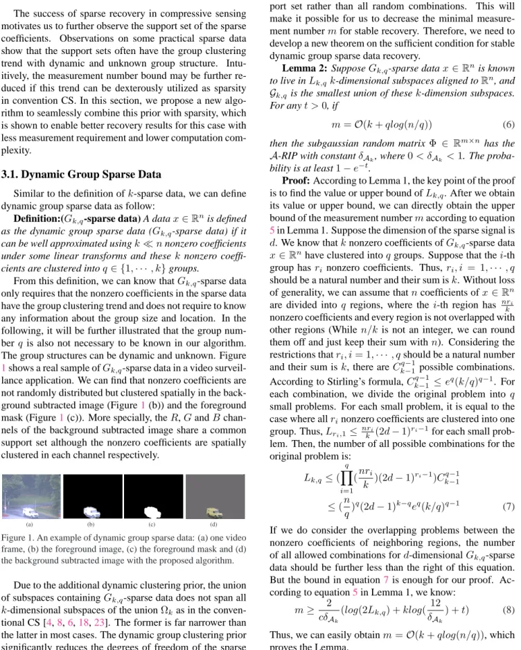
surveil-lance application. We can find that nonzero coefficients are not randomly distributed but clustered spatially in the back-ground subtracted image (Figure1(b)) and the foreground mask (Figure1(c)). More specially, theR,GandB chan-nels of the background subtracted image share a common support set although the nonzero coefficients are spatially clustered in each channel respectively.
(a) (b) (c) (d)
Figure 1. An example of dynamic group sparse data: (a) one video frame, (b) the foreground image, (c) the foreground mask and (d) the background subtracted image with the proposed algorithm.
Due to the additional dynamic clustering prior, the union of subspaces containingGk,q-sparse data does not span all
k-dimensional subspaces of the unionΩkas in the
conven-tional CS [4,8,6,18,23]. The former is far narrower than the latter in most cases. The dynamic group clustering prior significantly reduces the degrees of freedom of the sparse
signal since it only permits certain combinations of its sup-port set rather than all random combinations. This will make it possible for us to decrease the minimal measure-ment numbermfor stable recovery. Therefore, we need to develop a new theorem on the sufficient condition for stable dynamic group sparse data recovery.
Lemma 2: SupposeGk,q-sparse datax∈Rn is known
to live inLk,qk-dimensional subspaces aligned toRn, and
Gk,qis the smallest union of thesek-dimension subspaces.
For anyt >0, if
m=O(k+qlog(n/q)) (6)
then the subgaussian random matrix Φ ∈ Rm×n has the
A-RIP with constantδAk, where0< δAk <1. The
proba-bility is at least1−e−t.
Proof: According to Lemma 1, the key point of the proof
is to find the value or upper bound ofLk,q. After we obtain
its value or upper bound, we can directly obtain the upper bound of the measurement numbermaccording to equation 5in Lemma 1. Suppose the dimension of the sparse signal is d. We know thatknonzero coefficients ofGk,q-sparse data
x∈Rnhave clustered intoqgroups. Suppose that thei-th
group hasri nonzero coefficients. Thus, ri, i = 1,· · · , q
should be a natural number and their sum isk. Without loss of generality, we can assume thatncoefficients ofx∈Rn are divided into qregions, where the i-th region has nri
k
nonzero coefficients and every region is not overlapped with other regions (Whilen/k is not an integer, we can round them off and just keep their sum withn). Considering the restrictions thatri, i= 1,· · ·, qshould be a natural number
and their sum isk, there areCkq−−11 possible combinations. According to Stirling’s formula,Ckq−−11 ≤eq(k/q)q−1. For each combination, we divide the original problem into q small problems. For each small problem, it is equal to the case where allrinonzero coefficients are clustered into one
group. Thus,Lri,1≤
nri
k (2d−1)ri−1for each small
prob-lem. Then, the number of all possible combinations for the original problem is:
Lk,q≤( q Y i=1 (nri k )(2d−1) ri−1)Cq−1 k−1 ≤(n q) q(2d−1)k−qeq(k/q)q−1 (7)
If we do consider the overlapping problems between the nonzero coefficients of neighboring regions, the number of all allowed combinations ford-dimensionalGk,q-sparse
data should be further less than the right of this equation. But the bound in equation7is enough for our proof. Ac-cording to equation5in Lemma 1, we know:
m≥ 2
cδAk
(log(2Lk,q) +klog(12
δAk
) +t) (8)
Thus, we can easily obtainm=O(k+qlog(n/q)), which proves the Lemma.
Lemma 2 shows that the number of measurements re-quired for robustly recovering dynamic group sparsity data ism=O(k+qlog(n/q)), which is a significant improve-ment over the m = O(k+klog(n/k))that would be re-quired by conventional CS recovery algorithms [4,8,18, 23]. While the group numberqis smaller, more improve-ments can be obtained. Whileqis far smaller thankandk is close tolog(n), we can getm=O(k). Note that, this is a sufficient condition. If we know more priors about group settings, we can further reduce this bound.
3.2. Dynamic Group Sparsity Recovery
Lemma 2 equips us to propose a new recovery algorithm for dynamic group sparse data, namely dynamic group spar-sity (DGS) recovery algorithm. From the introduction, we know that only the SP [6] and the CoSaMP [18] have better balance between theoretical guarantee and compu-tation complexity among existing greedy recovery algo-rithms. Actually, these two algorithms have a similar frame-work. In this section, we demonstrate how to seamlessly in-tegrate the dynamic group clustering prior into that frame-work.
Our algorithm includes five main steps in each iteration: 1) pruning the residue estimation; 2) merging the support sets; 3) estimating the signal by least square; 4) pruning the signal estimation and 5) updating the signal/residue estima-tion and support set. One can observe that it is similar to that of SP/CoSaMP algorithms. The difference only exists in the pruning process in step 1 and step 4. The modification is simple. We prune the estimation in the step 1 and step 4 using DGS approximation pruning rather thank-sparse ap-proximation, as we only need to search over subspaces of
Ak,q instead of Cnk subspaces of Ωk. It directly leads to
fewer measurement requirement for stable data recovery. The DGS pruning algorithm is described in algorithm1. There exist two prior-dependent parametersJyandJb. Jy
is the number of tasks if the problem can be represented as a multi-task CS problem [13].Jbis the block size if the
inter-ested problem can be modelled as a block sparsity problem [1,24,22,26]. Their default values are set as1, which is the case of traditional sparse recovery in compressive sens-ing. Moreover, there are two important user-tuning parame-ters, the weight w of neighbors and the neighbor number τ of each element in sparse data. In practice, it is very straightforward to adjust them since they have the physi-cal meanings. The first one controls the balance between the sparsity prior and the group clustering prior. Whilewis smaller/bigger, it means that the degree of dynamic group clustering is lower/higher in the sparse signal. Generally, they are set as0.50sif there are not more knowledge about
that in practice. The parameter τ controls the number of neighbors that can be affected by each element in sparse data. Generally, it is good enough to set it as 2, 4 and 6 for
Algorithm 1. DGS approximation pruning
Input: x∈ Rn{estimations};k{the sparsity number};
Jy{task number};Jb{block size};Nx∈Rn×τ{values
of x’s neighbors};w∈Rn×τ{weights for neighbors};τ
{neighbor number} Jx=JyJb;x∈Rnis shaped tox∈R n Jx×Jx Nx∈Rn×τis shape toNx∈R n Jx×Jx×τ; for alli= 1, ...,Jn x do
Combing each entry with its neighbors
z(i) = Jx X j=1 x2(i, j) + Jx X j=1 τ X t=1 w2(i, t)Nx2(i, j, t) end for
Ω∈RJxn×1is set as indices corresponding to the largest
k/Jxentries ofz
for allj= 1, ..., Jxdo
for alli= 1, ..., k Jx do
Obtain the final list
Γ((j−1) k Jx +i) = (j−1) k Jx + Ω(i) end for end for Output:supp(x, k)←Γ
1D, 2D and 3D data respectively.
Up to now, we assume that we know the sparsity number kof the sparse data before recovery. However, it is not al-ways true in practical applications. For example, we do not know the exact sparsity numbers of the background sub-tracted images although we know they tend to be dynamic group sparse. Motivated by the idea in [7], we develop a new recovery algorithm called AdaDGS by incorporating an adaptive sparsity scheme into the above DGS recovery algorithm.
Suppose the range of the sparsity number is known to be[kmin, kmax]. We can set the step size of sparsity
num-ber as 4k. The whole recovery process is divided into several stages, each of which includes several iterations. Thus, there are two loops in AdaDGS recovery algorithm. The sparsity number is initialized as kmin before
itera-tions. During each stage (inner loop), we iteratively opti-mize sparse data with the fixed sparsity numberkcurruntil
the halting condition within the stage is true (for example, the residue norm is not decreasing). We then switch to the next stage after adding4kinto the current sparsity number kcurr (outer loop). The whole iterative process will stop
whenever the halting condition is satisfied. For practical applications, there is a trade-off between the sparsity step size4kand the recovery performance. Smaller step sizes require more iterations and bigger step size may cause
in-Algorithm 2. AdaDGS Recovery
1: Input: Φ∈ Rm×n{sample matrix};y ∈ Rm{sample
vector};[kmin, kmax] {sparsity range}; 4k {sparsity
step size}
2: Initialization: residue yr = y; Γ = supp(x) = ∅;
sparse datax= 0; sparsity numberk=kmin
3: repeat
4: Perform DGS recovery algorithm with sparsity num-berkto obtainxand the residue
5: if halting criterion false then
6: UpdateΓ,yrandk=k+4k
7: end if
8: until halting criterion true
9: Output:x= Φ†Γy
accuracy. The sparsity range depends on the applications. Generally, it can be set as[1, n/3], wherenis the dimen-sion of the sparse data. Algorithm2describes the proposed AdaDGS recovery algorithm.
3.3. AdaDGS Background Subtraction
Background subtraction is an important pre-processing step in video monitoring applications. There exist a lot of methods for this problem. The Mixture of Gaussians (MoG) background model assumes the color evolution of each pixel can be modelled as a MoG and are widely used on realistic scenes [21]. Elgammal et al. [10] proposed a non-parametric model for the background under similar computational constraints as the MoG. Spatial constraints are also incorporated into their model. Sheikh and Shah consider both temporal and spatial constraints in a Bayesian framework [20], which results in good foreground segmen-tations even when the background is dynamic. The model in [16] also uses a similar scheme. All these methods only im-plicitly model the background dynamics. In order to better handle dynamic scenes, some recent works [17,27] explic-itly model the background as dynamic textures. Most dy-namic texture modeling methods are based on the Auto Re-gressive and Moving Average (ARMA) model, whose dy-namics is driven by a linear dynamic system (LDS). While this linear model can handle background dynamics with cer-tain stationarity, it will cause over-fitting for more complex scenes.
The inspiration for our AdaDGS background subtraction came from the success in online DT video registration based on the sparse representation constancy assumption (SRCA) [12]. The SRCA states that a new coming video frame should be represented as a linear combination of as few preceding image frames as possible. As a matter of fact, the traditional brightness constancy assumption seeks that the current video frame can be best represented by a
sin-gle preceding frame, while the SRCA seeks that the current frame can be best sparsely represented by all preceding im-age frames. Thus, the former can be thought as a special case of SRCA.
Suppose a video sequence consists of framesI1, ..., In ∈
Rm. Without loss of generality, we can assume that
back-ground subtraction has already been performed on the first tframes. LetA = [I1, ..., It] ∈ Rm×t. Denote the
back-ground image and the backback-ground subtracted image by b andf, respectively, forIt+1. From the introduction in Sec-tion3.1, we know thatfis dynamic group sparse data with unknown sparsity numberkfand group structure.
Accord-ing to SRCA, we haveb=Ax, wherex∈Rtshould bek x
-sparse vector andkx << t. LetΦ = [A, I] ∈Rm×(t+m),
whereI∈Rm×mis an identity matrix. Then, we have:
It+1=Ax+f = [A, I] · x f ¸ = Φz (9)
wherez ∈ Rt+mis the DGS data with unknown sparsity
kx+kf. Background subtraction is thus formulated as the
following AdaDGS recovery problem:
(x0, f0) =argminkzk0, kIt+1−Φzk2< ε (10) which can be efficiently solved by the proposed AdaDGS recovery algorithm. Similar ideas are used for face recogni-tion robust to occlusion [25]. It is worth menrecogni-tioning that the coefficients inwcorresponding to thexpart are randomly sparse while those corresponding to f are dynamic group sparse. During the DGS approximation pruning, we thus can set those coefficients in weightwfor thex-related part as zeros and those forf as nonzeros. Since we do not know the sparsity numberkxandkf, we can set sparsity ranges
for them respectively and run the AdaDGS recovery algo-rithm until the halting condition is true. Then, we can obtain the optimized background subtracted image f and back-ground imageb=Ax. For long video sequences, it is im-practical to build a model matrixA = [I1, ..., It]∈Rm×t,
wheret denotes the last frame number. In order to cope with this case, we can set a time window width parameter τ. We then build the model matrix,A= [It−τ+1, ..., It]∈
Rm×(t−τ), for the(t+ 1)frame, which can avoid the mem-ory requirement blast for a long video sequence. The com-plete algorithm for AdaDGS based background subtraction is summarized in Algorithm3.
4. Experiments
For quantitative evaluation, the recovery error is defined to indicate the difference between the estimationxestand
the ground-truthx:kxest−xk2/kxk2. All experiments are conducted on a3.2GHzPC in Matlab environment.
Algorithm 3. AdaDGS Background Subtraction 1: Input: The video sequence I1, ..., In, the number t
which means 1st ∼ tth have been performed
back-ground subtraction, the time window widthτ≤t
2: for allj=t+ 1, ..., ndo
3: SetA= [Ij−τ, ..., Ij−1]and formΦ = [A, I]
4: Sety=Ijand the sparsity ranges/step-sizes
5: (x0, f0) =AdaDGS(Φ, y)
6: end for
7: Output: Background subtracted images
4.1. 1D Simulated Signals
In the first experiment, we randomly generate a 1D G(k, q)-sparse signal with values ±1, where n = 512, k = 64andq = 4. The projection matrixΦis generated by creating am×nmatrix with i.i.d. draws of a Gaussian distribution N(0; 1), and then the rows of Φare normal-ized to the unit magnitude. Zero-mean Gaussian noise with standard deviationσ= 0.01is added to the measurements. Figure2 shows one generated signal and its recovered re-sults by different algorithms when m = 3k = 192. As the measurement numbermis only3times of the sparsity numberk, both of other algorithms can not obtain good covery results, whereas the DGS obtains almost perfect re-covery results with the least running time. To study how the measurement number m effects the recovery perfor-mance, we change the measurement number and record the recovery results by different algorithms. To reduce the ran-domness, we execute the experiment 100 times for each of the measurement numbers in testing each algorithm. Fig-ure3shows the performance of 5 algorithms with increas-ing measurements in terms of the recovery error and run-ning time. Overall, the DGS obtains the best recovery per-formance with the least computation; the recovery perfor-mance of GPSR, SPGL1-Lasso and SP is close; and the l1−norm minimization based GPSR and SPGL1-Lasso re-quire more computation than greedy algorithms such as the OMP, SP and our DGS. In the three greedy algorithms, the OMP has the worst recovery performance. All these ex-perimental results are consistent with our theorem: the pro-posed DGS algorithm can achieve better recovery perfor-mance for DGS data with far few measurements and less computation complexity.
4.2. 2D Color Images
To validate the proposed recovery algorithm on 2D im-ages, we randomly generate a 2D G(k, q)-sparse color image by putting four digits in random locations, where
n = H ∗W = 48∗48,k = 152andq = 4. The
pro-jection matrixΦand noises are generated with the similar method as that for 1D signal. TheG(k, q)-sparse color
im-100 200 300 400 500 -1
0 1
(a) Original Signal
100 200 300 400 500 -1 0 1 (b) GPSR 100 200 300 400 500 -1 0 1 (c) SPGL1-LASSO 100 200 300 400 500 -1 0 1 (d) OMP 100 200 300 400 500 -1 0 1 (e) SP 100 200 300 400 500 -1 0 1 (f) DGS
Figure 2. Recovery results of 1D data. (a) Original data; (b) GPSR (error is 0.5173 and time is 0.1847 seconds); (c) SPGL1-Lasso (error is 0.4021 and time is 1.1497 seconds); (d) OMP (error is 1.0270 and time is 0.1422 seconds);(e) SP (error is 0.6143 and time is 0.1100 seconds);(f) DGS recovery (error is 0.0178 and time is 0.0605 seconds). 160 170 180 190 200210 220 230 240 250 260 -0.2 0 0.2 0.4 0.6 0.8 1 1.2 1.4 1.6 R e c o v e ry E rr o r Measurement Number GPSR SPGL1-LASSO OMP SP DGS (a) 160 170 180 190 200 210 220 230 240 250 260 0 0.5 1 1.5 2 2.5 R u n n in g T im e ( S e c o n d ) Mesurement Number GPSR SPGL1-LASSO OMP SP DGS (b)
Figure 3. Recovery errors vs. measurement numbers: a) recovery errors; (b) running times
age has a special property: the R, G and B channels share a common support set, while the nonzero coefficients have dynamic group clustering trends within each channel. Thus, the recovery of DGS color images can be considered as a
3-task CS recovery problem. As for the input parameters of DGS in this case, we just need to setJy as 3and keep
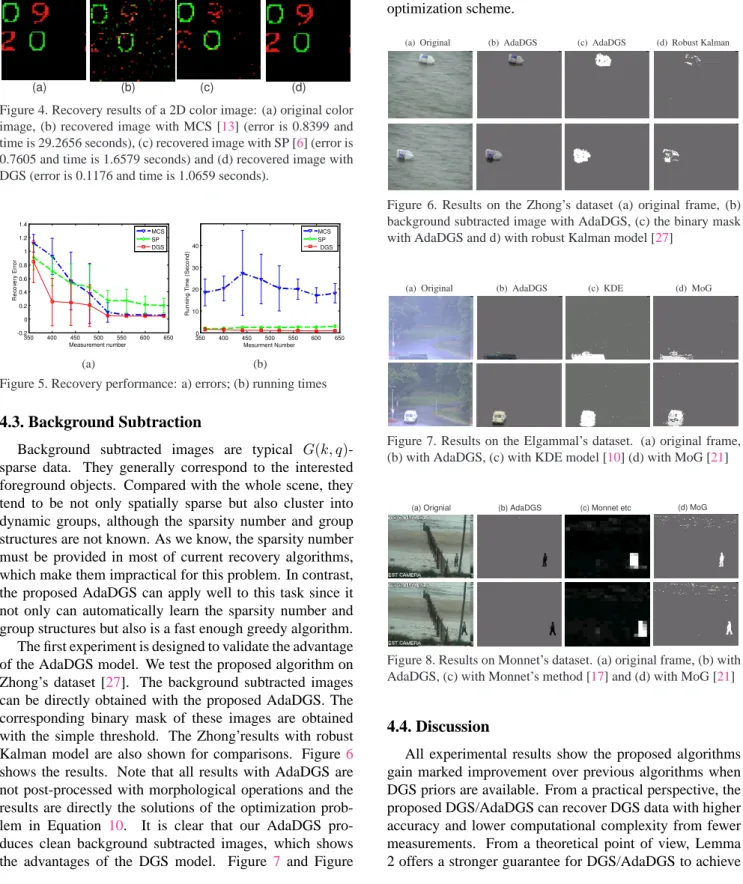
other default parameters unchanged. Considering the MCS is specially designed for multi-task CS problems, we will compare it with DGS and SP. Figure4shows one example 2DG(k, q)-sparse color image and the recovered results by different algorithms whenm = 440. Figure5 shows the performance of the three algorithm, averaged over 100 ran-dom runs for each sample size. The DGS achieves the best recovery performance with far less computation. It is easily understood because DGS exploits three priors for recovery: (1) the three color channels share a common support set, (2) there are dynamic group clustering trends within each color channel and (3) sparsity prior exists in each channel; thus it achieves better results than MCS, which only uses two priors. The SP is the worst since it only uses one prior. This experiment clearly demonstrates: the more valid priors are used for sparse recovery, the more accurate results we can achieve. That is the main reason why DGS, MCS and SP obtained the best, good and the worst recovery results.
Figure5(b) shows the comparison of running times by the three algorithms. It is not surprising that the running times with DGS are always far less than those with MCS and a little less than those with SP for all measurement numbers.
(a) (b) (c) (d) Figure 4. Recovery results of a 2D color image: (a) original color image, (b) recovered image with MCS [13] (error is 0.8399 and time is 29.2656 seconds), (c) recovered image with SP [6] (error is 0.7605 and time is 1.6579 seconds) and (d) recovered image with DGS (error is 0.1176 and time is 1.0659 seconds).
350 400 450 500 550 600 650 -0.2 0 0.2 0.4 0.6 0.8 1 1.2 1.4 R e c o ve ry E rr o r Measurement number MCS SP DGS (a) 3500 400 450 500 550 600 650 10 20 30 40 R u n n in g T im e ( S e c o n d ) Mesurment Number MCS SP DGS (b)
Figure 5. Recovery performance: a) errors; (b) running times
4.3. Background Subtraction
Background subtracted images are typical G(k, q) -sparse data. They generally correspond to the interested foreground objects. Compared with the whole scene, they tend to be not only spatially sparse but also cluster into dynamic groups, although the sparsity number and group structures are not known. As we know, the sparsity number must be provided in most of current recovery algorithms, which make them impractical for this problem. In contrast, the proposed AdaDGS can apply well to this task since it not only can automatically learn the sparsity number and group structures but also is a fast enough greedy algorithm. The first experiment is designed to validate the advantage of the AdaDGS model. We test the proposed algorithm on Zhong’s dataset [27]. The background subtracted images can be directly obtained with the proposed AdaDGS. The corresponding binary mask of these images are obtained with the simple threshold. The Zhong’results with robust Kalman model are also shown for comparisons. Figure6 shows the results. Note that all results with AdaDGS are not post-processed with morphological operations and the results are directly the solutions of the optimization prob-lem in Equation 10. It is clear that our AdaDGS pro-duces clean background subtracted images, which shows the advantages of the DGS model. Figure 7 and Figure
8 show the background subtraction results on two other videos [10,17]. Note that our results without postprocess-ing can compete with others with postprocesspostprocess-ing. The re-sults show the proposed AdaDGS model can handle well highly dynamic scenes by exploiting the effective sparsity optimization scheme.
(a) Original (b) AdaDGS (c) AdaDGS (d) Robust Kalman
Figure 6. Results on the Zhong’s dataset (a) original frame, (b) background subtracted image with AdaDGS, (c) the binary mask with AdaDGS and d) with robust Kalman model [27]
(a) Original (b) AdaDGS (c) KDE (d) MoG
Figure 7. Results on the Elgammal’s dataset. (a) original frame, (b) with AdaDGS, (c) with KDE model [10] (d) with MoG [21]
(a) Orignial (b) AdaDGS (c) Monnet etc (d) MoG
Figure 8. Results on Monnet’s dataset. (a) original frame, (b) with AdaDGS, (c) with Monnet’s method [17] and (d) with MoG [21]
4.4. Discussion
All experimental results show the proposed algorithms gain marked improvement over previous algorithms when DGS priors are available. From a practical perspective, the proposed DGS/AdaDGS can recover DGS data with higher accuracy and lower computational complexity from fewer measurements. From a theoretical point of view, Lemma 2 offers a stronger guarantee for DGS/AdaDGS to achieve
stable recovery. Moreover, we provide a generalized frame-work for priors-driven sparse data recovery algorithms. Us-ing different input parameter settUs-ings, it can perform sparse recovery, multi-task sparse recovery, group/block sparse re-covery, DGS rere-covery, and adaptive DGS rere-covery, respec-tively. Group structure and sparsity number are not must-knows for our algorithm, which makes it flexible and ap-plicable in many practical applications; as far as we know, this property of our algorithm is unique among all existing sparse recovery algorithms.
5. Conclusions
In this paper, we extend the theory of CS to efficiently handle dynamic group sparse data. Based on this ex-tended theory, the proposed algorithm can stably recover dynamic group-sparse data using far fewer measurements and less computation than the current state-of-the-art al-gorithms with provable guarantees. It has been applied to sparse recovery and background subtraction on both simu-lated and practical data. Experimental results demonstrate the performance guarantee of the proposed algorithm and show marked improvement over previous algorithms.
References
[1] E. Berg, M. Schmidt, M. Friedlander, and K. Murphy. Group sparsity via linear-time projection. 2008. Preprint. 2,4 [2] T. Blumensath and M. Davies. Sampling theorems for
sig-nals from the union of finite-dimensional linear subspaces.
IEEE Transactions on Information Theory, 2008. Accepted. 2
[3] E. Candes. Compressive sampling. In Proceedings of the
International Congress of Mathematicians, 2006. 2 [4] E. Candes, J. Romberg, and T. Tao. Robust uncertainty
prin-ciples: Exact signal reconstruction from highly incomplete frequency information. IEEE Transactions on Information
Theory, 52:489–509, 2006. 1,3,4
[5] S. Chen, D. Donoho, and M. Saunders. Atomic decomposi-tion by basis pursuit. SIAM Journal on Scienticifc
Comput-ing, 61:20–33, 1998. 1
[6] W. Dai and O. Milenkovic. Subspace pursuit for compres-sive sensing: closing the gap between performance and com-plexsity, 2008. Preprint. 1,3,4,7
[7] T. Do, L. Gan, N. Nguyen, and T. Tran. Sparsity adaptive matching pursuit algorithm for practical compressed sensing. 2008. Accepted. 4
[8] D. Donoho. Compressed sensing. IEEE Transactions on
Information Theory, 52:1289–1306, 2006. 1,2,3,4 [9] D. Donoho, Y. Tsaig, I. Drori, and J. Starck. Sparse solution
of underdetermined linear equations by stagewise orthogonal matching pursuit, 2007. Submitted. 1
[10] A. Elgammal, D. Harwood, and L. Davis. Non-parametric model for background subtraction. In Proceedings of ECCV, 2000. 5,7
[11] M. Figueiredo, R. Nowak, and S. Wright. Gradient pro-jection for sparse reconstruction: application to compressed sensing and other inverse problems. IEEE Journal on
Se-lected Topics in Signal Processing, 1(4):586–597, 2007. 1 [12] J. Huang, X. Huang, and D. Metaxas. Simultaneous image
transformation and sparse representation recovery. In
Pro-ceedings of CVPR, 2008. 5
[13] S. Ji, D. Dunson, and L. Carin. Multi-task compressive sens-ing. IEEE Transactions on Signal Processing, 2008. Sub-mitted. 2,4,7
[14] S. Kim, K. Koh, M. Lustig, S. Boyd, and D. Gorinevsky. A method for large-scale l1-regularized least squares. IEEE
Journal on Selected Topics in Signal Processing, 1(4):606–
607, 2007. 1
[15] S. Mallat and Z. Zhang. Matching pursuits with time-frequency dictionaries. IEEE Transactions on Signal
Pro-cessing, 41(12):3397–3415, 1993. 1
[16] A. Mittal and M. Paragios. Motion-based background sub-traction using adaptive kernel density estimation. In
Pro-ceedings of CVPR, 2004. 5
[17] A. Monnet, A. Mittal, N. Paragios, and Y. Ramesh. Back-ground modeling and subtraction of dynamic scenes. In
Pro-ceedings of ICCV, 2003. 5,7
[18] D. Needell and J. Tropp. Cosamp: Iterative signal recovery from incomplete and inaccurate samples. Applied and
Com-putational Harmonic Analysis, 2008. Accepted. 1,3,4 [19] D. Needell and R. Vershynin. Signal recovery from
incom-plete and inaccurate measurements via regularized orthogo-nal matching pursuit, 2007. Submitted. 1
[20] Y. Sheikh and M. Shah. Bayesian modeling of dynamic scenes for object detection. In IEEE Transactions on
Pat-tern Analysis and Machine Intelligence, volume 27, 2005. 5
[21] C. Stauffer and W. Grimson. Adaptive background mixture models for real-time tracking. 2:246–252, 1999. 5,7 [22] M. Stojnic, F. Parvaresh, and B. Hassibi. On the
reconstruc-tion of block-sparse signals with an optimal number of mea-surements. 2008. Preprint. 2,4
[23] J. Tropp and A. Gilbert. Signal recovery from random mea-surements via orthogonal matching pursuit. IEEE
Transac-tions on Information Theory, 53(12):4655–4666, 2007. 1,3,
4
[24] J. Tropp, A. Gilbert, and M. Strauss. Algorithms for simul-taneous sparse approximation. part i: Greedy pursuit. IEEE
Transactions on Signal Processing, 86:572–588, 2006. 2,4 [25] J. Wright, A. Yang, A. Ganesh, S. Sastry, and Y. Ma. Robust face recognition via sparse representation. IEEE Transactions on Pattern Analysis and Machine Intelligence,
31(2):210–227, 2009. 5
[26] M. Yuan and Y. Lin. Model selection and estimation in re-gression with grouped variables. Journal of The Royal
Sta-tistical Society Series B, 68(1):49–67, 2006. 2,4
[27] J. Zhong and S. Sclaroff. Segmenting foreground objects from a dynamic textured background via a robust kalman fil-ter. In Proceedings of ICCV, 2003. 5,7