Multi-Sampled Imaging with Structural Models
Shree K. Nayar and Srinivasa G. Narasimhan Department of Computer Science, Columbia University
New York, NY 10027, U.S.A. {nayar, srinivas}cs.columbia.edu
Abstract. Multi-sampled imaging is a general framework for using pix-els on an image detector to simultaneously sample multiple dimensions of imaging (space, time, spectrum, brightness, polarization, etc.). The mosaic of red, green and blue spectral filters found in most solid-state color cameras is one example of multi-sampled imaging. We briefly de-scribe how multi-sampling can be used to explore other dimensions of imaging. Once such an image is captured, smooth reconstructions along the individual dimensions can be obtained using standard interpolation algorithms. Typically, this results in a substantial reduction of resolution (and hence image quality). One can extract significantly greater resolu-tion in each dimension by noting that the light fields associated with real scenes have enormous redundancies within them, causing different dimensions to be highly correlated. Hence, multi-sampled images can be better interpolated using local structural models that are learned off-line from a diverse set of training images. The specific type of structural models we use are based on polynomial functions of measured image in-tensities. They are very effective as well as computationally efficient. We demonstrate the benefits of structural interpolation using three specific applications. These are (a) traditional color imaging with a mosaic of color filters, (b) high dynamic range monochrome imaging using a mo-saic of exposure filters, and (c) high dynamic range color imaging using a mosaic of overlapping color and exposure filters.
1
Multi-Sampled Imaging
Currently, vision algorithms rely on images with 8 bits of brightness or color at each pixel. Images of such quality are simply inadequate for many real-world applications. Significant advances in imaging can be made by exploring the fun-damental trade-offs that exist between various dimensions of imaging (see Figure 1). The relative importances of these dimensions clearly depend on the applica-tion at hand. In any practical scenario, however, we are given a finite number of pixels (residing on one or more detectors) to sample the imaging dimensions. Therefore, it is beneficial to view imaging as the judicious assignment of resources (pixels) to the dimensions of imaging that are relevant to the application.
Different pixel assignments can be viewed as different types of samplings of the imaging dimensions. In all cases, however, more than one dimension is simul-taneously sampled. In the simplest case of a gray-scale image, image brightness and image space are sampled, simultaneously. More interesting examples result from using image detectors made of an assortment of pixels, as shown in Figure
brightness spectrum depth space time polarization
Fig. 1.A few dimensions of imaging. Pixels on an image detector may be assigned to multiple dimensions in a variety of ways depending on the needs of the application.
2. Figure 2(a) shows the popular Bayer mosaic [Bay76] of red, green and blue spectral filters placed adjacent to pixels on a detector. Since multiple color mea-surements cannot be captured simultaneously at a pixel, the pixels are assigned to specific colors to trade-off spatial resolution for spectral resolution. Over the last three decades various color mosaics have been suggested, each one resulting in a different trade-off (see [Dil77], [Dil78], [MOS83], [Par85], [KM85]).
Historically, multi-sampled imaging has only been used in the form of color mosaics. Only recently has the approach been used to explore other imaging dimensions. Figure 2(b) shows the mosaic of neutral density filters with different transmittances used in [NM00] to enhance an image detector’s dynamic range. In this case, spatial resolution is traded-off for brightness resolution (dynamic range). In [SN01], spatially varying transmittance and spectral filters were used with regular wide FOV mosaicing to yield high dynamic range and multi-spectral mosaics. Figure 2(c) shows how space, dynamic range and color can be sampled simultaneously by using a mosaic of filters with different spectral responses and transmittances. This type of multi-sampling is novel and, as we shall show, results in high dynamic range color images. Another example of assorted pixels was proposed in [BE00], where a mosaic of polarization filters with different orientations is used to estimate the polarization parameters of light reflected by scene points. This idea can be used in conjunction with a spectral mosaic, as shown in Figure 2(d), to achieve simultaneous capture of polarization and color. Multi-sampled imaging can be exploited in many other ways. Figures 2(e) shows how temporal sampling can be used with exposure sampling. This ex-ample is related to the idea of sequential exposure change proposed in [MP95], [DM97] and [MN99] to enhance dynamic range. However, it is different in that the exposure is varied as a periodic function of time, enabling the generation of high dynamic range, high framerate video. The closest implementation appears to be the one described in [GHZ92] where the electronic gain of the camera is varied periodically to achieve the same effect. A more sophisticated implementa-tion may sample space, time, exposure and spectrum, simultaneously, as shown in Figure 2(f).
The above examples illustrate that multi-sampling provides a general frame-work for designing imaging systems that extract information that is most
per-R G R G R G R G R G R G R G R G R G R G R G R G R G R G R G R G R G R G R G R G R G R G R G R G R G R G R G R G R G R G R G R G R G R G R G R G G B G B G B G B G B G B G B G B G B G B G B G B G B G B G B G B G B G B G B G B G B G B G B G B G B G B G B G B G B G B G B G B G B G B G B G B R R R R R R R R R B B B B B B B B B G G G G G G G G G G G G G G G G G G R R R R R R R R R B B B B B B B B B G G G G G G G G G G G G G G G G G G R R R R R R R R R B B B B B B B B B G G G G G G G G G G G G G G G G G G R R R R R R R R R B B B B B B B B B G G G G G G G G G G G G G G G G G G R G R G R G R G R G R G R G R G R G R G R G R G R G R G R G R G R G R G R G R G R G R G R G R G R G R G R G R G R G R G R G R G R G R G R G R G G B G B G B G B G B G B G B G B G B G B G B G B G B G B G B G B G B G B G B G B G B G B G B G B G B G B G B G B G B G B G B G B G B G B G B G B R G R G R G R G R G R G R G R G R G R G R G R G R G R G R G R G R G R G R G R G R G R G R G R G R G R G R G R G R G R G G R G R G R G R G R G G B G B G B G B G B G B G B G B G B G B G B G B G B G B G B G B G B G B G B G B G B G B G B G B G B G B G B G B G B G B G B G B G B G B G B G B R G R G R G R G R G R G R G R G R R G R G R R G R R G R R G G R G R G R G R R G R R G R G R G R G R R G R R G R G G B G B G B G B G B G B G B G B G B G B G B G B G B G B G B G B G B G B G B G B G B G B G B G B G G B G B G B G B G B G B G B G B G B G B G B R G R G R G R G R G R G R G R G R G R G R G R G R G R G R G R G R G R G R G R G R G R G R G R G R G R G R G R G R G R G R G R G R G R G R G R G G B G B G B G B G B G B G B G B G B G B G B G B G B G B G G B G B G B G B G B G B G B G B G B G B G B G B G B G B G B G B G B G B G B G B G B B time time (a) (b) (c) (d) (e) (f)
Fig. 2. A few examples of multi-sampled imaging using assorted pixels. (a) A color mosaic. Such mosaics are widely used in solid-state color cameras. (b) An exposure mosaic. (c) A mosaic that includes different colors and exposures. (d) A mosaic using color and polarization filters. (e), (f) Multi-sampling can also involve varying exposure and/or color over space and time.
tinent to the application. Though our focus is on the visible light spectrum, multi-sampling is, in principle, applicable to any form of electromagnetic radia-tion. Therefore, the pixel assortments and reconstruction methods we describe in this paper are also relevant to other imaging modalities such as X-ray, magnetic resonance (MR) and infra-red (IR). Furthermore, the examples we discuss are two-dimensional but the methods we propose are directly applicable to higher-dimensional imaging problems such as ones found in tomography and microscopy.
2
Learned Structural Models for Reconstruction
How do we reconstruct the desired image from a captured multi-sampled one? Nyquist’s theory [Bra65] tells us that for a continuous signal to be perfectly re-constructed from its discrete samples, the sampling frequency must be at least twice the largest frequency in the signal. In the case of an image of a scene, the optical image is sampled at a frequency determined by the size of the de-tector and the number of pixels on it. In general, there is no guarantee that this sampling frequency satisfies Nyquist’s criterion. Therefore, when a tradi-tional interpolation technique is used to enhance spatial resolution, it is bound to introduce errors in the form of blurring and/or aliasing. In the case of multi-sampled images (see Figure 2), the assignment of pixels to multiple dimensions causes further undersampling of scene radiance along at least some dimensions. As a result, conventional interpolation methods are even less effective.
Our objective is to overcome the limits imposed by Nyquist’s theory by using prior models that capture redundancies inherent in images. The physical struc-tures of real-world objects, their reflectances and illuminations impose strong constraints on the light fields of scenes. This causes different imaging dimen-sions to be highly correlated with each other. Therefore, a local mapping func-tion can be learned from a set of multi-sampled images and their corresponding correct (high quality) images. As we shall see, it is often beneficial to use multi-ple mapping functions. Then, given a novel multi-sammulti-pled image, these mapping functions can be used to reconstruct an image that has enhanced resolution in each of the dimensions of interest. We refer to these learned mapping functions as local structural models.
The general idea of learning interpolation functions is not new. In [FP99], a probabilistic Markov network is trained to learn the relationship between sharp and blurred images, and then used to increase spatial resolution of an image. In [BK00], a linear system of equations is solved to estimate a high resolution image from a sequence of low resolution images wherein the object of interest is in motion. Note that both these algorithms are developed to improvespatial
resolution, while our interest is in resolution enhancement along multiple imaging dimensions.
Learning based algorithms have also been applied to the problem of interpo-lating images captured using color mosaics. The most relevant among these is the work of Wober and Soini [WS95] that estimates an interpolation kernel from training data (high quality color images of test patterns and their correspond-ing color mosaic images). The same problem was addressed in [Bra94] uscorrespond-ing a Bayesian method.
We are interested in a general method that can interpolate not just color mosaic images but any type of multi-sampled data. For this, we propose the use of a structural model where each reconstructed value is a polynomial function of the image brightnesses measured within a local neighborhood. The size of the neighborhood and the degree of the polynomial vary with the type of multi-sampled data being processed. It turns out that the model of Wober and Soini [WS95] is a special instance of our model as it is a first-order polynomial applied to the specific case of color mosaic images. As we shall see, our polynomial model produces excellent results for a variety of multi-sampled images. Since it uses polynomials, our method is very efficient and can be easily implemented in hardware. In short, it is simple enough to be incorporated into any imaging device (digital still or video camera, for instance).
3
Training Using High Quality Images
Since we wish to learn our model parameters, we need a set of high quality training images. These could be real images of scenes, synthetic images generated by rendering, or some combination of the two. Real images can be acquired using professional grade cameras whose performance we wish to emulate using lower quality multi-sampling systems. Since we want our model to be general, the set of training images must adequately represent a wide range of scene features. For instance, images of urban settings, landscapes and indoor spaces may be included. Rotated and magnified versions of the images can be used to capture the effects of scale and orientation. In addition, the images may span the gamut of illumination conditions encountered in practice, varying from indoor lighting to overcast and sunny conditions outdoor. Synthetic images are useful as one can easily include in them specific features that are relevant to the application.
Fig. 3. Some of the 50 high quality images (2000 x 2000 pixels, 12 bits per color channel) used to train the local structural models described in Sections 4, 5 and 6.
Some of the 50 high quality images we have used in our experiments are shown in Figure 3. Each of these is a 2000 x 2000 color (red, green, blue) image with 12 bits of information in each color channel. These images were captured using a film camera and scanned using a 12-bit slide scanner. Though the total
number of training images is small they include a sufficiently large number of local (say, 7×7 pixels) appearances for training our structural models.
Given such high quality images, it is easy to generate a corresponding set of low-quality multi-sampled images. For instance, given a 2000×2000 RGB image with 12-bits per pixel, per color channel, simple downsampling in space, color, and brightness results in a 1000×1000, 8 bits per pixel multi-sampled image with the sampling pattern shown in Figure 2(c). We refer to this process of generating multi-sampled images from high quality images asdowngrading.
With the high quality images and their corresponding (downgraded) multi-sampled images in place, we can learn the parameters of our structural model. A structural model is a function f that relates measured data M(x, y) in a multi-sampled image to a desired valueH(i, j) in the high quality training image:
H(i, j) = f(M(1,1), ....,M(x, y), ....M(X, Y)) (1)
where, X and Y define some neighborhood of measured data around, or close to, the high quality valueH(i, j). Since our structural model is a polynomial, it is linear in its coefficients. Therefore, the coefficients can be efficiently computed from training data using linear regression.
Note that a single structural model may be inadequate. If we set aside the measured data and focus on the type of multi-sampling used (see Figure 2), we see that pixels can have different types of neighborhood sampling patterns. If we want our models to be compact (small number of coefficients) and effective we cannot expect them to capture variations in scenes as well as changes in the sampling pattern. Hence, we use a single structural model for each type of local sampling pattern. Since our imaging dimensions are sampled in a uniform man-ner, in all cases we have a small number of local sampling patterns. Therefore, only a small number of structural models are needed. During reconstruction, given a pixel of interest, the appropriate structural model is invoked based on the pixel’s known neighborhood sampling pattern.
4
Spatially Varying Color (SVC)
Most color cameras have a single image detector with a mosaic of red, green and blue spectral filters on it. The resulting image is hence a widely used type of multi-sampled image. We refer to it as a spatially varying color (SVC) image. When one uses an NTSC color camera, the output of the camera is nothing but an interpolated SVC image. Color cameras are notorious for producing inade-quate spatial resolution and this is exactly the problem we seek to overcome using structural models. Since this is our first example, we will use it to describe some of the general aspects of our approach.
4.1 Bayer Color Mosaic
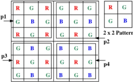
Several types of color mosaics have been implemented in the past [Bay76], [Dil77], [Dil78], [MOS83], [Par85], [KM85]. However, the most popular of these is the Bayer pattern [Bay76] shown in Figure 4. Since the human eye is more sensitive to the green channel, the Bayer pattern uses more green filters than it does red
and blue ones. Specifically, the spatial resolutions of green, red and blue are 50%, 25% and 25%, respectively. Note that the entire mosaic is obtained by repeating the 2×2 pattern shown on the right in Figure 4. Therefore, given a neighborhood size, all neighborhoods in a Bayer mosaic must have one of four possible sampling patterns. If the neighborhood is of size 3×3, the resulting patterns arep1,p2,p3andp4shown in Figure 4.
R R R R R R R R R B B B B B B B B B G G G G G G G G G G G G G G G G G G p2 p4 p1 p3 R B G G 2 x 2 Pattern
Fig. 4.Spatially varying color (SVC) pattern on a Bayer mosaic. Given a neighborhood size, all possible sampling patterns in the mosaic must be one of four types. In the case of a 3×3 neighborhood, these patterns arep1,p2,p3andp4.
4.2 SVC Structural Model
From the measured SVC image, we wish to compute three color values (red, green and blue) at each pixel, even though each pixel in the SVC image provides a single color measurement. Let the measured SVC image be denoted by M
and the desired high quality color image byH. A structural model relates each color value inHto the measured data within a small neighborhood inM. This neighborhood includes measurements of different colors and hence the model implicitly accounts for correlations between different color channels.
As shown in Figure 5, letMpbe the measured data in a neighborhood with sampling patternp, andHp(i+ 0.5, j+ 0.5, λ) be the high quality color value at the center of the neighborhood. (The center is off-grid because the neighborhood is an even number of pixels in width and height.) Then, a polynomial structural model can be written as:
Hp(i+ 0.5, j+ 0.5, λ) = (x,y)∈Sp(i,j) (k=x,l=y)∈Sp(i,j) Np n=0 Np−n q=0 Cp(a, b, c, d, λ, n)Mpn(x, y)Mpq(k, l). (2)
Sp(i, j) is the neighborhood of pixel (i, j), Np is the order of the polynomial andCpare the polynomial coefficients for the patternp. The coefficient indices
(a, b, c, d) are equal to (x−i, y−j, k−i, l−j).
The product Mp(x, y)Mp(k, l) explicitly represents the correlation between different pixels in the neighborhood. For efficiency, we have not used these cross-terms in our implementations. We found that very good results are obtained
R G B R R R B B B G G G G G G G B R G Mapping Function C M ( x, y )p H ( i+0.5, j+0.5, p λ ) ( i+0.5, j+0.5 ) S ( i, j )p Neighborhood Reconstructed Values
Fig. 5. The measured data Mp in the neighborhood Sp(i, j) around pixel (i, j) are related to the high quality color values Hp(i+ 0.5, j+ 0.5, λ) via a polynomial with coefficientsCp. A H (pλ) p p p M C (λ) ( with powers upto N )p
Fig. 6.The mapping function in (3) can be expressed as a linear system using matrices and vectors. For a given patternpand colorλ,Apis the measurement matrix,Cp(λ) is the coefficient vector andHp(λ) is the reconstruction vector.
even when each desired value is expressed as just a sum of polynomial functions of the individual pixel measurements:
Hp(i+ 0.5, j+ 0.5, λ) = (x,y)∈Sp(i,j) Np n=0 Cp(a, b, λ, n)Mpn(x, y). (3)
The mapping function (3), for each colorλ and each local pattern typep, can be conveniently rewritten using matrices and vectors, as shown in Figure 6:
Hp(λ) =ApCp(λ). (4)
For a given pattern type p and color λ, Ap is the measurement matrix. The rows ofApcorrespond to the different neighborhoods in the image that have the patternp. Each row includes all the relevant powers (up toNp) of the measured data Mp within the neighborhood. The vectorCp(λ) includes the coefficients of the polynomial mapping function and the vectorHp(λ) includes the desired high quality values at the off-grid neighborhood centers. The estimation of the model parametersCp can then be posed as a least squares problem:
Cp(λ) = (ATpAp)−1ATpHp(λ), (5) When the signal-to-noise characteristics of the image detector are known, (5) can be rewritten using weighted least squares to achieve greater accuracy [Aut01].
4.3 Total Number of Coefficients
The number of coefficients in the model (3) can be calculated as follows. Let the neighborhood size beu×v, and the polynomial order corresponding to each patternpbeNp. Let the number of distinct local patterns in the SVC image be
P and the number of color channels beΛ. Then, the total number of coefficients needed for structural interpolation is:
|C|= P+u∗v∗ P p=1 Np ∗Λ . (6)
For the Bayer mosaic, P = 4 and Λ = 3 (R,G,B). If we use Np = 2 and
u =v = 6, the total number of coefficients is 876. Since these coefficients are learned from real data, they yield greater precision during interpolation than standard interpolation kernels. In addition, they are very efficient to apply. Since there areP = 4 distinct patterns, only 219 (a quarter) of the coefficients are used for computing the three color values at a pixel. Note that the polynomial model is linear in the coefficients. Hence, structural interpolation can be implemented in real-time using a set of linear filters that act on the captured image and its powers (up toNp).
4.4 Experiments
A total of 30 high quality training images (see Figure 3) were used to compute the structural model for SVC image interpolation. Each image is downgraded to obtain a corresponding Bayer-type SVC image. For each of the four sampling patterns in the Bayer mosaic, and for each of the three colors, the appropriate image neighborhoods were used to compute the measurement matrixApand the reconstruction vector Hp(λ). While computing these, one additional step was taken; each measurement is normalized by the energy within its neighborhood to make the structural model insensitive to changes in illumination intensity and camera gain. The resulting Ap and Hp(λ) are used to find the coefficient vector Cp(λ) using linear regression (see (5)). In our implementation, we used the parameter valuesP = 4 (Bayer),Np = 2,u=v = 6 andΛ = 3 (R,G, B), to get a total of 876 coefficients.
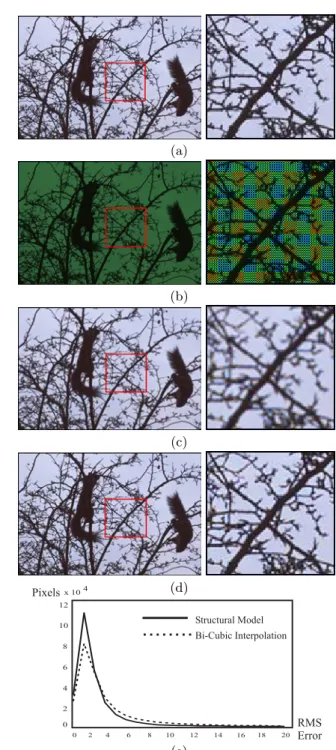
The above structural model was used to interpolate 20 test SVC images that are different from the ones used for training. In Figure 7(a), a high quality (8-bits per color channel) image is shown. Figure 7(b) shows the corresponding (downgraded) SVC image. This is really a single channel 8-bit image and its pixels are shown in color only to illustrate the Bayer pattern. Figure 7(c) shows a color image computed from the SVC image using bi-cubic interpolation. As is usually done, the three channels are interpolated separately using their respective data in the SVC image. The magnified image region clearly shows that bi-cubic interpolation results in a loss of high frequencies; the edges of the tree branches and the squirrels are severely blurred. Figure 7(d) shows the result of applying structural interpolation. Note that the result is of high quality with minimal loss of details.
(a) (b) (c) (d) 0 2 4 6 8 10 12 14 16 18 20 0 2 4 6 8 10 12 x 104 Structural Model Bi-Cubic Interpolation Pixels RMS Error (e)
Fig. 7. (a) Original (high quality) color image with 8-bits per color channel. (b) SVC image obtained by downgrading the original image. The pixels in this image are shown in color only to illustrate the Bayer mosaic. Color image computed from the SVC image using (c) bi-cubic interpolation and (d) structural interpolation. (e) Histograms of luminance error (averaged over 20 test images). The RMS error is 6.12 gray levels for bi-cubic interpolation and 3.27 gray levels for structural interpolation.
We have quantitatively verified of our results. Figure 7(e) shows histograms of the luminance error for bi-cubic and structural interpolation. These histograms are computed using all 20 test images (not just the one in Figure 7). The difference between the two histograms may appear to be small but is significant because a large fraction of the pixels in the 20 images belong to “flat” image regions that are easy to interpolate for both methods.The RMS errors (computed over all 20 images) are 6.12 and 3.27 gray levels for bi-cubic and structural interpolation, respectively.
5
Spatially Varying Exposures (SVE)
In [NM00], it was shown that the dynamic range of a gray-scale image detector can be significantly enhanced by assigning different exposures (neutral density filters) to pixels, as shown in Figure 8. This is yet another example of a multi-sampled image and is referred to as a spatially varying exposure (SVE) image. In [NM00], standard bi-cubic interpolation was used to reconstruct a high dynamic range gray-scale image from the captured SVE image; first, saturated and dark pixels are eliminated, then all remaining measurements are normalized by their exposure values, and finally bi-cubic interpolation is used to find the brightness values at the saturated and dark pixels. As expected, the resulting image has enhanced dynamic range but lower spatial resolution. In this section, we apply structural interpolation to SVE images and show how it outperforms bi-cubic interpolation. e e e e 1 4 3 2 p4 p3 p1 p2
Fig. 8.The dynamic range of an image detector can be improved by assigning different exposures to pixels. In this special case of 4 exposures, any 6×6 neighborhood in the image must belong to one of four possible sampling patterns shown asp1. . .p4.
5.1 SVE Structural Model
As in the SVC case, let the measured SVE data be M and the corresponding high dynamic range data be H. If the SVE detector uses only four discrete exposures (see Figure 8), it is easy to see that a neighborhood of any given size can have only one of four different sampling patterns (P = 4). Therefore, for each sampling patternp, a polynomial structural model is used that relates the captured data Mp within the neighborhood to the high dynamic range value
Hpat the center of the neighborhood:
Hp(i+ 0.5, j+ 0.5) = (x,y)∈Sp(i,j) Np n=0 Cp(a, b, n) Mpn(x, y), (7)
where, as before, (a, b) = (x−i, y−j), Sp(i, j) is the neighborhood of pixel (i, j),Np is the order of the polynomial mapping, andCp are the polynomial coefficients for the pattern p. Note that there is only one channel in this case (gray-scale) and hence the parameterλis omitted. The above model is rewritten in terms of a measurement matrix Ap and a reconstruction vector Hp, and the coefficients Cp are found using (5). The number of coefficients in the SVE structural model is determined as:
|C|=P+u∗v∗ P
p=1
Np. (8)
In our implementation, we have used P = 4, Np = 2 and u = v = 6, which given a total of 292 coefficients. SinceP = 4, only 73 coefficients are needed for reconstructing each pixel in the image.
5.2 Experiments
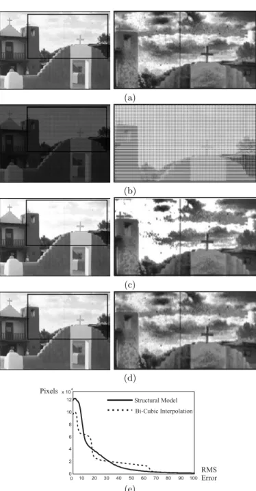
The SVE structural model was trained using 12-bit gray-scale versions of 6 of the images shown in Figure 3 and their corresponding 8-bit SVE images. Each SVE image was obtained by applying the exposure pattern shown in Figure 8 (withe4 = 4e3= 16e2= 64e1) to the original image, followed by a downgrade from 12 bits to 8 bits. The structural model was tested using 6 test images, one of which is shown in Figure 9. Figure 9(a) shows the original 12-bit image, Figure 9(b) shows the downgraded 8-bit SVE image, Figure 9(c) shows a 12-bit image obtained by bi-cubic interpolation of the SVE image, and Figure 9(d) shows the 12-bit image obtained by structural interpolation. The magnified images shown on the right are histogram equalized to bring out the details (in the clouds and walls) that are lost during bi-cubic interpolation but extracted by structural interpolation. Figure 9(e) compares the error histograms (computed using all 6 test images) for the two cases. The RMS errors were found to be 33.4 and 25.5 gray levels (in a 12-bit range) for bi-cubic and structural interpolations, respectively. Note that even though a very small number (6) of images were used for training, our method outperforms bi-cubic interpolation.
6
Spatially Varying Exposure and Color (SVEC)
Since we are able to extract high spatial and spectral resolution from SVC images and high spatial and brightness resolution from SVE images, it is natural to explore how these two types of multi-sampling can be combined into one. The result is the simultaneous sampling of space, color and exposure (see Figure 10). We refer to an image obtained in this manner as a spatially varying exposure and color (SVEC) image. If the SVEC image has 8-bits at each pixel, we would like to compute at each pixel three color values, each with 12 bits of precision. Since the same number of pixels on a detector are now being used to sample three different dimensions, it should be obvious that this is a truly challenging interpolation problem. We will see that structural interpolation does remarkably well at extracting the desired information.
(a) (b) (c) (d) RMS Error Pixels 0 10 20 30 40 50 60 70 80 90 100 0 2 4 6 8 10 12 x 104 Structural Model Bi-Cubic Interpolation (e)
Fig. 9. (a) Original 12-bit gray scale image. (b) 8-bit SVE image. (c) 12-bit (high dynamic range) image computed using bi-cubic interpolation. (d) 12-bit (high dynamic range) image computed using structural models. (d) Error histograms for the two case (averaged over 6 test images). The RMS error for the 6 images are 33.4 and 25.5 gray levels (on a 12-bit scale) for bi-cubic and structural interpolation, respectively. The magnified image regions on the right are histogram equalized.
R G R G R G R G R G R G R G R G R G R G R G R G G B G B G B G B G B G B G B G B G B G B G B G B R G R G R G R G G B G B G B G B R G R G R G R G R G R G R G R G R G R G R G R G R G R G R G R G R G R G R G R G R G R G R G R G R G R G R G R G R G R G R G R G R G R G R G R G G B G B G B G B G B G B G B G B G B G B G B G B G B G B G B G B G B G B G B G B G B G B G B G B G B G B G B G B G B G B G B G B G B G B G B G B R G R G R G R G R G R G R G R G R G R G R G R G G B G B G B G B G B G B G B G B G B G B G B G B p9 p10 p5 p1 p6 p2 p7 p3 p8 p12 p16 p11 p4 p13 p14 p15
Fig. 10.A combined mosaic of 3 spectral and 4 neutral density filters used to simulta-neously sample space, color and exposures using a single image detector. The captured 8-bit SVEC image can be used to compute a 12-bit (per channel) color image by structural interpolation. For this mosaic, for any neighborhood size, there are only 16 distinct sampling patterns. For a 4×4 neighborhood size, the patterns arep1. . .p16. Color and exposure filters can be used to construct an SVEC sensor in many ways. All possible mosaics that can be constructed fromΛcolors andEexposures are derived in [Aut01]. Here, we will focus on the mosaic shown in Figure 10, where 3 colors and 4 exposures are used. For any given neighborhood size, it is shown in [Aut01] that only 16 different sampling patterns exist (see Figure 10).
6.1 SVEC Structural Model
The polynomial structural model used in the SVEC case is the same as the one used for SVC, and is given by (3). The only caveat is that in the SVEC case we need to ensure that the neighborhood size used is large enough to adequately sample all the colors and exposures. That is, the neighborhood size is chosen such that it includes all colors and all exposures of each color.
The total number of polynomial coefficients needed is computed the same way as in the SVC case and is given by (6). In our experiments, we have used the mosaic shown in Figure 10. Therefore,P= 16,Λ= 3 (R,G, andB),Np= 2 for each of the 16 patterns, andu=v = 6, to give a total of 3504 coefficients. Once again, at each pixel, for each color, only 3504/48 = 73 coefficients are used. Therefore, even for this complex type of multi-sampling, our structural models can be applied to images in real-time using a set of linear filters.
6.2 Experiments
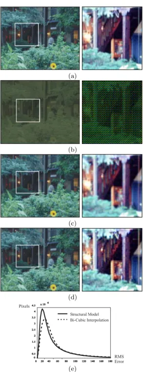
The SVEC structural model was trained using 6 of the images in Figure 3. In this case, the 12-bit color images in the training set were downgraded to 8-bit SVEC images. The original and SVEC images were used to compute the 3504 coefficients of the model. The model was then used to map 10 different test SVEC images to 12-bit color images. One of these results is shown in Figure 11. The original 12-bit image shown in Figure 11(a) was downgraded to obtain the 8-bit SVEC image shown in Figure 11(b). This image has a single channel
(a) (b) (c) (d) RMS Error Pixels 0 20 40 60 80 100 120 140 160 180 0 0.5 1 1.5 2 2.5 3 3.5 4 4.5 x 10x 104 Structural Model Bi-Cubic Interpolation (e)
Fig. 11. (a) Original 12-bit color image. (b) 8-bit SVEC Image. 12-bit color images reconstructed using (c) bi-cubic interpolation and (d) structural interpolation. (e) Lu-minance error histogram computed using 10 test images. RMS luLu-minance errors were found to be 118 and 80 (on a 12-bit scale) for bi-cubic and structural interpolation, respectively. The magnified images on the right are histogram equalized.
and is shown here in color only to illustrate the effect of simultaneous color and exposure sampling. Figures 11(c) and (d) show the results of applying bi-cubic and structural interpolation, respectively. It is evident from the magnified images on the right that structural interpolation yields greater spectral and spatial resolution. The two interpolation techniques are compared in Figure 11(e) which shows error histograms computed using all 10 test images. The RMS luminance errors were found to be 118 gray-levels and 80 gray-levels (on a 12 bit scale) for bi-cubic and structural interpolations, respectively.
Acknowledgements:This research was supported in parts by a ONR/ARPA MURI Grant (N00014-95-1-0601) and an NSF ITR Award (IIS-00-85864).
References
[Aut01] Authors. Resolution Enhancement Along Multiple Imaging Dimensions Using Structural Models. Technical Report, Authors’ Institution, 2001.
[Bay76] B. E. Bayer. Color imaging array. U.S. Patent 3,971,065, July 1976. [BE00] M. Ben-Ezra. Segmentation with Invisible Keying Signal. InCVPR, 2000. [BK00] S. Baker and T. Kanade. Limits on Super-Resolution and How to Break
Them. InProc. of CVPR, pages II:372–379, 2000.
[Bra65] R. N. Bracewell. The Fourier Transform and Its Applications. McGraw Hill, 1965.
[Bra94] D. Brainard. Bayesian method for reconstructing color images from trichro-matic samples. In Proc. of IS&T 47th Annual Meeting, pages 375–380, Rochester, New York, 1994.
[Dil77] P. L. P. Dillon. Color imaging array. U.S. Patent 4,047203, September 1977. [Dil78] P. L. P Dillon. Fabrication and performance of color filter arrays for solid-state imagers. In IEEE Trans. on Electron Devices, volume ED-25, pages 97–101, 1978.
[DM97] P. Debevec and J. Malik. Recovering High Dynamic Range Radiance Maps from Photographs. Proc. of ACM SIGGRAPH 1997, pages 369–378, 1997. [FP99] W. Freeman and E. Pasztor. Learning Low-Level Vision. InProc. of ICCV,
pages 1182–1189, 1999.
[GHZ92] R. Ginosar, O. Hilsenrath, and Y. Zeevi. Wide dynamic range camera. U.S. Patent 5,144,442, September 1992.
[KM85] K. Knop and R. Morf. A new class of mosaic color encoding patterns for single-chip cameras. In IEEE Trans. on Electron Devices, volume ED-32, 1985.
[MN99] T. Mitsunaga and S. K. Nayar. Radiometric Self Calibration. In Proc. of CVPR, pages I:374–380, 1999.
[MOS83] D. Manabe, T. Ohta, and Y. Shimidzu. Color filter array for IC image sensor. InProc. of IEEE Custom Integrated Circuits Conference, pages 451–455, 1983. [MP95] S. Mann and R. Picard. Being ‘Undigital’ with Digital Cameras: Extending Dynamic Range by Combining Differently Exposed Pictures. Proc. of IST’s 48th Annual Conf., pages 442–448, May 1995.
[NM00] S. K. Nayar and T. Mitsunaga. High Dynamic Range Imaging: Spatially Varying Pixel Exposures. InProc. of CVPR, pages I:472–479, 2000. [Par85] K. A. Parulski. Color filters and processing alternatives for one-chip cameras.
InIEEE Trans. on Electron Devices, volume ED-32, 1985.
[SN01] Y. Y. Schechner and S. K. Nayar. Generalized mosaicing. InICCV, 2001. [WS95] M. A. Wober and R. Soini. Method and apparatus for recovering image data