Selection of the Number of Principal Components: The Variance of the Reconstruction Error Criterion with a Comparison to Other Methods

Selection of the Number of Principal Components: The Variance of

the Reconstruction Error Criterion with a Comparison to Other

Methods

†

Sergio Valle, Weihua Li, and S. Joe Qin*

Department of Chemical Engineering, The University of Texas at Austin, Austin, Texas 78712

One of the main difficulties in using principal component analysis (PCA) is the selection of the number of principal components (PCs). There exist a plethora of methods to calculate the number of PCs, but most of them use monotonically increasing or decreasing indices. Therefore, the decision to choose the number of principal components is very subjective. In this paper, we present a method based on the variance of the reconstruction error to select the number of PCs. This method demonstrates a minimum over the number of PCs. Conditions are given under which this minimum corresponds to the true number of PCs. Ten other methods available in the signal processing and chemometrics literature are overviewed and compared with the proposed method. Three data sets are used to test the different methods for selecting the number of PCs: two of them are real process data and the other one is a batch reactor simulation.

1. Introduction

Principal component analysis (PCA) has wide ap-plications in signal processing,1_{factor analysis,}2 chemo-metrics,3 _{and chemical processes data analysis.}4,5 Al-though the original concept of PCA was introduced by Pearson33_{and developed by Hotelling,}32_{the vast} major-ity of applications happened only in the last few decades with the popular use of computers. In the chemical engineering area. the applications of PCA include the following:

(1) monitoring of batch and continuous processes,6,7 (2) extraction of active biochemical reactions,8₍₃₎ prod-uct quality control in the principal component subspace,9 (4) missing value replacement10_{(5) sensor fault} identi-fication and reconstruction,11_{(6) process fault} identifica-tion and reconstrucidentifica-tion,12 _{and (7) disturbance} detec-tion.13_{Early PCA applications to the quality control of} chemical processes are documented in Jackson.4

A key issue in developing a PCA model is to choose the adequate number of PCs to represent the system in an optimal way. If fewer PCs are selected than required, a poor model will be obtained and an incomplete representation of the process results. On the contrary, if more PCs than necessary are selected, the model will be overparameterized and will include noise. Zwick and Velicer20_{compared five different approaches available} in the literature. Himes et al.34 _{provide further} com-parisons of several approaches using the Tennessee Eastman problem. Different approaches had been pro-posed in the past to select the optimal number of PCs: (1) Akaike information criterion (AIC),14_{(2) minimum} description length (MDL),15_{(3) imbedded error function} (IEF),16_{(4) cumulative percent variance (CPV),}2_{(5) scree} test on residual percent variance (RPV),17,18_{(6) average} eigenvalue (AE),19_{(7) parallel analysis (PA),}20₍₈₎ au-tocorrelation (AC),21 _{(9) cross validation based on the}

PRESS and R ratio,3,22,23 _{and (10) variance of the} reconstruction error (VRE).29

In the signal processing literature, PCA has been used to determine the number of independent source signals from noisy observations by selecting the number of significant principal components.1 _{Under the} assump-tion that measurement noise corresponds to the smallest equal eigenvalues of the covariance matrix, the Akaike information criterion and the minimum description length principle have been applied to selecting the number of PCs.1_{These criteria apply to PCA based on} the covariance matrix of the data and do not work on the correlation-based PCA of the data, although cor-relation-based PCA is preferred in chemical processes to equally weight all variables by variance scaling. One advantage of the AIC and MDL criteria is that they have a solid statistical basis and are theoretically shown to have a minimum number of PCs.

To develop a selection criterion that works with both correlation-based and covariance-based PCA, Qin and Dunia29 _{propose a new criterion to determine the} number of PCs based on the best reconstruction of the variables. An important feature of this new approach is that the proposed index has a minimum (i.e.. non-monotonic) corresponding to the best reconstruction. When the PCA model is used to reconstruct missing values or faulty sensors, the reconstruction error is a function of the number of PCs. Qin and Dunia29_{use the}

variance of the reconstruction error to determine the

number of PCs. The VRE can be decomposed into a portion in the principal component subspace (PCS) and a portion in the residual subspace (RS). The portion in the RS is shown to decrease monotonically with the number of PCs and that, in the PCS in general, increases with the number of PCs. As a result, the VRE always has a minimum which points to the optimal number of PCs for best reconstruction. In the case of missing value reconstruction, the VRE for different missing patterns are combined with weights based on the frequency of occurrence. In the case of faulty sensor identification and reconstruction, the VREs are weighted based on the variance of each variable. In the special

* To whom correspondence should be addressed. Tel: (512)-471-4417. Fax: (512)471-7060. E-mail: [email protected]. †_{An earlier version of the paper was presented at the AIChE} Annual Meeting, Miami, FL, Nov 16-20, 1998.

4389 Ind. Eng. Chem. Res. 1999, 38, 4389 4401

10.1021/ie990110i CCC: $18.00 © 1999 American Chemical Society

case where each sensor is reconstructed once, the procedure can be thought of as a cross validation by

leaving sensors out, in contrast to the traditional leaving samples out cross validation.

The ultimate purpose of this paper is 3-fold:

(1) Introduce the VRE, AIC, MDL, and other related methods for the selection of the number of principal components in chemical process data modeling. (2) Provide further analysis and comparison of the

VRE method with other methods, including the AIC and MDL criteria.

(3) Compare and benchmark various methods for selecting the number of PCs using data from a simulated batch reactor and two industrial pro-cesses data sets. The effectiveness of these methods will be tested and bench-marked on the basis of these data sets.

The organization of the paper is given as follows. Section 2 describes the selection criteria based on AIC, MDL, and IEF methods. Section 3 describes different selection criteria commonly used in the PCA literature. Section 4 presents the VRE method based on the correlation matrix and covariance matrix. Section 5 compares the methods using three examples: a simu-lated batch reactor, a boiler process, and an incineration process. Section 6 concludes the paper.

2. Criteria Based on AIC, MDL, and IEF

The AIC and MDL criteria are popular in signal processing, while the IEF approach is proposed in factor analysis.16_{Although these three methods are developed} in different areas. There are common attributes about them: (1) they work only with covariance-based PCA; (2) the variances of measurement noise in each variable are assumed to be identical; and (3) they demonstrate a minimum over the number of PCs given the above assumptions.

In this section, we first present the notation and basic relations for PCA. Then we provide a linkage between the use of PCA for signal processing and the use of PCA for process modeling. Finally, the criteria for AIC, MDL, and IEF are presented.

2.1. PCA Notation. Let x ∈ Rm _{denote a sample} vector of m sensors. Assuming that there are N samples for each sensor, a data matrix X∈ RN×m_{is composed} with each row representing a sample. The matrix X is scaled to zero-mean for covariance-based PCA and, in addition to unit variance for correlation-based PCA, by either the NIPALS24_{or a singular-value decomposition} (SVD) algorithm. The matrix X can be decomposed into a score matrix T and a loading matrix P whose columns are the right singular vectors of X,

where X˜ ) T˜P˜T _{is the residual matrix. Since the} columns of T are orthogonal, the covariance matrix is

where

and tiis the ith column of T andλiare the eigenvalues of the covariance matrix. If N is very large, the ap-proximate equality in eq 2 becomes an equality. We assume the equality holds in this paper unless otherwise specified. For variance scaled X, eq 2 is the correlation matrix R.

A sample vector x can be projected on the PCS (Sp), which is spanned by P∈Rm×l_{, and RS (Sr), respectively,}

Since Spand Srare orthogonal,

and

The task for determining the number of PCs is to choose

l such that xˆ contains mostly information and xˆ contains noise.

2.2. PCA for Signal Processing and Process Modeling. In signal processing, PCA has been used to

detect q independent signal sources from m observation variables, that is,

where x(k) ∈Rm_{is a vector of observation variables,}

s(k) ∈_Rq_{is a vector of signal sources, n(k)∈ R}m_{is a} vector of observation noise, and A∈_Rm×q _{is a matrix} with appropriate dimension. This model is used for radar signal detection,1_{for instance.}

In chemical process modeling, the physical principles that govern the process behavior are mainly material and energy balances. Assuming there exists a linear (or linearized) relationship among the process variables, the following steady-state relation can be derived,

where xj(k) ∈_Rm_{are the true process variables free of} measurement noise, B∈Rq˜×m_{is the model matrix, and}

n(k)∈Rm_{is the measurement noise.}

While eqs 9 and 11 represent different physical phenomena, we have the following remarks under the condition that q)m-q˜:

(1) Equation 9 can be converted to eqs 10 and 11 by premultiplying

on both sides of eq 9, where

(2) Equation 11 can be converted to eq 9 by selecting

A as a basis in R(BT_{), where R(B}T_{) is the range} space of BT_.

On the basis of the equivalence of eqs 9 and 11, we can directly apply AIC and MDL criteria originally

λi) 1 N-1ti T ti)var{ti} (4) xˆ )PPTx∈S_p (5) x˜ )P˜P˜Tx)(I-PPT) x∈Sr (6) xˆTx˜ )0 (7) xˆ +x˜ )x (8) x(k))As(k)+n(k) (9) Bxj(k))0 (10) x(k))xj(k)+n(k) (11) B)[I-A(ATA)-1AT] (12) xj(k))x(k)-n(k))As(k) X)TPT+X˜ )TPT+T˜P˜T)[T T˜][P P˜]T (1) S≈ 1 N-1X T X)[P P˜]Λ[P P˜]T (2) Λ) 1 N-1[T T˜] T [T T˜])diag{λ1,λ2,‚‚‚,λm} (3)

proposed for the detection of signal sources in signal processing1_{to the determination of the number of PCs} in process modeling.

2.3. AIC and MDL Criteria. AIC and MDL are

respectively proposed by Akaike14_{and Rissanen}15 _for model selection. Assuming that n(k) ∼ N(0, σ2_{I) is} independently identically distributed, we can describe the covariance matrix of x(k) in the following form,

where Sh )E{xjxjT_{) has a rank q}

em.

Denoting the eigenvalues of S byλ1gλ2,‚‚‚,gλm, it

is easy to verify that the smallest m-q eigenvalues of S are equal toσ2_{, that is,}

and

where λ1, ‚‚‚, λq and v1, ‚‚‚, vq are the q largest eigenvalues and the associated eigenvectors of S. We denote

as the parameter vector for the PCA model. Wax and Kailath1_{propose to determine the number of PCs based} on AIC and MDL, which can be summarized as follows. Given a set of N observations x(1),‚‚‚, x(N), which are assumed to be a sequence of independent and identically distributed zero-mean Gaussian vectors, the maximum likelihood estimate of w1,25_{is given by}

where d1,‚‚‚, dmare the eigenvalues and c1,‚‚‚, clthe eigenvectors of the sample covariance matrix, which is

Sˆ ) 1/(N - 1)∑_k)1

N _x(k)xT_{(k). Wax and Kailath}1 _have shown that the AIC and MDL functions will have the following forms,

where M is the number of independent parameters in the model vector wˆ . For complex valued signals, the eigenvectors c1, c2,‚‚‚, clare complex, and the number of independent parameters is1

For real valued signals such as those encountered in chemical processes, the eigenvectors c1, c2, ‚‚‚, cl are real. Since these vectors are normalized and mutually orthogonal, the number of independent parameters in these eigenvectors is

This formula is used for the application examples in this paper.

The first term in AIC(l) or MDL(l) tends to decrease and the second term increases with l. Theoretically, a minimum results for l∈[1, m]. Wax and Kailath1_show that, for a large data length N, MDL gives a consistent estimate, while AIC tends to overestimate the number of PCs.

2.4. Imbedded Error Function. The IEF method16 is based on the idea that the measurement space can be divided in two subspaces: a principal component sub-space which represents the important signals of the process and a residual subspace that has only noise in its measurements. The only requirement to calculate this function is to know the eigenvalues. The calculation of this function is done using only the residual eigen-values:

where l represents the number of PCs used to represent the data. The IEF method assumes that the data contain signals plus measurement errors similar to those in eq 11. Each PC will contain a portion of the signals and a portion of imbedded errors. Before all signals are extracted, the IEF(l) contains a mixture of signal and imbedded errors, which tends to decrease with l. At the point all signals are extracted, the IEF(l) contains imbedded errors only and should increase with

l. The minimum value of the IEF, if exists, corresponds

to the number of PCs needed to describe the data by leaving out measurement errors only.

3. Selection Criteria in Chemometrics

3.1. Cumulative Percent Variance. The CPV2_{is a} measure of the percent variance captured by the first l PCs:

With this criterion one selects a desired CPV, e.g., 90%, 95%, or 99%, which is very subjective. While we would like to account for as much of the variance as possible, we want to retain as few principal components as possible. The decision then becomes a balance between the amount of parsimony and comprehensiveness of the model. We must decide what balance will serve our purpose. The CPV method to select the number of PCs is often ambiguous because the CPV is monotonically increasing with the number of PCs.

M) l 2(m-l+1) IEF(l))

[

l

∑

j)l+1 m λj Nm(m-l)

]

1/2 (16) CPV(l))100

[

∑

j)1 l λj

∑

j)1 m λj

]

% (17) S)E{xxT})Sh +σ2I (13) λq+1)λq+2) ‚‚‚ )λm)σ 2 S)

∑

i)1 q (λi-σ 2 )vivi T₊ σ2I w)[λ1,‚‚‚,λq,σ 2 , v1 T ,‚‚‚, vq T ]T∈R(m+1)q+1 wˆ )

[

d1,‚‚‚, dl, 1 m-li)

∑

l+1 m di, c1 T ,‚‚‚, cl T

]

T AIC(l)) -2 log

(

∏

s)l+1 m ds 1/(m-l) 1 m-ls)

∑

l+1 m ds

)

(m-l)N +_{2M (14)} MDL(l)) -2 1og

(

∏

s)l+1 m ds 1/(n-l) 1 m-ls)

∑

l+1 m d_s

)

(m-l)N +_{M log N} (15) M)l(2m-l)

3.2. Scree Test on Residual Percent Variance.

The Scree test on RPV17,18_{is an empirical procedure to} select the number of PCs using the RPV as a basis. The method looks for a “knee” point in the residual percent

variance plotted against the number of principal

com-ponents. The method is based on the idea that the residual variance should reach a steady state when the factors begin to account for random errors. When a break point is found or when the plot stabilizes, that point corresponds to the number of principal compo-nents to represent the process. The RPV uses only the residual eigenvalues to do the calculations:

The implementation of this method is relatively easy, but in some cases it is difficult to find a knee if the curve decreases smoothly. This point is observed in section 5.3 of the paper using the incineration process data.

3.3. Average Eigenvalue. The average eigenvalue

approach19 _{is a somewhat popular criterion to choose} the number of PCs. This criterion accepts all eigenval-ues with valeigenval-ues above the average eigenvalue and rejects those below the average. The reason is that a PC contributing less than an “average” variable is insignificant. For covariance-based PCA, the average eigenvalue is1_{/mtrace(S), and for correlation-based PCA} the average eigenvalue1_{/mtrace(R), which is 1. Then} all the eigenvalues above 1 will be selected as the principal eigenvalues to form the model. Therefore, this criterion is also known as the eigenvalue-one rule.

3.4. Paralle1 Analysis. The PA method basically

builds PCA models for two matrices: one is the original data matrix and the other is an uncorrelated data matrix with the same size as the original matrix. This method was developed originally by Horn26_{to enhance} the performance of the Scree test. When the eigenvalues for each matrix are plotted in the same figure, all the values above the intersection represent the process information and the values under the intersection are considered noise. Because of this intersection, the paral-lel analysis method is not ambiguous in the selection of the number of PCs.

For a large number of samples, the eigenvalues for a correlation matrix of uncorrelated variables are 1. In this case, the PA method is identical to the AE method. However, when the samples are generated with a finite number of samples, the initial eigenvalues exceed 1, while the final eigenvalues are under 1. That is why Horn26 _{suggested comparing the correlation matrix} eigenvalues for uncorrelated variables with those of a real data matrix based on the same sample size.

3.5. Autocorrelation. According to Shrager and

Hendler,21 _{it is possible to use an autocorrelation} function to separate the noisy eigenvectors from the smooth ones using either the score matrix or the loading matrix. A simple statistic for detecting noise is the autocorrelation function of order 1 for the PCA scores,

where N represents the number of samples. A value greater than+0.5 indicates smoothness of the scores, while a value smaller than 0.5 indicates that the component contains mainly noise and should not be included in the model.21_{Two major drawbacks of this} method are (1) this 0.5 threshold is somewhat arbitrary and (2) a large variance PC can have little autocorre-lation. The second drawback is observed in the incinera-tion data in secincinera-tion 5 of this paper.

3.6. Cross Validation Based on the R Ratio. Cross

validation3,27_{is a popular statistical criterion to choose} the number of factors in PCA. The basis of this method is to estimate the values of some deleted data from a model and then compare these estimates with the actual values. Wold3_{proposes a cross-validation method known} as the R ratio. This method randomly divides the data set X into G groups. Then, for a starting value of l)1, a reduced data set is formed by deleting each group in turn and the parameters in the model are calculated from the reduced data set. The predicted error sum of squares (PRESS) is calculated from the predicted and actual values of the deleted objects. In the meantime, the residual sum of squares (RSS) the next component is extracted is calculated. A ratio,

is then calculated starting with l)1,‚‚‚, m-1. A value of the R ratio less than 1 indicates that the newly added component in the model improved the prediction and hence the calculation proceeds. A value of this ratio larger than 1 indicates that the new component does not improve the prediction and hence should be deleted. Since the PCA model calculation involves randomly deleted data, the NIPALS algorithm is used which can handle missing values. The brief procedure for calculating the R ratio is summarized as follows. Refer to Wold3_{for the detailed procedure.}

(1) Scale the data X to zero-mean (and unit variance for correlation-based PCA). Set l)1 and X0)X.

(2) Calculate:

(3) Divide Xl-1 randomly into G groups. For all but one group calculate the lth PCA factor using the NIPALS algorithm that handles missing values. After leaving out each group in turn. calculate PRESS(l) for all groups of data.

(4) Calculate the R ratio using eq 20. If R<1, then calculate the lth PCA factor based on all data Xl-1,

set Xl )Xl-1 -tlpl T

, set l :)l+ 1, and return to step 2. If R _g1, terminate the program.

3.7. Cross Validation Based on PRESS. In the R ratio method, the PRESS is calculated in a manner that Xl-1may be rerandomized after each increment of l. If a new PC results in a PRESS that is larger than the RSS without this PC, it is discarded. An alternative approach is to use PRESS alone to determine the number of PCs. This procedure is related to Wold3_and has been successfully used in practice.28_{The procedure} to use PRESS to determine the number of PCs is summarized as follows:

(1) Scale the data X to zero-mean (and unit variance for correlation-based PCA). Set l)1.

R(l)) PRESS(l) RSS(l-1) (20) RSS(l-1))trace(Xl-1 T Xl-1) RPV(l))100

[

∑

j)l+1 m λj

∑

j)1 m λj

]

% (18) AC(l))

∑

i)1 N-1 t_i,lt_i+1,l (19)

(2) Divide X randomly into G groups. For all but one group calculate all PCA factors using the NIPALS algorithm that handles missing values. After leav-ing out each group in turn, calculate PRESS(l) for all groups of data.

(3) A minimum in PRESS(l) corresponds to the best number of PCs to choose.

Note that the number of PCs calculated in this procedure can be different from that in the method of the R ratio.

4. Variance of the Reconstruction Error Criterion

The variance of the reconstruction error method was developed by Qin and Dunia29_{to select the number of} principal components based on the best reconstruction of the variables. An important characteristic of this approach is that the VRE index has a minimum, corresponding to the best reconstruction. When the PCA model is used to reconstruct missing values or faulty sensors, the reconstruction error is a function of the number of PCs. The minimum found in the VRE calculation directly determines the number of PCs. This is because the VRE is decomposed in two subspaces: the principal components subspace and a residual subspace. The portion in PCS has a tendency to increase with the number of PCs, and that in the RS has a tendency to decrease, resulting in a minimum in VRE.

Qin and Dunia29_{consider that the sensor} measure-ment is corrupted with a fault along a directionξi,

where x* is the normal portion, f the fault magnitude, and_|ξi|)1. For sensor faults,ξicorresponds to the ith

column of an identity matrix. For process faults,ξican be an arbitrary vector with unit norm. The reconstruc-tion of the fault is given by correcreconstruc-tion along the fault direction, that is,

so that xiis most consistent with the PCA model. The difference x*-xiis known as the reconstruction error. Qin and Dunia29_{define the variance of the} reconstruc-tion error as

where

The problem to find the number of PCs is to mini-mize uiwith respect to the number of PCs. Considering all possible faults, the VRE to be minimized is defined as

The variance-based weighting factors are necessary to equalize the importance of each variable. Note that the

above derivation is for a correlation-based PCA sincethe correlation matrix R is used. For a covariance-based PCA, one can simply replace with S the covariance matrix.

The VRE procedure for selecting the number of PCs can be summarized as follows:

(1) Build a PCA model using normal data from all variables.

(2) Reconstruct each variable using other variables and calculate the VRE, ui.

(3) The total VRE is calculated using eq 23.

(4) The number of PCs that gives the minimum VRE is selected, which corresponds to the best recon-struction.

For a particular variable or fault direction ξi, it is possible that ui _g var{ξT_x}_{, which means the model} gives a worse prediction than the mean of the data. In this case, the variable has little correlation with others and should be dropped from the model. There-fore, the VRE can be used to achieve the following objectives: (1) determine the number of PCs by leaving out variables; (2) select variables that can be reliably reconstructed from the model; (3) simultaneously leave out a group of variables; and (4) include a particular fault or disturbance direction in selecting the num-ber of PCs for the purpose of fault or disturbance detection.

4.1. VRE versus PRESS. Like PRESS, the VRE

method works for both a correlation-based PCA and covariance-based PCA. Another similarity between VRE and PRESS is that they do not require any fault to occur; they just need to leave out a portion of the data and reconstruct them from the models. Furthermore, the missing value treatment in the NIPALS algorithm is equivalent to the fault reconstruction as shown in Dunia et al.11_{However, the VRE and PRESS methods} are different in the following ways:

(1) The VRE method can include process faults with arbitrary directionξito emphasize particular pro-cess faults or disturbances, while PRESS cannot. (2) If each sensor direction (ξi) is used once and only once, the VRE method is similar to cross validation by leaving sensors out, while the PRESS leaves samples out randomly.

(3) In PRESS, as many as G models are built in the presence of “missing” values, while VRE builds one PCA model only based on all available data. (4) In the VRE method, it is possible to check if a

group of data can be reliably reconstructed, while the PRESS method fails to do this rigorously. (5) The VRE method is also suitable for recursive

on-line calculation, as shown in Li et al.30

4.2. Consistency of the VRE Method. Wax and

Kailath1_{show that the MDL approach gives a consistent} estimate of the number of PCs, while the AIC method

x)x*+fξi x_i)x-f_iξi ui≡var{ξi T (x-xi)}) ξ ˜ i T Rξ˜i (ξ˜i T ξ˜i) 2 (21) ξ ˜ i)(I-PP T )ξ_i)P˜P˜Tξi (22) VRE(l))

∑

i)1 m _u i var{ξi T x} )

∑

i)1 m _u i ξi T Rξi (23)

does not and tends to overestimate the number of PCs. The consistency of most other methods are not known. For the VRE method, Dunia and Qin12_{show that the} VRE demonstrates a minimum, but it is not known whether the minimum corresponds to the true number of PCs. In this section, we establish the consistency conditions for the VRE method.

First, we examine the covariance-based PCA where the noise variances are assumed equal. From eq 13, the eigenvalues of covariance matrix S are

whereλhi(i)1, 2, ..., q) are the non-zero eigenvalues of

Sh, the covariance of xj. For convenience we requireλh1g

λ

h_2g‚‚‚_gλhq. Assuming l PCs are included in the PCA model, the VRE can be written as follows using eq 22,

where eil≡P˜_lTξi∈Rl_andΛ

l)diag{λl+1,λl+2,‚‚‚,λm}. Given the above analysis, we have the following theorem about the consistency of the covariance-based VRE method.

Theorem 1. Assuming the covariance matrix of the

data is given in eq 13, then (1) the VRE achieves a minimum at l _eq and (2) the VRE achieves a global

minimum at l)q ifλhqg |eil|2/|eiq|2σ2for l<q.

The proof of this theorem is given in Appendix A. We make the following remarks about Theorem 1:

(1) The VRE method will never over estimate the number of PCs.

Figure 2. Comparison for the simulated batch reactor free of noise.

λi)

{

λhi+σ 2 1eieq σ2 q<iem uil) ξ ˜ il T ξ˜il (ξ˜il T ξ˜il) 2) ξi T P˜_l(P˜_lTSP˜_l)P˜_lTξi (ξi T P˜lP˜l T ξi) 2 ≡ e_ilTP˜_lTSP˜_le_il (eil T eil) 2 ) e_ilTΛleil (e_ilTe_il)2 (24)

(2) The condition for a consistent estimate requires that the variance of the signal is slightly larger than the variance of the noise, which is quite reasonable.

For a correlation-based PCA or the general case of a covariance-based PCA, the measurement errors do not necessarily have the same variance. In this case, we denote the eigenvalues of the correlation (or covariance) matrix asλ1,λ2,‚‚‚,λq,σ_q+1

2 ,σ_q+2

2

,‚‚‚,σ_m2, whereσ_i2are variance quantities of the noise terms. To guarantee that VRE gives a consistent estimate in this case, we have the following theorem.

Theorem 2. Assuming the eigenvalues of the

cor-relation or covariance matrix with descending order are λ1,λ2,‚‚‚,λq,σq+1

2 _,‚‚‚, σm

2_{, the VRE achieves a minimum} at l)q if (1)σm

2

gσq+1 2

|eil|2/|eiq|2for lgq, and (2)λlg

σ_q+1 2 ₍₁₊

|eil|2/|eiq|2) for l<q.

The proof of this theorem is given in Appendix B. The first condition requires that the noise variances, al-though different, should not be too different. The second condition requires that the variance of the signal be larger than the variance of the noise.

5. Comparisons on Three Case Studies

5.1. Simulated Batch Reactor Data. An isothermal

batch reactor is simulated with four first-order reactions taking place.31 _{Figure 1 depicts the reaction network} for the batch reactor. The material balance equation for the batch reactor is

where the reaction rates for the five species are Figure 3. Comparison for the simulated batch reactor with stationary additive Gaussian noise.

dC_i

The reaction rate constants are

The temperature was kept constant at 334.6 °C. It was assumed that initially only the raw material A was present and the vessel was well-mixed. Three different cases of measurement noise were simulated for the batch reactor: (1) a noise-free case, (2) stationary additive Gaussian noise with a standard deviation of 0.002, and (3) nonstationary multiplicative Gaussian noise with a standard deviation of 10% of the variables amplitude.

The simulation generated a total of 200 samples for the 5 variables using this kinetic model. The data were scaled to zero-mean and unit variance, and then analyzed with the 11 different methods to determine the number of PCs to adequately represent the model. Figure 4. Comparison for the simulated batch reactor with nonstationary multiplicative Gaussian noise.

r_A) -k₁C_A-k₂C_A) -(k₁+k₂)C_A r_R)k₁C_A-k₃C_R-k₄C_R)k₁C_A-(k₃+k₄)C_R r_T)k₂C_A r_U)k₄C_R rS)k3CR k₁)107exp

{

-5000 T

}

[)]h -1 k₂)1.246×105exp

{

4000 T

}

[)]h -1 k3)10 10 exp

{

-9000 T

}

[)]h -1 k4)1.246×10 8 exp

{

-7000 T

}

[)]h -1

The analysis results are shown in Figure 2 for the noise-free case, Figure 3 for the additive noise, and Figure 4 for the case of multiplicative noise. Table 1

summarizes the results for the case of additive noise and shows if the method has found a solution, an ambiguous solution or no solution at all.

Observe that, for the additive noise case, the RPV method shows a smooth curve, making it difficult to decide on the number of PCs. The CPV and PRESS methods choose three PCs. AE and PA determine one PC, and the rest of the seven methods agree in two PCs. We conclude that to have an adequate representation of the process, it is necessary to use two PCs. Also observe in Figure 2 (noise-free) and Figure 4 (multipli-cative noise) that the AIC and MDL methods were unable to find a solution.

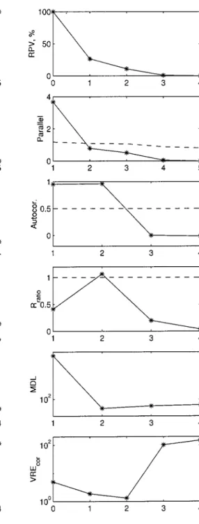
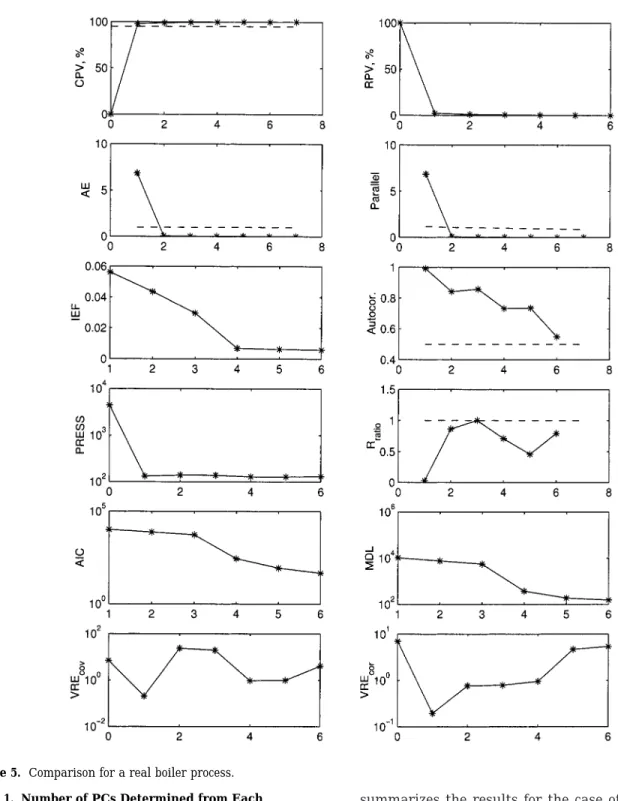
5.2. Boiler Process Data. The data from an

indus-trial boiler consist of 7 variables and 630 samples. The variables represent temperatures, pressures, flows, and concentrations. Before the analysis was done the data were centered and scaled to zero-mean and unit vari-Figure 5. Comparison for a real boiler process.

Table 1. Number of PCs Determined from Each Analyzed Method

reactor boiler incinerator

CPV 3 1 15

RPV ambiguous 1 ambiguous

AE 1 1 7

PA 1 1 7

IEF 2 no solution no solution

AC 2 no solution 2

PRESS 3 1 15

Rratio 2 2 5

AIC 2 no solution no solution

MDL 2 no solution no solution

VREcov 2 1 2

ance. The results from the 11 methods are shown in Figure 5, with the selected number of PCs shown in Table 1.

It is seen from Figure 5 that, for the CPV method, this process is highly correlated because only with one PC that one is able to capture more than 95% of the variance. Basically, all the methods that found a solu-tion agree with one PC with the excepsolu-tion of the R ratio method. The IEF, AIC, and MDL methods are unable to find a minimum for this real data set. The autocor-relation method is also ineffective.

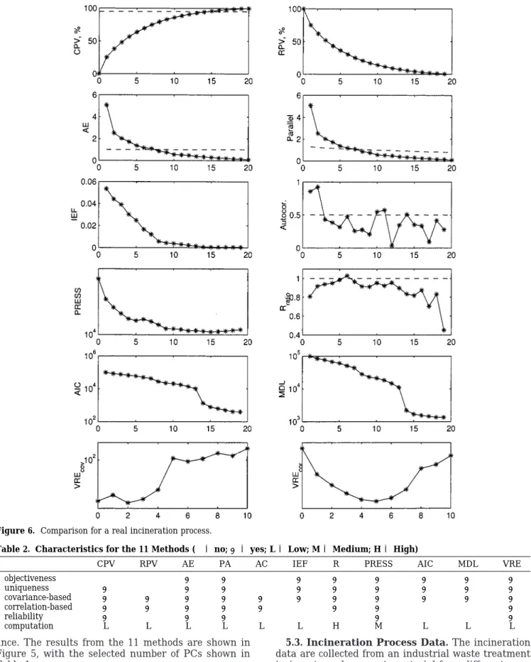
5.3. Incineration Process Data. The incineration

data are collected from an industrial waste treatment incinerator, where waste material from different reac-tions in a process are burned before they are released to the atmosphere. The total analyzed data are 900 samples and 20 variables. The variables included are temperatures, pressures, flows, and concentrations. Figure 6 depicts the results from the 11 methods, and Tables 1 and 2 summarize the selected number of PCs for each method and the characteristics for the 11 methods respectively.

Figure 6. Comparison for a real incineration process.

Table 2. Characteristics for the 11 Methods (_×)no;_x)yes; L)Low; M)Medium; H)High)

CPV RPV AE PA AC IEF R PRESS AIC MDL VRE

objectiveness _{× × x x × x x x x x x} uniqueness x × x x × x x x x x x covariance-based _{x x x x x x x x x x x} correlation-based x x x x x × x x × × x reliability x × x x × × × x × × x computation L L L L L L H M L L L

This process is very noisy and, as expected, the number of PCs to represent the process is large. The IEF, AIC, and MDL methods did not find a solution at all. The autocorrelation method is somewhat ambiguous as the autocorrelation of the 10th and 11th PCs become larger than 0.5 after several PCs being smaller than 0.5. The RPV index is monotonically decreasing but fails to show a knee location, making the solution ambiguous. The rest of the methods found a solution. However, the PRESS solution is too high and VREcovtoo low for this process. The R ratio and VREcor agree in the same solution.

6. Conclusions

Among the 11 methods presented in the paper, most of them have monotonically decreasing or increasing indices. The IEF, AC, AIC, and MDL worked well with the simulated example, but they failed when used with real data. The most reliable methods are CPV, AE, PA, PRESS, and VRE.

A comparison of the 11 tested methods for the selection of the number of PCs is summarized in Table 2. Considering the effectiveness, reliability, and objec-tiveness, the PRESS- and correlation-based VRE meth-ods are superior to the others. The VRE method is preferred to the PRESS method in the consistency of the estimate, computational cost, and ability to include a particular disturbance or fault direction in selecting the number of PCs.

Acknowledgment

This work is supported by the National Science Foundation (under Grant CTS-9814340), AMD, Air Products, ALCOA Foundation, DuPont, Union Carbide, Consejo Nacional de Ciencia y Tecnologı´a (CONACyT), and Instituto Tecnolo´gico de Durango (ITD).

Nomenclature

AC)autocorrelation index B)model matrix

C)model projection matrix Ci)component i concentration

CPV)cumulative percent variance index f)fault magnitude

I)identity matrix

IEF)imbedded error function index ki)reaction rate constant for component i

l)number of principal components m)number of variables

M)number of independent parameters n)observation noise vector

N)number of samples P)loadings matrix

PRESS)predicted error sum of squares index ri)reaction rate for component i

R)R ratio index R)correlation matrix

RPV)residual percent variance index RSS)residual sum of squares

E)expectation R)real

s)signal sources vector S)covariance matrix

Sp)principal components subspace Sr)residual subspace

t)score vector T)temperature T)score matrix

u)variance of the reconstruction error x)sample vector

X)data matrix Greek Letters

λ)eigenvalue ξ)fault direction

Λ)eigenvalues diagonal matrix |‚|)Euclidean norm

Superscripts and Subscripts

‚˜ )_{referred to the residual subspace}

‚ˆ )referred to the principal components subspace /)_{uncorrupted portion}

T)transpose Abbreviations AC)autocorrelation

CPV)cumulative percent variance diag)diagonal

IEF)imbedded error function PCA)principal components analysis PCS)principal components subspace PRESS)predicted sum of squares RS)residual subspace

RSS)residual sum of squares PCs)principal components RPV)residual percent variance

VRE)variance of the reconstruction error Appendix A

Proof of Theorem 1.

(1) Denoting eil)[il+1,i,l+2,‚‚‚,i,m]T_{, it is clear that}

eiq)[ei,q+1,‚‚‚, ei,m]Tfor q>l. If l_gq, the VRE can be

written as

which is monotonically increasing with l. Therefore, it is impossible for VRE to have a minimum at l>q.

(2) To prove that VRE achieves a global minimum at

l)q, we just need to show uilguiqfor l<q. Denoting

whereΛhl)diag{λhl+1,‚‚‚,λhq, 0,‚‚‚, 0}, the VRE in eq 24

can be written as follows:

and uil) e_ilTσ2I_le_il (eil T eil) 2 ) σ 2 (eil T eil) ) σ 2

∑

j)l+1 m _i,j2 Λl)Λhl+σ 2 Il u_il)eil T (Λhl+σ 2 Il)eil (eil T eil) 2 )eil T Λhleil |eil| 4 + σ2 |eil| 2 )

∑

j)l+1 q λji,j 2 |eil| 4 + σ 2 |eil| 2g λhq

∑

j)l+1 q _i,j2 |eil| 4 + σ 2 |eil| 2 (26)

To require uilguiq, we need to have

or

Appendix B

Proof of Theorem 2. In the case of unequal noise

variances eq 24 still holds. If l_gq,

and

To require uilguiq, we need

or

If I<q,

To require uil_guiqfor l<q, we need

Literature Cited

(1) Wax, M.; Kailath, T. Detection of signals by information criteria. IEEE Trans. Acoust. Speech Signal Process. ASSP-33, 1985, 387-392.

(2) Malinowski, E. R. Factor Analysis in Chemistry; Wiley-Interscience: New York, 1991.

(3) Wold, S. Cross validatory estimation of the number of components in factor and principal components analysis. Techno-metrics 1978, 20, 397-406.

(4) Jackson, J. E. A User’s Guide to Principal Components; Wiley-Interscience: New York, 1991.

(5) MacGregor, J. F. Statistical process control of multivariate processes. In IFAC ADCHEM Proceedings, Kyoto, Japan, 1994. (6) Nomikos, P.; MacGregor, J. F. Multivariate SPC charts for monitoring batch process. Technometrics 1995, 37 (3), 403-414. (7) MacGregor, J. F.; Kourti, T. Statistical process control of multivariate processes. Control Eng. Practice 1995, 3 (3), 403 -414.

(8) Harmon, J. L.; Duboc, Ph.; Bonvin, D. Factor analytical modeling of biochemical data. Comput. Chem. 1995, 19, 1287

-1300.

(9) Piovoso, M. J.; Kosanovich, K. A.; Pearson, R. K. Monitoring process performance in real-time. In Proceedings of ACC, Chicago, 1992, 2359-2363.

(10) Martens, H.; Naes, T. Multivariate Calibration; John Wiley and Sons: New York, 1989.

(11) Dunia, R.; Qin, J.; Edgar, T. F.; McAvoy, T. J. Sensor fault identification and reconstruction using principal component analy-sis. In 13th IFAC World Congress, San Francisco, 1996; N:259 -264.

(12) Dunia, R.; Qin, S. J. A unified geometric approach to process and sensor fault identification. Comput. Chem. 1998, 22, 927-943. uiq) σ2 |eiq| 2 λ h q

∑

j)l+1 q _i,j2 |eil| 4 g σ2 |eiq| 2 - σ 2 |eil| 2 ) σ2

∑

j)l+1 q _i,j2 |eiq| 2 |eil| 2 λ h qg |eil| 2 |eiq| 2σ 2 QED uil) e_ilTΛleil (e_ilTe_il)2g e_ilTσm 2 I_le_il |eil| 4 ) σm 2 |eil| 2 uiq) eiq T Λqeiq (eiq T eiq) 2e σq+1 2 |iq| 2 σm 2 |eil| 2g σq+1 2 |eiq| 2 σm 2 gσq+1 2 |eil| 2 |eiq| 2 uil)

∑

j)l+1 q λji,j 2 (eil T eil) 2 +

∑

k)q+1 m σk 2 _i,k2 (eil T eil) 2 u_iq)

∑

k)q+1 m σk 2 _i,k2 (e_iqTe_iq)2 u_il-u_iq)

∑

j)l+1 q λji,j 2 |eil| 4 +

∑

k)q+1 m σk 2 _i,k2

[

1 |eil| 4 - 1 |eiq| 4

]

g λq

∑

j)l+1 q _i,j2 |eil| 4 -

∑

k)q+1 m σk 2 _i,k2 |eil| 4 -|eiq| 4 |eil| 4 |eiq| 4 ) λq

∑

j)l+1 q λji,j 2 |eil| 4

-∑

k)q+1 m σk 2 _i,k2

∑

j)l+1 q i,j 2 (_|e_il|2+_|e_iq|2) |eil| 4 |eiq| 4 )

∑

j)l+1 q i,j 2 |eil| 4

[

λq

-∑

k)q+1 m σk 2 i,k 2 (|eil| 2₊ |eiq| 2 ) |eiq| 4

]

g

∑

j)l+1 q _i,j2 |eil| 4

[

λq -σq+1 2

∑

k)q+1 m _i,k2 |eiq| 4

]

)

∑

j)l+1 q _i,j2 |eil| 4

[

λq -_σ q+1 2 |eil| 2₊ |eiq| 2 |eiq| 2

]

λqgσq+1 2

(

1+|eil| 2 |eiq| 2

)

QED

(13) Ku, W.; Storer, R. H.; Georgakis, C. Disturbance detection and isolation by dynamic principal component analysis. Chemom. Intell. Lab. Syst. 1995, 30, 179-196.

(14) Akaike, H. Information theory and an extension of the maximum likelihood principle. In Proceedings 2nd International Symposium on Information Theory; Petrov and Caski, Eds., 1974; pp 267-281.

(15) Rissanen, J. Modeling by shortest data description. Auto-matica 1978, 14, 465-471.

(16) Malinowski, E. R. Determination of the number of factors and the experimental error in a data matrix. Anal. Chem. 1977, 49 (4), 612-617.

(17) Cattell, R. B. The scree test for the number of factors. Multivariate Behav. Res. 1966, April, 245-276.

(18) Rozett, R. W.; Petersen, E. M. Methods of factor analysis of mass spectra. Anal. Chem. 1975, 47 (8), 1301-1308.

(19) Kaiser, H. F. The application of electronic computers to factor analysis. Educ. Psychol. Meas. 1960, 20 (1), 141-151.

(20) Zwick, W. R.; Velicer, W. F. Comparison of five rules for determining the number of components to retain. Psychol. Bull. 1986, 99 (3), 432-442.

(21) Shrager, R. I.; Hendler, R. W. Titration of individual components in a mixture with resolution of difference spectra, pKs, and redox transitions. Anal. Chem. 1982, 54 (7), 1147-1152.

(22) Carey, R. N.; Wold, N. S.; Westgard, J. O. Principal component analysis: an alternative to referee methods in method comparison studies. Anal. Chem. 1975, 47 (11), 1824-1829.

(23) Osten, D. W. Selection of optimal regression models via cross-validation. J. Chemom. 1988, 2, 39-48.

(24) Wold, S.; Esbensen, K.; Geladi, P. Principal Component Analysis. Chemom. Intell. Lab. Syst. 1987, 2, 37-52.

(25) Anderson, T. W. Asymptotic theory for principal component analysis. Ann. Math. Stat. 1963, 34, 122-148.

(26) Horn, J. L. A rationale and test for the number of factors in factor analysis. Psychometrica 1965, 30 (2), 73-77.

(27) Eastment, H. T.; Krzanowski, W. Cross-validatory choice of the number of components from a principal component analysis. Technometrics 1982, 24 (1), 73-77.

(28) MacGregor, J. F. Personal communication, 1998. (29) Qin, S. J.; Dunia, R. Determining the number of principal components for best reconstruction. In IFAC DYCOPS’98, Greece, June 1998.

(30) Li, W.; Yue, H.; Valle, S.; Qin, J. Recursive PCA for adaptive process monitoring. Submited to J. Process Control 1999. (31) Kramer, M. A. Nonlinear principal component analysis using autoassociative neural networks. AIChE J. 1991, 37, 233 -243.

(32) Hotelling, H. Analysis of a complex of statistical variables into principal components. J. Educ. Psychol. 1933, 24 (6), 417

-441.

(33) Pearson, K. On lines and planes of closest fit to systems of points in space. Phil. Mag. 1901, series 6, 2 (11), 559-572.

(34) Himes, D. M.; Storer, R. H.; Georgakis, C. Determination of the number of principal components for disturbance detection and isolation. Proceedings of the American Control Conference, Baltimore, MD, June 1994; pp 1279-1283.

Received for review February 15, 1999 Revised manuscript received July 28, 1999 Accepted August 2, 1999